Region-Wise Deep Feature Representation for Remote Sensing Images


Abstract

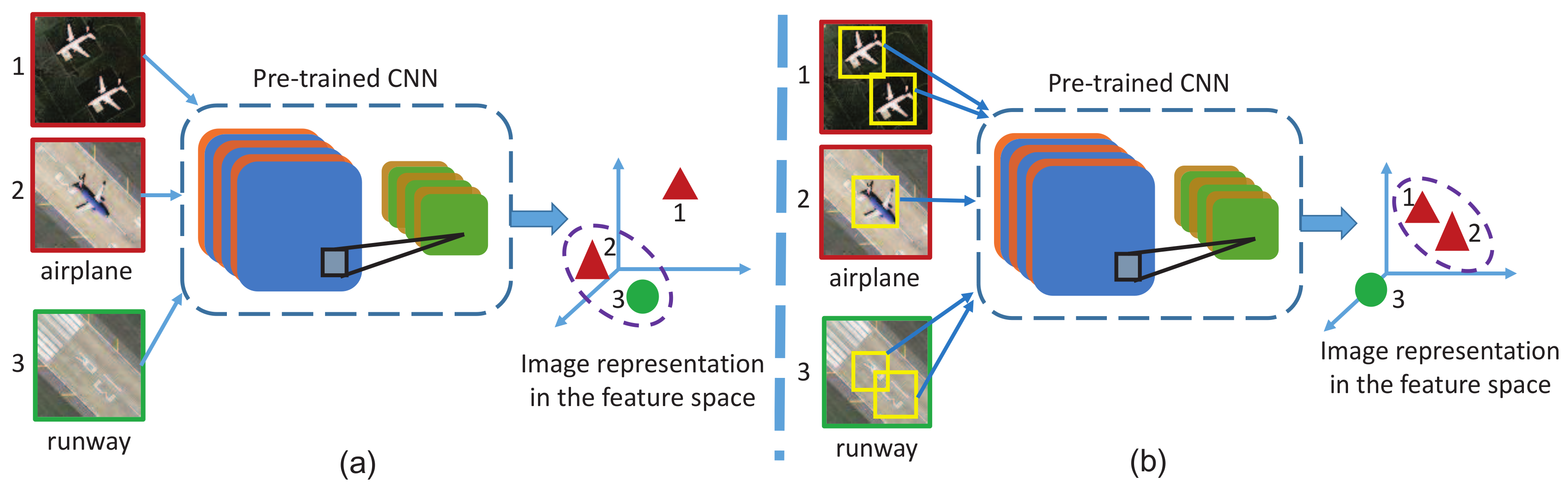
1. Introduction
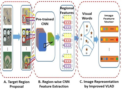
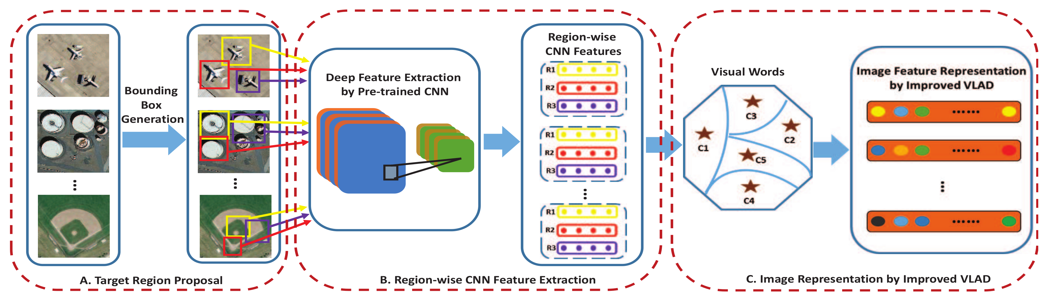
2. The Proposed Approach
2.1. Target Region Proposal
2.2. Region-Wise CNN Feature Extraction
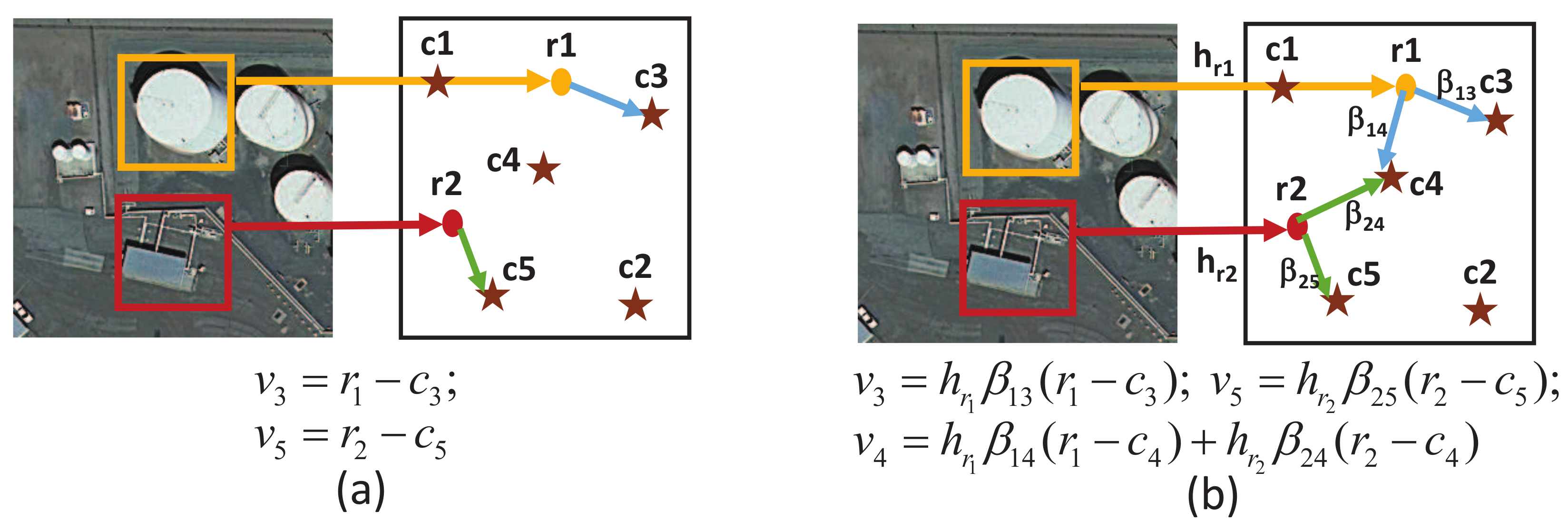
2.3. Image Representation by Improved VLAD
3. Experiments
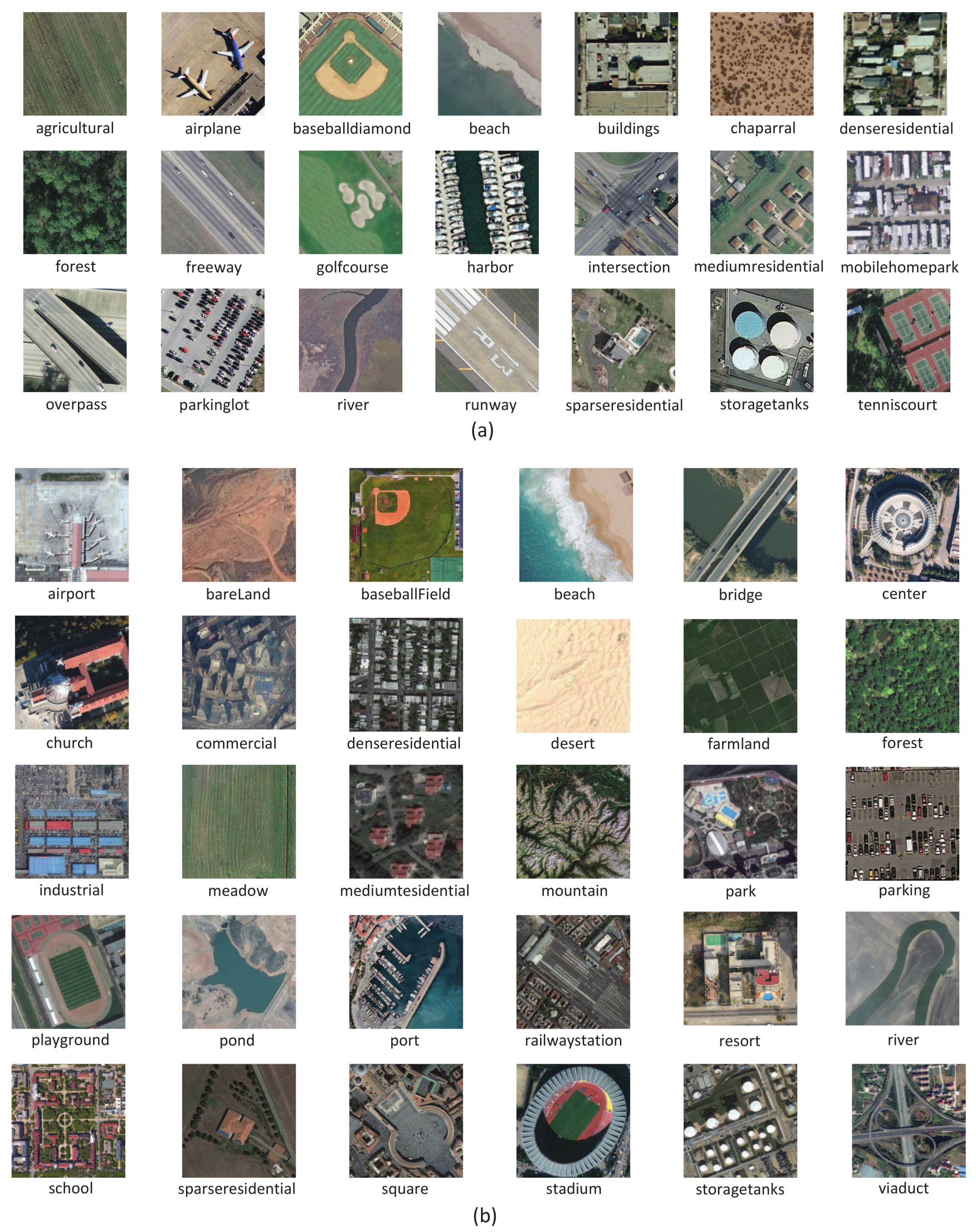
3.1. Datasets and Settings
3.2. Results and Discussion
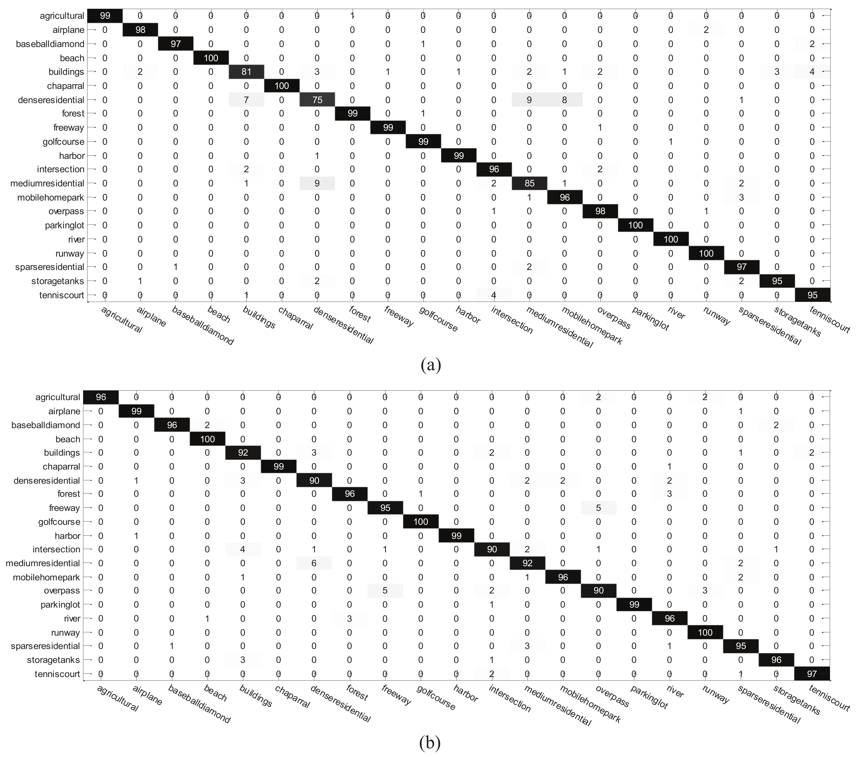
3.2.1. Results for Remote Sensing Scene Classification
3.2.2. Results for Large-Scale Remote Sensing Image Retrieval
4. Future Work
5. Conclusions
Author Contributions
Acknowledgments
Conflicts of Interest
References
- Du, R.; Chen, Y.; Tang, H.; Fang, T. Study on content-based remote sensing image retrieval. In Proceedings of the IEEE International Geoscience and Remote Sensing Symposium (IGARSS), Seoul, Korea, 25–29 July 2005; pp. 707–710. [Google Scholar] [CrossRef]
- Vaduva, C.; Gavat, I.; Datcu, M. Latent dirichlet allocation for spatial analysis of satellite images. IEEE Trans. Geosci. Remote Sens. 2013, 51, 2770–2786. [Google Scholar] [CrossRef]
- Rosu, R.; Donias, M.; Bombrun, L.; Said, S.; Regniers, O.; Da Costa, J.-P. Structure tensor Riemannian statistical models for CBIR and classification of remote sensing images. IEEE Trans. Geosci. Remote Sens. 2017, 55, 248–260. [Google Scholar] [CrossRef]
- Cheng, G.; Han, J.; Lu, X. Remote sensing image scene classification: Benchmark and state of the art. Proc. IEEE 2017, 105, 1865–1883. [Google Scholar] [CrossRef]
- Ozkan, S.; Ates, T.; Tola, E.; Soysal, M.; Esen, E. Performance analysis of state-of-the-art representation methods for geographical image retrieval and categorization. IEEE Geosci. Remote Sens. Lett. 2014, 11, 1996–2000. [Google Scholar] [CrossRef]
- Yang, J.; Liu, J.; Dai, Q. An improved Bag-of-Words framework for remote sensing image retrieval in large-scale image databases. Int. J. Digit. Earth 2015, 8, 273–292. [Google Scholar] [CrossRef]
- Dos Santos, J.; Penatti, O.; Da Silva Torres, R. Evaluating the potential of texture and color descriptors for remote sensing image retrieval and classification. In Proceedings of the Fifth International Conference on Computer Vision Theory and Applications (VISAPP), Angers, France, 17–21 May 2010; pp. 203–208. [Google Scholar]
- Romero, A.; Gatta, C.; Camps-Valls, G. Unsupervised deep feature extraction for remote sensing image classification. IEEE Trans. Geosci. Remote Sens. 2016, 54, 1349–1362. [Google Scholar] [CrossRef]
- Wang, Q.; Wan, J.; Yuan, Y. Locality constraint distance metric learning for traffic congestion detection. Pattern Recogn. 2018, 75, 272–281. [Google Scholar] [CrossRef]
- Aptoula, E. Remote sensing image retrieval with global morphological texture descriptors. IEEE Trans. Geosci. Remote Sens. 2014, 52, 3023–3034. [Google Scholar] [CrossRef]
- Newsam, S.; Wang, L.; Bhagavathy, S.; Manjunath, B.S. Using texture to analyze and manage large collections of remote sensed image and video data. Appl. Opt. 2004, 43, 210–217. [Google Scholar] [CrossRef] [PubMed]
- Luo, B.; Aujol, J.F.; Gousseau, Y.; Ladjal, S. Indexing of satellite images with different resolutions by wavelet features. IEEE Trans. Image Process. 2008, 17, 1465–1472. [Google Scholar] [CrossRef] [PubMed]
- Yang, Y.; Newsam, S. Geographic image retrieval using local invariant features. IEEE Trans. Geosci. Remote Sens. 2013, 51, 818–832. [Google Scholar] [CrossRef]
- Du, Z.; Li, X.; Lu, X. Local structure learning in high resolution remote sensing image retrieval. Neurocomputing 2016, 207, 813–822. [Google Scholar] [CrossRef]
- Lazebnik, S.; Schmid, C.; Ponce, J. Beyond bags of features: Spatial pyramid matching for recognizing natural scene categories. In Proceedings of the IEEE Conference on Computer Vision and Pattern Recognition (CVPR), New York, NY, USA, 17–22 June 2006; pp. 2169–2178. [Google Scholar] [CrossRef]
- Yang, Y.; Newsam, S. Bag-of-visual-words and spatial extensions for land-use classification. In Proceedings of the ACM SIGSPATIAL International Symposium on Advances in Geographic Information Systems (GIS), San Jose, CA, USA, 3–5 November 2010; pp. 270–279. [Google Scholar] [CrossRef]
- Yang, Y.; Newsam, S. Spatial pyramid co-occurrence for image classification. In Proceedings of the IEEE International Conference on Computer Vision (ICCV), Barcelona, Spain, 6–13 November 2011; pp. 1465–1472. [Google Scholar] [CrossRef]
- Cheriyadat, A. Unsupervised feature learning for aerial scene classification. IEEE Trans. Geosci. Remote Sens. 2014, 52, 439–451. [Google Scholar] [CrossRef]
- Zhang, F.; Du, B.; Zhang, L. Saliency-guided unsupervised feature learning for scene classification. IEEE Trans. Geosci. Remote Sens. 2015, 53, 2175–2184. [Google Scholar] [CrossRef]
- Zhou, W.; Shao, Z.; Diao, C.; Cheng, Q. High-resolution remotesensing imagery retrieval using sparse features by auto-encoder. Remote Sens. Lett. 2015, 6, 775–783. [Google Scholar] [CrossRef]
- Li, Y.; Zhang, Y.; Tao, C.; Zhu, H. Content-based high-resolution remote sensing image retrieval via unsupervised feature learning and collaborative affinity metric fusion. Remote Sens. 2016, 8, 709. [Google Scholar] [CrossRef]
- Wang, Y.; Zhang, L.; Tong, X.; Zhang, L.; Zhang, Z.; Liu, H.; Xing, X.; Takis Mathiopoulos, P. A three-layered graph-based learning approach for remote sensing image retrieval. IEEE Trans. Geosci. Remote Sens. 2016, 54, 6020–6034. [Google Scholar] [CrossRef]
- Krizhevsky, A.; Sutskever, I.; Hinton, G. ImageNet classification with deep convolutional neural networks. In Proceedings of the 25th International Conference on Neural Information Processing Systems (NIPS), Lake Tahoe, NV, USA, 3–6 December 2012; pp. 1097–1105. [Google Scholar]
- Simonyan, K.; Zisserman, A. Very deep convolutional networks for large-scale image recognition. In Proceedings of the International Conference on Learning Representations (ICLR), San Diego, CA, USA, 7–9 May 2015; pp. 1–13. [Google Scholar]
- Szegedy, C.; Liu, W.; Jia, Y.; Sermanet, P.; Reed, S.; Anguelov, D.; Erhan, D.; Vanhoucke, V.; Rabinovich, A. Going deeper with convolutions. In Proceedings of the IEEE Conference on Computer Vision and Pattern Recognition (CVPR), Boston, MA, USA, 7–12 June 2015; pp. 1–9. [Google Scholar] [CrossRef]
- Penatti, O.; Nogueira, K.; Dos Santos, J. Do deep features generalize from everyday objects to remote sensing and aerial scenes domains? In Proceedings of the IEEE Conference on Computer Vision and Pattern Recognition Workshops (CVPRW), Boston, MA, USA, 7–12 June 2015; pp. 44–51. [Google Scholar] [CrossRef]
- Wang, Q.; Wan, J.; Yuan, Y. Deep metric learning for crowdedness regression. IEEE Trans. Circ. Syst. Video 2017. [Google Scholar] [CrossRef]
- Wang, Q.; Gao, J.; Yuan, Y. A joint convolutional neural networks and context transfer for street scenes labeling. IEEE Trans. Intell. Transp. 2018, 19, 1457–1470. [Google Scholar] [CrossRef]
- Dutta, R.; Aryal, J.; Das, A.; Kirkpatrick, J.B. Deep cognitive imaging systems enable estimation of continental-scale fire incidence from climate data. Sci. Rep. 2013, 3, 3188. [Google Scholar] [CrossRef] [PubMed]
- Dutta, R.; Das, A.; Aryal, J. Big data integration shows Australian bush-fire frequency is increasing significantly. R. Soc. Open Sci. 2016, 3, 150241. [Google Scholar] [CrossRef] [PubMed]
- Zhang, F.; Du, B.; Zhang, L. Scene classification via a gradient boosting random convolutional network framework. IEEE Trans. Geosci. Remote Sens. 2016, 54, 1793–1802. [Google Scholar] [CrossRef]
- Hu, F.; Xia, G.; Hu, J.; Zhang, L. Transferring deep convolutional neural networks for the scene classification of high-resolution remote sensing imagery. Remote Sens. 2015, 7, 14680–14707. [Google Scholar] [CrossRef]
- Zou, Q.; Ni, L.; Zhang, T.; Wang, Q. Deep learning based feature selection for remote sensing scene classification. IEEE Geosci. Remote Sens. Lett. 2015, 12, 2321–2325. [Google Scholar] [CrossRef]
- Zhou, W.; Newsam, S.; Li, C.; Shao, Z. Learning low dimensional convolutional neural networks for high-resolution remote sensing image retrieval. Remote Sens. 2017, 9, 489. [Google Scholar] [CrossRef]
- Lin, D.; Fu, K.; Wang, Y.; Xu, G.; Sun, X. MARTA GANs: Unsupervised representation learning for remote sensing image classification. IEEE Geosci. Remote Sens. Lett. 2017, 14, 2092–2096. [Google Scholar] [CrossRef]
- Yu, Y.; Gong, Z.; Wang, C.; Zhong, P. An unsupervised convolutional feature fusion network for deep representation of remote sensing images. IEEE Geosci. Remote Sens. Lett. 2018, 15, 23–27. [Google Scholar] [CrossRef]
- Lu, X.; Zheng, X.; Yuan, Y. Remote sensing scene classification by unsupervised representation learning. IEEE Trans. Geosci. Remote Sens. 2017, 55, 5148–5157. [Google Scholar] [CrossRef]
- Cheng, G.; Li, Z.; Yao, X.; Guo, L.; Wei, Z. Remote sensing image scene classification using bag of convolutional features. IEEE Geosci. Remote Sens. Lett. 2017, 14, 1735–1739. [Google Scholar] [CrossRef]
- Li, Y.; Zhang, Y.; Huang, X.; Zhu, H.; Ma, J. Large-scale remote sensing image retrieval by deep hashing neural networks. IEEE Trans. Geosci. Remote Sens. 2018, 56, 950–965. [Google Scholar] [CrossRef]
- Zitnick, C.; Dollár, P. Edge boxes: Locating object proposals from edges. In Proceedings of the 13th European Conference on Computer Vision, Zurich, Switzerland, 6–12 September 2014; pp. 391–405. [Google Scholar] [CrossRef]
- Jégou, H.; Perronnin, F.; Douze, M.; Sanchez, J.; Perez, P.; Schmid, C. Aggregating local image descriptors into compact codes. IEEE Trans. Pattern Anal. Mach. Intell. 2012, 34, 1704–1716. [Google Scholar] [CrossRef]
- Xia, G.; Hu, J.; Hu, F.; Shi, B.; Bai, X.; Zhong, Y.; Zhang, L.; Lu, X. AID: A benchmark dataset for performance evaluation of aerial scene classification. IEEE Trans. Geosci. Remote Sens. 2017, 55, 3965–3981. [Google Scholar] [CrossRef]
- Ye, S.; Pontius, R.G.; Rakshit, R. A review of accuracy assessment for object-based image analysis: From per-pixel to per-polygon approaches. ISPRS J. Photogramm. 2018, 141, 137–147. [Google Scholar] [CrossRef]
- Stein, A.; Aryal, J.; Gort, G. Use of the Bradley-Terry model to quantify association in remotely sensed images. IEEE Trans. Geosci. Remote Sens. 2005, 43, 852–856. [Google Scholar] [CrossRef]
- Demir, B.; Bruzzone, L. Hashing-based scalable remote sensing image search and retrieval in large archives. IEEE Trans. Geosci. Remote Sens. 2016, 54, 892–904. [Google Scholar] [CrossRef]
- Li, P.; Ren, P. Partial randomness hashing for large-scale remote sensing image retrieval. IEEE Geosci. Remote Sens. Lett. 2017, 14, 464–468. [Google Scholar] [CrossRef]
- Ye, D.; Li, Y.; Tao, C.; Xie, X.; Wang, X. Multiple feature hashing learning for large-scale remote sensing image retrieval. ISPRS Int. J. Geo-Inf. 2017, 6, 364. [Google Scholar] [CrossRef]
- Liu, W.; Wang, J.; Ji, R.; Jiang, Y.; Chang, S. Supervised hashing with kernels. In Proceedings of the IEEE Conference on Computer Vision and Pattern Recognition (CVPR), Providence, RI, USA, 16–21 June 2012; pp. 2074–2081. [Google Scholar] [CrossRef]
- Shen, F.; Shen, C.; Liu, W.; Shen, H. Supervised discrete hashing. In Proceedings of the IEEE Conference on Computer Vision and Pattern Recognition (CVPR), Boston, MA, USA, 7–12 June 2015; pp. 37–45. [Google Scholar] [CrossRef]
- Kang, W.; Li, W.; Zhou, Z. Column sampling based discrete supervised hashing. In Proceedings of the Thirtieth AAAI Conference on Artificial Intelligence (AAAI), Phoenix, AZ, USA, 12–17 February 2016; pp. 1230–1236. [Google Scholar]


| Method | Year | Accuracy |
|---|---|---|
| SPMK [15] | 2006 | 74% |
| LDA-SVM [2] | 2013 | 80.33% |
| SIFT + SC [18] | 2014 | 81.67% |
| Saliency + SC [19] | 2015 | 82.72% |
| DCGANs [35] (without augmentation) | 2017 | 85.36% |
| MAGANs [35] (without augmentation) | 2017 | 87.69% |
| CaffeNet [26] (without fine-tuning) | 2015 | 93.42% |
| CaffeNet + VLAD [32] | 2015 | 95.39% |
| UCFFN [36] | 2018 | 87.83% |
| WDM [37] | 2017 | 95.71% |
| CNN-W (AlexNet) with SVM | 95.61% | |
| CNN-R (AlexNet) with SVM | 95.85% | |
| Method | 8-Bits | 12-Bits | 16-Bits | 24-Bits |
|---|---|---|---|---|
| KSH + CNN-W | 0.35 | 0.45 | 0.48 | 0.55 |
| SDH + CNN-W | 0.52 | 0.63 | 0.67 | 0.46 |
| COSDISH + CNN-W | 0.65 | 0.75 | 0.82 | 0.86 |
| KSH + CNN-R | 0.42 | 0.46 | 0.54 | 0.59 |
| SDH + CNN-R | 0.54 | 0.62 | 0.67 | 0.64 |
| COSDISH + CNN-R | 0.74 | 0.86 | 0.88 | 0.91 |
© 2018 by the authors. Licensee MDPI, Basel, Switzerland. This article is an open access article distributed under the terms and conditions of the Creative Commons Attribution (CC BY) license (http://creativecommons.org/licenses/by/4.0/).
Share and Cite
Li, P.; Ren, P.; Zhang, X.; Wang, Q.; Zhu, X.; Wang, L. Region-Wise Deep Feature Representation for Remote Sensing Images. Remote Sens. 2018, 10, 871. https://doi.org/10.3390/rs10060871
Li P, Ren P, Zhang X, Wang Q, Zhu X, Wang L. Region-Wise Deep Feature Representation for Remote Sensing Images. Remote Sensing. 2018; 10(6):871. https://doi.org/10.3390/rs10060871
Chicago/Turabian StyleLi, Peng, Peng Ren, Xiaoyu Zhang, Qian Wang, Xiaobin Zhu, and Lei Wang. 2018. "Region-Wise Deep Feature Representation for Remote Sensing Images" Remote Sensing 10, no. 6: 871. https://doi.org/10.3390/rs10060871
APA StyleLi, P., Ren, P., Zhang, X., Wang, Q., Zhu, X., & Wang, L. (2018). Region-Wise Deep Feature Representation for Remote Sensing Images. Remote Sensing, 10(6), 871. https://doi.org/10.3390/rs10060871