Detection of Spatiotemporal Extreme Changes in Atmospheric CO₂ Concentration Based on Satellite Observations

Abstract

Atmospheric CO₂ concentrations are sensitive to the effects of climate extremes on carbon sources and sinks of the land biosphere. Therefore, extreme changes of atmospheric CO₂ can be used to identify anomalous sources and sinks of carbon. In this study, we develop a spatiotemporal extreme change detection method for atmospheric CO₂ concentrations using column-averaged CO₂ dry air mole fraction (XCO₂) retrieved from the Greenhouse gases Observing SATellite (GOSAT) from 1 June 2009 to 31 May 2016. For extreme events identified, we attributed the main drivers using surface environmental parameters, including surface skin temperature, self-calibrating Palmer drought severity index, burned area, and gross primary production (GPP). We also tested the sensitivity of XCO₂ response to changing surface CO₂ fluxes using model simulations and Goddard Earth Observing System (GEOS)-Chem atmospheric transport. Several extreme high XCO₂ events are detected around mid-2010 over Eurasia and in early 2016 in the tropics. The magnitudes of extreme XCO₂ increases are around 1.5–1.8 ppm in the Northern Hemisphere and 1.2–1.4 ppm in Southern Hemisphere. The spatiotemporal pattern of detected high XCO₂ events are similar to patterns of local surface environmental parameter extremes. The extreme high XCO₂ events often occurred during periods of increased temperature, severe drought, increased wildfire or reduced GPP. Our sensitivity tests show that the magnitude of detectable anomalies varies with location, for example 25% or larger anomalies in local CO₂ emission fluxes are detectable in tropical forest, whereas anomalies must be half again as large in mid-latitudes (~37.5%). In conclusion, we present a method for extreme high XCO₂ detection, and large changes in land CO₂ fluxes. This provides another tool to monitor large-scale changes in the land carbon sink and potential feedbacks on the climate system.

1. Introduction

The global mean atmospheric CO₂ concentration is increasing on average at a rate of 2.38 ppm yr⁻¹ in recent years, due to anthropogenic CO₂ emissions in excess of carbon uptake by land and ocean sinks [1]. The annual increase is quite variable, for example the standard deviation from 2009 to 2016 was 0.44 ppm yr⁻¹ [2]. Carbon sources/sinks from the terrestrial biosphere contribute most to the inter-annual variability [3]. Climate extremes like drought and heat waves have been shown to result in large changes in carbon sources and sinks of terrestrial biosphere, which have the potential to substantially modify regional carbon dioxide (CO₂) uptake/release [4]. As a result, regional atmospheric CO₂ concentration could vary with climate change in addition to the global atmospheric CO₂ growth rate. The change of atmospheric CO₂ concentration is not only impacted by anomalous terrestrial biosphere CO₂ uptake or release, caused by anomalous weather events, but also intensifying climate changes [5,6]. Understanding the relationship between the CO₂ concentration changes response to climate events, makes an important contribution to carbon sources and sinks change detection and forecasting [7].

Extreme weather events have increased and are predicted to increase in the frequency as result of global warming [6,8,9,10,11]. They attract social interest for their fundamental impacts on the natural environment and human society [12,13]. Previous research has attempted to link extreme events and their effects on the land carbon sink. Combining reanalysis data and remote sensing observations, Schwalm et al. [4] found that the drought during 2000–2004 in western North America reduced carbon uptake by 30–298 TgC/yr. During the heat and drought in 2003 over Europe, the gross primary production (GPP) was decreased by 30%, which resulted in strong anomalous CO₂ emission of 0.5 PgC/yr [14]. From the extreme wildfires in western Russia over the summer of 2010, CO₂ emission increased 255.76 Tg based on satellite data [15]. The drought over that period can be also captured by satellite observed solar-induced chlorophyll fluorescence (SIF) [16]. Anomalous carbon uptake over Australia around 2011 was also discovered with satellite observations and model simulations [17]. Extreme drought events in North America during 2011 and 2012 were also selected as a case, for checking the capability of using SIF to characterize vegetation response to climate change [18]. The strong 2015/2016 El Niño [19,20,21] may have increased carbon flux releases by 0.9 ± 0.29, 0.8 ± 0.22, and 0.8 ± 0.28 GtC over the tropical continents including South America, Africa and Asia [22]. These studies show how carbon fluxes anomalies associated with extreme climate events can impact atmospheric CO₂ concentrations.

There is also great potential in identifying anomalous changes in the land carbon sink without prior knowledge of extreme weather events [23,24,25]. Variations in atmospheric CO₂ can be used for anomalous carbon source and sink change analysis. The column-averaged CO₂ dry air mole fraction (XCO₂) derived from the Greenhouse gases Observing SATellite (GOSAT) proved valuable for confirming the effect of extreme climate events (such as El Niño) on the CO₂ concentration [26]. However, the gaps in time and space limit the satellite retrieved XCO₂ from probing the time and space of carbon sources and sinks anomalies.

In this study, we use XCO₂ time series from satellite observations with global mapping [27,28] for extreme high XCO₂ detection. In contrast to earlier studies, which concentrated on surface environment variables (such as fraction of absorbed photosynthetically active radiation (fPAR), GPP, surface temperature and so on) [29,30,31], we focus on using atmospheric CO₂ concentration for extreme event detection. CO₂ anomalies integrate influences from many biosphere–atmospheric interaction, including carbon uptake/release from soil ecological activity, vegetation activity, biomass burning, etc. In addition, XCO₂ anomalies can be connected across time and space as a result of atmospheric transport. We aim to develop an approach for detecting spatiotemporal continuum high XCO₂ anomalies using satellite XCO₂ observations, which are related to terrestrial biosphere anomalies of CO₂ uptake and release. The detected high XCO₂ can be attributed to carbon source/sink changes caused by extreme weather events. The dataset used in this study and its preprocess is described in Section 2. The method of extreme events detection can be found in Section 3. Corresponding results of the extreme detection are revealed in Section 4. Discussion of the detected spatial pattern over specific duration and correlation between XCO₂ and local CO₂ flux is in Section 5, and conclusions are presented in Section 6.

2. Datasets and Pre-Processing Steps

The datasets used in this analysis are summarized in

Table 1. Summary of the datasets used in this study. XCO₂ from global mapping of satellite observations (GM-XCO₂) and model simulation (CarbonTracker: CT-XCO₂ and GEOS-Chem (described in Section 2.2): GEOS-XCO₂), biospheric CO₂ fluxes from SiB3 used in GEOS-Chem, environmental parameters including surface skin temperature (Temp), self-calibrating Palmer drought severity index (scPDSI), burned area (BA), and gross primary production (GPP). The spatial and temporal resolution of the observations or model products are indicated as well as a reference describing the products in more detail.

Data	Source	Space Res.	Time Res.	Reference
GM-XCO2	Mapping data from ACOS GOSAT v7.3	1.0 × 1.0 de.	3 days	O’Dell et al. [33] Zeng et al. [28]
CT-XCO2	CarbonTracker 2016	2.0 × 3.0 de.	3 h	Peter et al. [50]
GEOS-XCO2	GEOS-Chem v11.1	2.0 × 2.5 de.	3 h	Nassar et al. [51]
SiB3 CO2 flux	Simple Biosphere Model, version 3	1.0 × 1.25 de	3 h	Sellers et al. [52]
Temp	AIRSX3STM v6.0, produced with AIRS and AMSU	1.0 × 1.0 de.	monthly	Huffman et al. [53]
scPDSI	CRU TS 3.25	0.5 × 0.5 de.	monthly	Wells et al. [54]
BA	GFED v4.0	0.25 × 0.25 de.	monthly	Giglio et al. [55]
GPP	MOD17A2 v5	1.0 × 1.0 km	monthly	Heinsch et al. [56]; Zhao et al. [57]

and include XCO₂ from satellite (GOSAT) and model simulations (CarbonTracker and Goddard Earth Observing System (GEOS)-Chem), biospheric CO₂ fluxes from Simple Biosphere Model, version 3 (SiB3) used in GEOS-Chem, and related surface environmental parameters including surface skin temperature (Temp), self-calibrating Palmer drought severity index (scPDSI), burned area (BA), and GPP. Detailed information about data set versions and their characteristics will be described in the following sections. The spatial and temporal scope of our analysis covers land areas from 45°S to 60°N, from June 2009 to May 2016.

2.1. Mapping XCO₂ from Satellite Observations

GOSAT is the first satellite dedicated for greenhouse gas observations. Developed by the Japan Aerospace Exploration Agency (JAXA), it launched in January 2009 [32]. We collected the column-averaged CO₂ dry air mole fraction (XCO₂) of GOSAT observations, with the retrieval method provided by the Atmospheric CO₂ Observations from Space (ACOS) project team [33] (hereafter referred as ACOS-GOSAT). The ACOS-GOSAT XCO₂ v7.3 retrieval spans from 1 June 2009 to 31 May 2016. Gaps in observations were filled using an interpolation method to create global land maps of XCO₂ (GM-XCO₂), with spatial resolution of 1 × 1 degree and time resolution of 3 days [27,28]. The GM-XCO₂ maps are used for the spatiotemporal extreme event detection based on high XCO₂ anomalies in this study.

Cross-validation based on a Monte Carlo sampling technique was used to assess the accuracy of the GM-XCO₂ product. The result is shown in Figure S1. It shows good agreement between predicted GM-XCO₂ and observed (no interpolation) XCO₂ with a high coefficient of determination (R² = 0.94) and a low mean absolute prediction error (MAPE) of 0.85 ppm. GM-XCO₂ was also compared with observed XCO₂ from ground-based sites from the Total Carbon Column Observing Network (TCCON) [34,35,36,37,38,39,40,41,42,43,44,45,46,47,48,49] as shown in Figure S2. Averaged absolute bias between GM-XCO₂ and TCCON observations are around 1 ppm with a standard deviation of 1.51 ppm, shown in Table S1. Detailed information on the GM-XCO₂ validation method can be found in He et al. [27] and Zeng et al. [28].

2.2. XCO₂ from Model Simulations

We also compared the results from CarbonTracker 2016. CarbonTracker is a model-data assimilation system and annual updates provide atmospheric CO₂ mixing ratio distributions and inferred surface fluxes [50]. CarbonTracker uses the Carnegie–Ames–Stanford Approach (CASA) land surface model to estimate priors and Transport Model 5 (TM5) to represent atmospheric circulation [58]. CarbonTracker version 2016 provide atmospheric CO₂ concentration from 1 January 2009 to 31 December 2015 [59]. We calculated the XCO₂ from the CarbonTracker atmospheric distribution of CO₂ (CT-XCO₂), with spatial resolution of 2 × 3 degrees and time resolution of 3 days, using the CO₂ profile data within the local time around 13:00, with the pressure-averaged method described in Conner et al. [60]. After that, CT-XCO₂ was downscaled to be 1 × 1 degrees using the nearest neighbor.

We tested the sensitivity of XCO₂ to changes in surface fluxes using a collection of surface flux estimates and the GEOS-Chem global chemical transport model (CTM) assimilated with meteorological fields from the National Aeronautics and Space Administration (NASA) Goddard Earth Observing System (GEOS) [51,61]. Surface CO₂ fluxes used in GEOS-Chem include fossil fuel emission from Open-source Data Inventory for Anthropogenic CO₂ (ODIAC); biomass burning from the Global Fire Emission Database (GFED3); ocean exchange from Takahashi et al. [62] and annual biofuel fluxes from Yevich and Logan [63]. Biospheric CO₂ fluxes used for this simulation were from the SiB3 [52]. The biospheric fluxes from SiB3 were not available for our entire study period (only 2006 through 2010), therefore, we only use them as a way to test the influence of atmospheric transport on extreme XCO₂ detection. In order to calculate the extreme XCO₂ detection from the GEOS-Chem sensitivity test, we did need to use biospheric flux estimates for the entire record. For this purpose, we used only 2009 flux repeated from 2010 to 2015. This was important for determining the Z score (described in Section 3.2) of the GEOS-Chem simulation. We simulated atmospheric CO₂ concentration from 1 January 2009 to 31 December 2015, using GEOS-Chem, version 11.1. The model used here is driven by 3 hourly assimilated meteorological observations from GEOS at 2° (latitude) by 2.5° (longitude) horizontal resolution with 47 vertical layers. The GEOS-Chem XCO₂ (GEOS-XCO₂) was calculated with the average kernel [60] of GOSAT XCO₂ within the local time around 13:00. After that, GEOS-XCO₂ was resampled to be 1 × 1 degrees similar as that of CT-XCO₂. We emphasize that this model simulation is not intended to match observations.

2.3. Surface Environmental Parameters Related to CO₂ Uptake and Release

Surface parameters that we explored included land surface skin temperature (temp), scPDSI, BA, and GPP. We obtained the temperature data from NASA [64], which uses a standard physical retrieval that is combination of data from the Atmospheric Infrared Sounder (AIRS) and the Advanced Microwave Sounding Unit (AMSU) [65]. We used the level 3 monthly product with spatial resolution of 1 × 1 degrees from January 2009 to September 2016 for AMSU limitation later. The drought severity index, scPDSI, used for quantifying long-term drought conditions, are calculated with time series of temperature, together with fixed parameters related to the soil/surface characteristics at each location, which aims to make results from different climate regimes more comparable [54]. This index was available as monthly 0.5 degree from January 2009 to December 2016. Monthly BA, from Global Fire Emissions Database, Version 4.0 (GFED4), had a spatial resolution of 0.25 degree from January 2009 to December 2016. The product combined Moderate Resolution Imaging Spectroradiometer (MODIS) burned area maps with active fire data from the Tropical Rainfall Measuring Mission (TRMM) Visible and Infrared Scanner (VIRS) and the Along-Track Scanning Radiometer (ATSR) family of sensors [55]. GPP, a parameter related to carbon uptake by vegetation photosynthesis, was obtained from MODIS. Monthly GPP was produced with the data of time resolution of 8 days [56,57]. GPP with spatial resolution of 1 km data from 2009 to 2015 was collected from [66], and data of 2016 are calculated with data accumulation directly. In addition, The Land Cover Type Climate Modeling Grid (CMG) product (MCD12C1) from MODIS [67] in 2009 was used for land cover classification over detected results.

Quality control was performed on all datasets according to their respective user guides and resampled to 1 × 1° degree spatial resolution to match GM-XCO₂ using grid averaging. A mean seasonal cycle was calculated for each time series similar to GM-XCO₂ in order to identify anomalies in time and space.

3. Methods

3.1. Extreme XCO₂ Change and Data Preprocess

To quantify XCO₂ anomalies in satellite observations and model simulations, we need to remove the XCO₂ background increase due to fossil fuel emissions and the mean seasonal cycle. The fitting method used a combination of a linear function and annual periodic function as shown in Equation (1),

$$\mathrm{x}\left(\mathrm{t}\right)={\mathrm{k}}_0+{\mathrm{k}}_1\mathrm{t}+{{\displaystyle \sum }}_{\mathrm{i}=1}^2({\mathrm{a}}_{\mathrm{i}}\cos \left(2\mathsf{\pi }\mathrm{it}\right)+{\mathrm{b}}_{\mathrm{i}}\sin \left(2\mathsf{\pi }\mathrm{it}\right))+\mathsf{\delta }.$$

(1)

where x(t) represents the XCO₂ in time t. ${\mathrm{k}}_0$ represents the mean XCO₂ at the start of the time series, ${\mathrm{k}}_1\mathrm{t}$ represents the XCO₂ gradual trend mainly caused by anthropogenic CO₂ emissions [1], which is assumed to be a linear increase. The term ${{\displaystyle \sum }}_{\mathrm{i}=1}^2({\mathrm{a}}_{\mathrm{i}}\cos \left(2\mathsf{\pi }\mathrm{it}\right)+{\mathrm{b}}_{\mathrm{i}}\sin \left(2\mathsf{\pi }\mathrm{it}\right))$ characterizes the XCO₂ seasonal cycle, driven by CO₂ biosphere–atmosphere interactions [68,69,70]; and $\mathsf{\delta }$ is the fitting residual, which consist of random error and extreme anomalies in surface carbon uptake/release. Parameter values in Equation (1) are optimized to reduce the residuals between least square fitting using Equation (1) and the GM-XCO₂ observations. An example fitting in one grid can be seen in He et al. [27].

3.2. Spatial-Temporal Extreme High XCO₂ Detection

We define extreme high XCO₂ as the spatiotemporal continuum units whose fitting residuals deviate outside of the normal range of high probability values [7,30]. For each grid, we calculate a Z score of fitting residuals to standardize across differences in the magnitude of residuals according to Equation (2). The Z score, $\mathrm{Z}\left(\mathrm{i},\mathrm{j},\mathrm{t}\right)$, is calculated from the XCO₂ fitting residuals, $\mathsf{\delta }$ but also described as dXCO₂ throughout the manuscript, in a grid with latitude i, longitude j, and time t, and $\mathrm{mean}\left(\mathsf{\delta }\left(\mathrm{i},\mathrm{j}\right)\right)$ and $\mathrm{std}\left(\mathsf{\delta }\left(\mathrm{i},\mathrm{j}\right)\right)$ represent the mean and standard deviation value of the time series in location (i, j).

$$\mathrm{Z}\left(\mathrm{i},\mathrm{j},\mathrm{t}\right)=\left(\mathsf{\delta }\left(\mathrm{i},\mathrm{j},\mathrm{t}\right)-\mathrm{mean}\left(\mathsf{\delta }\left(\mathrm{i},\mathrm{j}\right)\right)\right)/\mathrm{std}\left(\mathsf{\delta }\left(\mathrm{i},\mathrm{j}\right)\right),$$

(2)

We selected the Gaussian model, a simple spatiotemporal outlier detection technique to define anomalously high XCO₂ in Equation (3a). This test identifies grids where dXCO₂ (or δ) is much larger than a threshold, ${\mathsf{\mu }}_1$, and has a Z score of the dXCO₂ variability that exceeds a threshold, ${\mathsf{\mu }}_2.$ In this study, ${\mathsf{\mu }}_1$ is set to be 1.0, according to a priori knowledge of XCO₂ concentration’s precision from GOSAT retrievals, and ${\mathsf{\mu }}_2$ is set to 1.96, which represents the 95% threshold in the Gaussian distribution. The logic test is described using ‘$\mathrm{bool}$’; true = 1 and false = 0. The connectivity of the extreme units are tested as well. $\mathrm{D}\left(\Delta \mathrm{i},\Delta \mathrm{j},\Delta \mathrm{t}\right)$ represents the spatiotemporal distance between grids (Equation (4)). The distance threshold is d and the connectivity threshold is n. Thresholds d and n were set to be 1 (minimum distance) and 3 (mid-value of range from 0 to 6), respectively. In order for an event to count as an extreme event, Equations (3a)–(3c) must all be true.

$$\mathrm{bool}\left(\mathsf{\delta }\left({\mathrm{i}}_0,{\mathrm{j}}_0,{\mathrm{t}}_0\right)>{\mathsf{\mu }}_1\right)\times \mathrm{bool}\left(\mathrm{Z}\left({\mathrm{i}}_0,{\mathrm{j}}_0,{\mathrm{t}}_0\right)>{\mathsf{\mu }}_2\right)=1,$$

(3a)

$${{\displaystyle \sum }}_{\mathrm{i}={\mathrm{i}}_0-\mathrm{d}}^{\mathrm{i}={\mathrm{i}}_0+\mathrm{d}}{{\displaystyle \sum }}_{\mathrm{j}={\mathrm{j}}_0-\mathrm{d}}^{\mathrm{j}={\mathrm{j}}_0+\mathrm{d}}{{\displaystyle \sum }}_{\mathrm{t}={\mathrm{t}}_0-\mathrm{d}}^{\mathrm{t}={\mathrm{t}}_0+\mathrm{d}}\{\mathrm{bool}\left(\mathsf{\delta }\left(\mathrm{i},\mathrm{j},\mathrm{t}\right)>{\mathsf{\mu }}_1\right)\times \mathrm{bool}\left(\mathrm{Z}\left(\mathrm{i},\mathrm{j},\mathrm{t}\right)>{\mathsf{\mu }}_2\right)>\mathrm{n}\},$$

(3b)

$$\mathrm{Where}\mathrm{D}\left(\mathrm{i}-{\mathrm{i}}_0,\mathrm{j}-{\mathrm{j}}_0,\mathrm{t}-{\mathrm{t}}_0\right)<\mathrm{d},$$

(3c)

$$\mathrm{D}\left(\Delta \mathrm{i},\Delta \mathrm{j},\Delta \mathrm{t}\right)=\sqrt{{\left(\Delta \mathrm{i}\right)}^2+{\left(\Delta \mathrm{j}\right)}^2+{\left(\Delta \mathrm{t}\right)}^2},$$

(4)

In addition, three-dimensional extreme dXCO₂ can be inspected with the steps above. We defined the extreme XCO₂ events as the space-time continuous unit, e.g., if one grid is selected as extreme high dXCO₂, there are six directions for expansion. If any grid, within the six directions, is also an extreme high dXCO₂, they are included in the same unit. They can further expand in time as well, until no other grid are connected to the unit and we count the total number of grid units to determine the magnitude of the extreme event. Identified units of the space-time continuous grids are then the extreme high XCO₂ units. This procedure is the flood-fill algorithm described in Zscheischler et al. [30]. We used the function of bwconncomp from Matlab to execute the algorithm described above. The work flow of the extreme events detection method is summarized in Figure 1.

3.3. Sensitivity Test of XCO₂ to Changes in Surface CO₂ Fluxes

We investigated the sensitivity of the XCO₂ response to various local CO₂ flux change as a result of atmospheric transport which tend to smooth out anomalous CO₂ concentration. We used GEOS-Chem v11.1 and surface fluxes described in Section 2 to calculated predicted XCO₂ responses. The predicted XCO₂ output was compared to its normal value, described in Section 3.1, to get the changes in XCO₂ (dXCO₂). The method of extreme XCO₂ detection shown in Section 3.2 was applied to discuss whether the predicted dXCO₂ was detectable. We repeated 2009 SiB3 biospheric fluxes and tested enhancements of 25%, 37.5%, 50%, 62.5%, and 75% over the 2009 predictions from July to September of 2009 in six unique regions (as shown in Figure S3): including Eurasia (35°–75°E, 45°–61°N); North America (65°–105°W, 40°–55°N,); South Asia (65°–106°E, 13°–28°N); South America (35°–75°W, 3°–18°S); South Africa (10°–40°E, 10°–30°S) and Australia (120°–150°E, 15°–35°S). The resulting dXCO2 values are calculated from each of these model simulations

4. Results

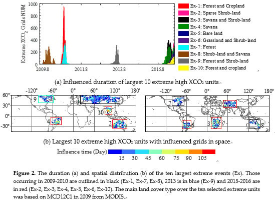
4.1. Extracted Spatiotemporal Continuum Extreme High XCO₂

Here, we show the 10 largest extreme high XCO₂ units (referred to as ‘Ex-1’ through ‘Ex-10’) in Figure 2. The selected high XCO₂ units have grid sums numbering more than 2000 in time and space, and they are identified by their rank number. The spatial distribution of these 10 largest units is separately shown in Figure 2b. There are three (Ex-1, Ex-7, Ex-8), one (Ex-9) and six units (Ex-2, Ex-3, Ex-4, Ex-5, Ex-6, Ex-10) that occurred over the period of 2009–2010, 2013, and 2015–2016, respectively, as shown in Figure 2a. The largest event, Ex-1, occurred in Eurasia, with mixed land cover of forest, cropland and other vegetation, spread from July to October in 2010. It has a large special extent but is relatively concentrated in time. That is consistent with the influence of high temperatures and wildfire in the region [15]. The Ex-7 was distributed over north-eastern North America covered mostly in forest, occurred in the similar period of Ex-1. Ex-8 happened over eastern Australia shrub-land in late of 2009. Ex-9 distributed in the similar space of Ex-7, but happened in mid-2013. The five units (Ex-2, Ex-3, Ex-4, Ex-6, and Ex-10) happened in the tropical continents (Australia sparse shrub-land, southern Africa savanna and shrub-land, eastern and southern South America savanna, grassland and shrub-land, south-eastern Asia forest and cropland, respectively). They occurred from January to May of 2016, although with different duration within that window. These events correspond to the large CO₂ release related to the 2015–2016 EI Niño [22]. Ex-5 occurred over Central Asia bare land in early 2016. In addition, some units (Ex-2 and Ex-8, or Ex-7 and Ex-9) are overlapped in space.

Time series of mean dXCO₂ and XCO₂ over each detected unit are shown in Figure 3. Extremes could happen in more than one area during one time period, and more than one time period in one area. Mean dXCO₂ and corresponding Z scores within detected units both in time and space are summarized in

Table 2. Time and space features of detected extreme units (Ex) 1 through 10. Their land over types, period, grids number (NUM), location, dXCO₂, Z score, and difference between monthly data and its normal value over significant different period about surface skin temperature (ΔTemp), self-calibrating Palmer drought severity index (scPDSI) (negative for drought and vice versa), burned area (ΔBA) and gross primary production (ΔGPP) during the main detected period over these units. Positive values indicate increasing values during the extreme event. Bold items indicate likely contribution to the atmospheric XCO₂ increase, because they represent forcing that likely increases CO₂ flux to the atmosphere.

	Period	Grids NUM (Location)	dXCO2 (ppm)	Z Score	ΔTemp (K)	scPDSI	ΔBA (km2/grid)	ΔGPP (gC/m2)
Ex-1: Forest and Cropland	10 July~10 October	11361 (35–60°N; 21–134°E)	1.77 ± 0.39	2.43 ± 0.39	1.22 ± 1.60	−1.11 ± 0.18	8.77 ± 7.82	−5.85 ± 4.94
Ex-2: Sparse Shrub-land	16 January~16 April	6527 (11–35°S; 113–153°E)	1.28 ± 0.21	2.31 ± 0.30	1.88 ± 0.70	−1.68 ± 0.14	−12.1 ± 20.39	−5.99 ± 3.32
Ex-3: Savanna and Shrub-land	1 February~16 May	5443 (5–35°S; 12–38°E)	1.37 ± 0.27	2.38 ± 0.36	1.93 ± 0.96	−2.10 ± 0.02	1.63 ± 2.43	−19.15 ± 13.64
Ex-4: Savanna	15 November~16 May	4023 (5–25°S; 36–63°W)	1.40 ± 0.23	2.32 ± 0.33	1.56 ± 1.84	−1.31 ± 0.46	1.64 ± 2.82	−26.66 ± 18.97
Ex-5: Bare land	16 March~16 May	3485 (26–45°N; 48–84°E)	1.49 ± 0.30	2.37 ± 0.34	0.56 ± 0.86	0.63 ± 0.13	7.32 ± 19.17	−0.37 ± 0.72
Ex-6: Grassland and Shrub-land	16 February~16 May	2887 (17–35°S; 48–72°W)	1.30 ± 0.27	2.48 ± 0.42	0.54 ± 1.84	1.53 ± 0.19	−0.71 ± 0.58	−16.02 ± 6.15
Ex-7: Forest	10 August~10 October	2727 (31–55°N; 68–102°W)	1.68 ± 0.34	2.32 ± 0.27	1.13 ± 1.11	−0.71 ± 0.21	−0.01 ± 0.03	−4.99 ± 9.74
Ex-8: Shrub-land and Savanna	9 September~9 December	2498 (12–35°S; 123–152°E)	1.39 ± 0.25	2.36 ± 0.34	1.78 ± 0.80	−1.98 ± 0.44	57.47 ± 108.69	−11.50 ± 5.31
Ex-9: Forest and Shrub-land	13 April~13 July	2297 (39–60°N; 61–101°W)	1.40 ± 0.25	2.31 ± 0.31	−0.39 ± 0.85	−0.65 ± 0.28	15.35 ± 21.58	−2.57 ± 2.15
Ex-10: Forest and cropland	16 March~16 May	2236 (6–28°N; 93–109°E)	1.61 ± 0.29	2.31 ± 0.29	2.55 ± 1.07	−0.94 ± 0.10	−3.62 ± 25.08	−26.91 ± 20.88

. The mean dXCO₂ within detected grids was approximately 1.4–1.8 ppm over the Northern Hemisphere (NH) and 1.2–1.4 ppm over the Southern Hemisphere (SH). Units over forest and cropland (Ex-1, Ex-7, Ex-10) are larger than 1.6 ppm, and those over savanna and shrub-land (Ex-2, Ex-3, Ex-4, Ex-6, Ex-8) are around 1.28–1.4 ppm. The mean Z score for all the 10 extremes are around 2.3–2.5 (high values indicate a high probability of extreme high XCO₂).

4.2. Attribution of Detected High XCO₂ Units by Surface Extremes

We attribute extreme high XCO₂ units to local reduced carbon uptake and/or increased carbon release, within at least a portion of the region identified. Some potential local drivers, including temperature, drought index, BA and GPP, are used to discuss the possible local extreme climate over detected extreme XCO₂ units. Monthly mean values of parameters and its normal value (calculated with all data in a given month during the study period) over the detected extreme high XCO₂ units from 2009 to 2016 are shown in Figure 4 and Figure 5. The statistics of the driver anomalies during detected extreme periods and its comparison to the overall fluctuation is shown in Table 2.

We find that abnormal increased temperature (1.22 ± 1.60, 1.78 ± 0.80 K), moderate/severe drought (−1.11 ± 0.18, −1.98 ± 0.44), increased wildfire (8.77 ± 7.82, 57.47 ± 108.69 km²/grid), increased CO₂ release, and reduced GPP (−5.85 ± 4.94, −11.50 ± 5.31 gC/m²), emerge together over the time and space of units Ex-1 and Ex-8. All of them could contribute to the abnormal XCO₂. In 2016 in the SH, XCO₂ anomalies in Ex-2, Ex-3 and Ex-4 resulted from a combination of influences of abnormal increased temperature (1.56 to 1.93 K), severe drought (−1.31 to −2.10), reduced GPP (−5.99 to −26.66 gC/m²). XCO₂ anomaly over Ex-6 could be explained by flooding indicated by abnormal scPDSI (−0.72 compared to a mean 1.53) and reduced GPP (−16.02 ± 6.15 gC/m²). The XCO₂ anomaly in Ex-10 could be explained by the increased temperature (2.55 ± 1.07 K) and large GPP reduction (−26.91 ± 20.88 gC/m²). The XCO₂ anomaly in Ex-9 could be explained by increased fire (with increased BA of 15.35 ± 21.58 km²/grid), which is consistent with the wild fire that occurred in eastern Canada during that period discussed in Erni et al. [71]. Detected abnormal XCO₂ over Ex-7 could be influenced by reduced local carbon uptake (with GPP of −4.99 ± 9.74 gC/m²) and nearby high XCO₂ diffusion, transported from Eurasia as discussed in Guelert et al. [26]. However, no significant surface change is found over Ex-5, although the GPP is slightly reduced (−0.37 ± 0.72 gC/m²). Some changes in the bare land or CO₂ transported in from nearby are discussed in Section 5.1.

4.3. Comparing Satellite Observations and Model Simulations

Here we compare the number of extreme high XCO₂ grids identified from GM-XCO₂ and CarbonTracker 2016 with the monthly Southern Ocillation Index (SOI), related to El Niño and La Niña conditions (Figure 6). The largest extreme event in a high XCO₂ grid number of satellite and model simulations are distributed over summer (around August to September) of 2010. The anomalous grid number of GM-XCO₂ increases from 300 around July to 1100 around September, and dropped to lower than 300 in October. A relatively narrow extreme XCO₂ can be found over late spring and early summer of 2013 both in GM-XCO₂ and CarbonTracker. Another extreme XCO₂ period was found in January–May 2016, which is up to 1300 grid number, from GM-XCO₂ satellite observations. Note that CarbonTracker fluxes were available through 2015 and are not comparable to the 2016 events. Moreover, high values of dXCO₂ Z scores, likely to be extreme, were found over NH in mid-2010, SH and low latitude of early 2016 both in original ACOS-GOSAT XCO₂ and GM-XCO₂, shown in Figure S4.

Extreme XCO₂ events in 2009–2010 in the northern hemisphere occurred during a weak El Nino transition to a strong La Niña. The 2013 event was during weak La Niña conditions, and the 2015–2016 events in the southern hemisphere followed strong El Niño conditions. This analysis shows the global pattern of influence of these characteristic climate patterns on extreme CO₂ fluxes.

4.4. Sensitivity Test of XCO₂ Response to Local Biosphere Flux Change with Goddard Earth Observing System (GEOS)-Chem

We designed a sensitivity test for XCO₂ response to local CO₂ flux changes over six regions shown in Figure S3. The extreme detection method was applied for evaluating how much local CO₂ flux change is required to make the increased XCO₂ detectable. Increased XCO₂ are predicted using the GEOS-Chem atmospheric transport model by assuming different carbon flux inputs, described in Section 3.3. CO₂ fluxes with emission increases of 25%, 37.5%, 50%, 62.5% and 75% were added to the model input to create different XCO₂ simulations. The increased XCO₂ (ΔXCO₂) response to different local land biosphere CO₂ flux changes are shown in Figure 7. Increased XCO₂ is linear to the local CO₂ change with atmospheric transport over different regions, but the slope varies by regions. The slopes ranged from 0.32 ppm/ (10⁻⁸ kg/m²/s) in North America to 1.05 ppm/ (10⁻⁸ kg/m²/s) in South Africa. The shallower slopes from South America, North America, Eurasia and South Asia flux anomalies, compared to South Africa and Australia shows that CO₂ anomalies in the atmosphere are spread out faster in the northern mid-latitudes. Therefore, larger flux anomalies are required to detect extreme events in XCO₂ in mid-latitudes. The strong linear relationship between XCO₂ increase response to local CO₂ flux change, shows that XCO₂ anomalies can be used for local-surface CO₂ flux change detection.

We show the spatial extent of extreme XCO₂ detected results for different emission enhancements added in Figure 8, with the sensitivity test method shown in Section 3.3. Detected grids number increase with local CO₂ flux increase. The period of detected anomalous XCO₂ could last a long time, even after the increased CO₂ release stopped. The flux enhancement stopped in September, but the anomaly was still detectable through December. The period and location of averaged increased XCO₂ (South America: 1.52 ppm and South Asia: 1.09 ppm) over tropical forest areas can be identified, with a 25% increase in local CO₂ emission (averaged as 4.59 × 10⁻⁸ kg/m²/s and 2.28 × 10⁻⁸ kg/m²/s). With an emission increase of 37.5% of averaged local biospheric CO₂ flux (Eurasia: 3.79 × 10⁻⁸ kg/m²/s; North America: 5.52 × 10⁻⁸ kg/m²/s) makes the averaged increased XCO₂ (1.52 and 1.77 ppm) over tropical and northern hemisphere be detectable. Local CO₂ emission and transported CO₂ could make the increased atmospheric XCO₂ detectable over South Africa and Australia. So, the CO₂ variation with significant local CO₂ flux change can be detectable, in XCO₂.

5. Discussion

5.1. Spatial Patterns of Extreme High CO₂ Concentrations during El Niño Southern Ocillation (ENSO) Events

In order to examine the potential influence of El Niño Southern Ocillation (ENSO) events during the periods of high values of extreme XCO₂ grids number shown in Figure 6, we displayed the mean Z score of GM-XCO₂ during July–September 2010 (Figure 9a) and March–May 2016 (Figure 9b). A high Z score indicates a strong likelihood of a high XCO₂. During July–September 2010, high Z scores were concentrated over western Russia detected as Ex-1. High temperature, burned area, and drought occurred over western Russia in the 2010 summer, which is consistent with results from prior research on strong CO₂ release [15,16,72]. The XCO₂ anomalies from 2009 to 2010 over this region previously identified from the GOSAT observations [26]. As the ΔTemp, scPDSI, and ΔGPP shown in Figure 9c,e,g, significant high temperature, severe drought and reduced GPP happened over western Russia, which is consistent with the high XCO₂ shown in (a). The detected Ex-1 (the biggest one) shown in Section 4.1 cover these area and period. While, the range of Ex-1 covers most of this latitude, that could be the result of atmospheric transport, and effect of drought-induced CO₂ emissions in eastern Eurasia, discussed in Barriopedro et al. [73]. The small region of high XCO₂ in eastern North America is not associated with a high temperature or drought event. That high XCO₂ is possible due to reduced GPP over that region shown in (g) or/and a result of the transport and dilution of the Eurasian anomaly as described in Guerlet et al. [26].

During March–May 2016, high Z scores occurred generally over tropical land areas, detected as Ex-2, Ex-3, Ex-4, Ex-6 and Ex-10, and the influenced grids exceed that in summer 2010, which indicated that affected areas were more widespread. This shows the influence of the extreme El Niño of 2015–2016 [19,74,75]. Although, CO₂ release over some area was well been evaluated [22,26], there are some high XCO₂ regions that have not been examined in great detail in the literature, such as southern South America and Australia. We can find extreme high temperature, severe drought and reduced GPP shown in eastern South America, southern Africa, Australia and southeastern Asia, shown in Figure 9d,f,h. Extreme high XCO₂ and low temperature, wet scPDSI conditions and reduced GPP shown in southern South America, which could be induced by the worst flood in decades [64]. The high XCO₂ of detected Ex-6 could be contributed by both drought in mid-South America and flooding in southern America. In addition, Ex-5 over bare land was detected, with less local CO₂ flux in response to climate change [76]. It could be a result of local soil respiration increase and CO₂ diffusion from nearby area like India and south-eastern Asia. High temperature in western North America during springtime can contribute to vegetation growth, which has little effect on CO₂ increase.

5.2. Detectable and Sensitivity of XCO₂ in Response to Local CO₂ Flux Change

In order to identify local CO₂ flux changes using the XCO₂ extreme detection method, we need to understand their relationship [77]. A significant positive correlation between increased XCO₂ and local CO₂ flux change can be found in Figure 7, however the magnitude of that relationship varies across the six regions examined. These differences are likely due to different patterns of atmospheric transport [78]. For example, atmospheric inversions have historically been constrained by surface CO₂ concentrations to infer surface fluxes. Inversion model inter-comparisons, like the Atmospheric Tracer Transport Model Intercomparison Project (TRANSCOM) found that it was difficult to constrain surface fluxes in the tropics because high rates of vertical transport of air masses results in low sensitivity of the surface CO₂ monitoring fluxes to changes in local surface fluxes [79,80]. However, satellite column observations, such as from ACOS-GOSAT, are sensitive to CO₂ variations throughout the boundary layer and free troposphere [81]. Therefore, XCO₂ anomalies are more sensitive to fluxes in the tropics than in the mid-latitudes, the opposite of the sensitivity biases in atmospheric inversions using surface observations. Our results also show that regions with large CO₂ flux magnitudes, like the topics, are more likely to produce a detectable change in XCO₂.

6. Conclusions

Here we present a novel method for detecting large regions of extreme of carbon source and sink changes in time and space using satellite retrievals of extreme high atmospheric total column CO₂ concentrations. Mean dXCO₂ within detected units are around 1.4~1.8 ppm over NH and 1.2~1.4 ppm over SH, and it is different over various land-cover types. Detected XCO₂ anomalies can be generally attributed with surface parameters, related to heatwave, drought, fire, and reductions in vegetation photosynthesis. However, different combinations of main drivers cause different events. Periods with many extreme grid detections are identified using the spatial pattern of dXCO₂’s Z score. We find that western Russia and tropical land areas are the main region of carbon release for 2009–2010 and 2015–2016, respectively. We can use this method to examine the spatial patterns of CO₂ flux changes due to EI Niño or La Niña events.

The detection method could be sensitive for 25% or more local flux emission enhancements over tropical forest areas, and 37.5% for boreal forest area, as determined by the GEO-Chem sensitivity test. We show the detected temporal and spacial distribution can be influenced by the magnitude of CO₂ emission and atmospheric transmission.

Furthermore, the current detection method can be extended to identify periods of extreme low XCO₂. More extreme XCO₂ could be detected and better evaluated with long time series and more precise observations and data aggregation becoming available from various greenhouse gas satellites, such as current the Orbiting Carbon Observatory-2 (OCO-2) and TanSat, forthcoming GOSAT-2 and the Geostationary Carbon Cycle Observatory (GeoCarb), and previous observations from the Scanning Imaging Absorption Spectrometer for Atmospheric Chartography (SCIAMACHY). In addition, it could be applied to carbon monoxide (CO) or other data for extreme fire or anthropogenic emission detection.

References

1. Stocker, T.; Qin, D.; Plattner, G.; Tignor, M.; Allen, S.; Boschung, J.; Nauels, A.; Xia, Y.; Bex, B.; Midgley, B. IPCC, 2013: Climate Change 2013: The Physical Science Basis. Contribution of Working Group I to the Fifth Assessment Report of the Intergovernmental Panel on Climate Change; Cambridge University Press: Cambridge, UK; New York, NY, USA, 2013. [Google Scholar]
2. National Oceanic and Atmospheric Administration (NOAA). Available online: https://www.esrl.noaa.gov/gmd/ccgg/trends/gr.html (accessed on 7 April 2018).
3. Le Quéré, C.; Andrew, R.M.; Canadell, J.G.; Sitch, S.; Korsbakken, J.I.; Peters, G.P.; Manning, A.C.; Boden, T.A.; Tans, P.P.; Houghton, R.A.; et al. Global Carbon Budget 2016. Earth Syst. Sci. Data 2016, 8, 605–649. [Google Scholar] [CrossRef]
4. Schwalm, C.R.; Williams, C.A.; Schaefer, K.; Baldocchi, D.; Black, T.A.; Goldstein, A.H.; Law, B.E.; Oechel, W.C.; Kyaw, T.P.U.; Scott, R.L. Reduction in carbon uptake during turn of the century drought in western North America. Nat. Geosci. 2012, 5, 551–556. [Google Scholar] [CrossRef] [Green Version]
5. Green, J.K.; Konings, A.G.; Alemohammad, S.H.; Berry, J.; Entekhabi, D.; Kolassa, J.; Lee, J.-E.; Gentine, P. Regionally strong feedbacks between the atmosphere and terrestrial biosphere. Nat. Geosci. 2017, 10, 410–414. [Google Scholar] [CrossRef]
6. Yuan, W.; Cai, W.; Chen, Y.; Liu, S.; Dong, W.; Zhang, H.; Yu, G.; Chen, Z.; He, H.; Guo, W.; et al. Severe summer heatwave and drought strongly reduced carbon uptake in Southern China. Sci. Rep. 2016, 6, 18813. [Google Scholar] [CrossRef] [PubMed]
7. Seneviratne, S.I.; Nicholls, N.; Easterling, D.; Goodess, C.M.; Kanae, S.; Kossin, J.; Luo, Y.; Marengo, J.; Mcinnes, K.; Rahimi, M. Managing the Risks of Extreme Events and Disasters to Advance Climate Change Adaptation: Changes in Climate Extremes and their Impacts on the Natural Physical Environment. J. Clin. Endocrinol. Metab. 2012, 18, 586–599. [Google Scholar]
8. Roy, J.; Picon-Cochard, C.; Augusti, A.; Benot, M.-L.; Thiery, L.; Darsonville, O.; Landais, D.; Piel, C.; Defossez, M.; Devidal, S.; et al. Elevated CO2 maintains grassland net carbon uptake under a future heat and drought extreme. Proc. Natl. Acad. Sci. USA 2016, 113, 6224–6229. [Google Scholar] [CrossRef] [PubMed]
9. Yi, C.; Pendall, E.; Ciais, P. Focus on extreme events and the carbon cycle. Environ. Res. Lett. 2015, 10, 070201. [Google Scholar] [CrossRef]
10. Cai, W.; Wang, G.; Santoso, A.; McPhaden, M.J.; Wu, L.; Jin, F.-F.; Timmermann, A.; Collins, M.; Vecchi, G.; Lengaigne, M.; et al. Increased frequency of extreme La Niña events under greenhouse warming. Nat. Clim. Chang. 2015, 5, 132–137. [Google Scholar] [CrossRef]
11. Cai, W.; Borlace, S.; Lengaigne, M.; van Rensch, P.; Collins, M.; Vecchi, G.; Timmermann, A.; Santoso, A.; McPhaden, M.J.; Wu, L.; et al. Increasing frequency of extreme El Niño events due to greenhouse warming. Nat. Clim. Chang. 2014, 4, 111–116. [Google Scholar] [CrossRef] [Green Version]
12. Shepherd, T.G. A Common Framework for Approaches to Extreme Event Attribution. Curr. Clim. Chang. Rep. 2016, 2, 28–38. [Google Scholar] [CrossRef]
13. Frank, D.; Reichstein, M.; Bahn, M.; Thonicke, K.; Frank, D.; Mahecha, M.D.; Smith, P.; van der Velde, M.; Vicca, S.; Babst, F.; et al. Effects of climate extremes on the terrestrial carbon cycle: Concepts, processes and potential future impacts. Glob. Chang. Biol. 2015, 21, 2861–2880. [Google Scholar] [CrossRef] [PubMed] [Green Version]
14. Ciais, P.; Reichstein, M.; Viovy, N.; Granier, A.; Ogee, J.; Allard, V.; Aubinet, M.; Buchmann, N.; Bernhofer, C.; Carrara, A. Europe-wide reduction in primary productivity caused by the heat and drought in 2003. Nature 2005, 437, 529–533. [Google Scholar] [CrossRef] [PubMed]
15. Guo, M.; Li, J.; Xu, J.; Wang, X.; He, H.; Wu, L. CO2 emissions from the 2010 Russian wildfires using GOSAT data. Environ. Pollut. 2017, 226, 60–68. [Google Scholar] [CrossRef] [PubMed]
16. Yoshida, Y.; Joiner, J.; Tucker, C.; Berry, J.; Lee, J.E.; Walker, G.; Reichle, R.; Koster, R.; Lyapustin, A.; Wang, Y. Russian drought impact on satellite measurements of solar-induced chlorophyll fluorescence: Insights from modeling and comparisons with parameters derived from satellite reflectances. Remote Sens. Environ. 2015, 166, 163–177. [Google Scholar] [CrossRef]
17. Detmers, R.G.; Hasekamp, O.; Aben, I.; Houweling, S.; van Leeuwen, T.T.; Butz, A.; Landgraf, J.; Köhler, P.; Guanter, L.; Poulter, B. Anomalous carbon uptake in Australia as seen by GOSAT. Geophys. Res. Lett. 2015, 42, 8177–8184. [Google Scholar] [CrossRef]
18. Sun, Y.; Fu, R.; Dickinson, R.E.; Joiner, J.; Frankenberg, C.; Gu, L.; Xia, Y.; Fernando, N. Drought onset mechanisms revealed by satellite solar-induced chlorophyll fluorescence: Insights from two contrasting extreme events. J. Geophys. Res. 2015, 120, 2427–2440. [Google Scholar] [CrossRef]
19. Thirumalai, K.; DiNezio, P.N.; Okumura, Y.; Deser, C. Extreme temperatures in Southeast Asia caused by El Nino and worsened by global warming. Nat. Commun. 2017, 8, 15531. [Google Scholar] [CrossRef] [PubMed]
20. Lim, Y.-K.; Kovach, R.M.; Pawson, S.; Vernieres, G. The 2015/2016 El Niño Event in Context of the MERRA-2 Reanalysis: A Comparison of the Tropical Pacific with 1982/1983 and 1997/1998. J. Clim. 2017, 30, 4819–4842. [Google Scholar] [CrossRef]
21. Jacox, M.G.; Hazen, E.L.; Zaba, K.D.; Rudnick, D.L.; Edwards, C.A.; Moore, A.M.; Bograd, S.J. Impacts of the 2015–2016 El Niño on the California Current System: Early assessment and comparison to past events. Geophys. Res. Lett. 2016, 43, 7072–7080. [Google Scholar] [CrossRef]
22. Liu, J.; Bowman, K.W.; Schimel, D.S.; Parazoo, N.C.; Jiang, Z.; Lee, M.; Bloom, A.A.; Wunch, D.; Frankenberg, C.; Sun, Y.; et al. Contrasting carbon cycle responses of the tropical continents to the 2015–2016 El Nino. Science 2017, 358. [Google Scholar] [CrossRef] [PubMed]
23. Wolf, S.; Keenan, T.F.; Fisher, J.B.; Baldocchi, D.D.; Desai, A.R.; Richardson, A.D.; Scott, R.L.; Law, B.E.; Litvak, M.E.; Brunsell, N.A. Warm spring reduced carbon cycle impact of the 2012 US summer drought. Proc. Natl. Acad. Sci. USA 2016, 113, 5880–5885. [Google Scholar] [CrossRef] [PubMed]
24. Van Gorsel, E.; Wolf, S.; Cleverly, J.; Isaac, P.; Haverd, V.; Ewenz, C.; Arndt, S.K.; Beringer, J.; De Dios, V.R.; Evans, B.J. Carbon uptake and water use in woodlands and forests in southernAustralia during an extreme heat wave event in the “Angry Summer” of2012/2013. Biogeosciences 2016, 13, 5947–5964. [Google Scholar] [CrossRef]
25. Reichstein, M.; Bahn, M.; Ciais, P.; Frank, D.; Mahecha, M.D.; Seneviratne, S.I.; Zscheischler, J.; Beer, C.; Buchmann, N.; Frank, D.C. Climate extremes and the carbon cycle. Nature 2013, 500, 287–295. [Google Scholar] [CrossRef] [PubMed]
26. Guerlet, S.; Basu, S.; Butz, A.; Krol, M.; Hahne, P.; Houweling, S.; Hasekamp, O.P.; Aben, I. Reduced carbon uptake during the 2010 Northern Hemisphere summer from GOSAT. Geophys. Res. Lett. 2013, 40, 2378–2383. [Google Scholar] [CrossRef]
27. He, Z.; Zeng, Z.-C.; Lei, L.; Bie, N.; Yang, S. A Data-Driven Assessment of Biosphere-Atmosphere Interaction Impact on Seasonal Cycle Patterns of XCO2 Using GOSAT and MODIS Observations. Remote Sens. 2017, 9, 251. [Google Scholar] [CrossRef]
28. Zeng, Z.-C.; Lei, L.; Strong, K.; Jones, D.B.A.; Guo, L.; Liu, M.; Deng, F.; Deutscher, N.M.; Dubey, M.K.; Griffith, D.W.T.; et al. Global land mapping of satellite-observed CO2 total columns using spatio-temporal geostatistics. Int. J. Digit. Earth 2017, 10, 426–456. [Google Scholar] [CrossRef]
29. Zscheischler, J.; Mahecha, M.D.; von Buttlar, J.; Harmeling, S.; Jung, M.; Rammig, A.; Randerson, J.T.; Schölkopf, B.; Seneviratne, S.I.; Tomelleri, E.; et al. A few extreme events dominate global interannual variability in gross primary production. Environ. Res. Lett. 2014, 9, 035001. [Google Scholar] [CrossRef]
30. Zscheischler, J.; Mahecha, M.D.; Harmeling, S.; Reichstein, M. Detection and attribution of large spatiotemporal extreme events in Earth observation data. Ecol. Inform. 2013, 15, 66–73. [Google Scholar] [CrossRef]
31. Reichstein, M.; Papale, D.; Valentini, R.; Aubinet, M.; Bernhofer, C.; Knohl, A.; Laurila, T.; Lindroth, A.; Moors, E.; Pilegaard, K. Determinants of terrestrial ecosystem carbon balance inferred from European eddy covariance flux sites. Geophys. Res. Lett. 2007, 34. [Google Scholar] [CrossRef]
32. Yokota, T.; Yoshida, Y.; Eguchi, N.; Ota, Y.; Tanaka, T.; Watanabe, H.; Maksyutov, S. Global Concentrations of CO2 and CH4 Retrieved from GOSAT: First Preliminary Results. SOLA 2009, 5, 160–163. [Google Scholar] [CrossRef]
33. O’Dell, C.W.; Connor, B.; Bösch, H.; O’Brien, D.; Frankenberg, C.; Castano, R.; Christi, M.; Eldering, D.; Fisher, B.; Gunson, M.; et al. The ACOS CO2 retrieval algorithm—Part 1: Description and validation against synthetic observations. Atmos. Meas. Tech. 2012, 5, 99–121. [Google Scholar] [CrossRef]
34. Deutscher, N.; Notholt, J.; Messerschmidt, J.; Weinzierl, C.; Warneke, T.; Petri, C.; Grupe, P.; Katrynski, K. TCCON Data from Bialystok, Poland, Release GGG2014R1; Carbon Dioxide Information Analysis Center (CDIAC): Oak Ridge, TN, USA, 2014.
35. Griffith, D.W.T.; Deutscher, N.; Velazco, V.A.; Wennberg, P.O.; Yavin, Y.; Aleks, G.K.; Washenfelder, R.; Toon, G.C.; Blavier, J.F.; Murphy, C.; et al. TCCON Data from Darwin, Australia, Release GGG2014R0; Carbon Dioxide Information Analysis Center (CDIAC): Oak Ridge, TN, USA, 2014.
36. Griffith, D.W.T.; Velazco, V.A.; Deutscher, N.; Murphy, C.; Jones, N.; Wilson, S.; Macatangay, R.; Kettlewell, G.; Buchholz, R.R.; Riggenbach, M. TCCON Data from Wollongong, Australia, Release GGG2014R0; Carbon Dioxide Information Analysis Center (CDIAC): Oak Ridge, TN, USA, 2014.
37. Hase, F.; Blumenstock, T.; Dohe, S.; Gross, J.; Kiel, M. TCCON Data from Karlsruhe, Germany, Release GGG2014R1; Carbon Dioxide Information Analysis Center (CDIAC): Oak Ridge, TN, USA, 2014.
38. Iraci, L.; Podolske, J.; Hillyard, P.; Roehl, C.; Wennberg, P.O.; Blavier, J.F.; Landeros, J.; Allen, N.; Wunch, D.; Zavaleta, J.; et al. TCCON Data from Armstrong Flight Research Center, Edwards, CA, USA, Release GGG2014R0; Carbon Dioxide Information Analysis Center (CDIAC): Oak Ridge, TN, USA, 2014.
39. Kawakami, S.; Ohyama, H.; Arai, K.; Okumura, H.; Taura, C.; Fukamachi, T.; Sakashita, M. TCCON Data from Saga, Japan, Release GGG2014R0; Carbon Dioxide Information Analysis Center (CDIAC): Oak Ridge, TN, USA, 2014.
40. Messerschmidt, J.; Chen, H.; Deutscher, N.M.; Gerbig, C.; Grupe, P.; Katrynski, K.; Koch, F.T.; Lavrič, J.V.; Notholt, J.; Rödenbeck, C.; et al. Automated ground-based remote sensing measurements of greenhouse gases at the Białystok site in comparison with collocated in situ measurements and model data. Atmos. Chem. Phys. 2012, 12, 6741–6755. [Google Scholar] [CrossRef]
41. Morino, I.; Matsuzaki, T.; Shishime, A. TCCON Data from Tsukuba, Ibaraki, Japan, 125HR, Release GGG2014R1; Carbon Dioxide Information Analysis Center (CDIAC): Oak Ridge, TN, USA, 2014.
42. Notholt, J.; Petri, C.; Warneke, T.; Deutscher, N.; Buschmann, M.; Weinzierl, C.; Macatangay, R.; Grupe, P. TCCON Data from Bremen, Germany, Release GGG2014R0; Carbon Dioxide Information Analysis Center (CDIAC): Oak Ridge, TN, USA, 2014.
43. Sussmann, R.; Rettinger, M. TCCON Data from Garmisch, Germany, Release GGG2014R0; Carbon Dioxide Information Analysis Center (CDIAC): Oak Ridge, TN, USA, 2014.
44. Warneke, T.; Messerschmidt, J.; Notholt, J.; Weinzierl, C.; Deutscher, N.; Petri, C.; Grupe, P.; Vuillemin, C.; Truong, F.; Schmidt, M.; et al. TCCON Data from Orleans, France, Release GGG2014R0; Carbon Dioxide Information Analysis Center (CDIAC): Oak Ridge, TN, USA, 2014.
45. Washenfelder, R.A.; Toon, G.C.; Blavier, J.F.; Yang, Z.; Allen, N.T.; Wennberg, P.O.; Vay, S.A.; Matross, D.M.; Daube, B.C. Carbon dioxide column abundances at the Wisconsin Tall Tower site. J. Geophys. Res. 2006, 111. [Google Scholar] [CrossRef]
46. Wennberg, P.O.; Roehl, C.; Blavier, J.F.; Wunch, D.; Landeros, J.; Allen, N. TCCON data from Jet Propulsion Laboratory, Pasadena, California, USA, Release GGG2014R0; Carbon Dioxide Information Analysis Center (CDIAC): Oak Ridge, TN, USA, 2014.
47. Wennberg, P.O.; Roehl, C.; Wunch, D.; Toon, G.C.; Blavier, J.F.; Washenfelder, R.; Keppel-Aleks, G.; Allen, N.; Ayers, J. TCCON Data from Park Falls, Wisconsin, USA, Release GGG2014R0; Carbon Dioxide Information Analysis Center (CDIAC): Oak Ridge, TN, USA, 2014.
48. Wennberg, P.O.; Wunch, D.; Roehl, C.; Blavier, J.F.; Toon, G.C.; Allen, N.; Dowell, P.; Teske, K.; Martin, C.; Martin, J. TCCON Data from Lamont, Oklahoma, USA, Release GGG2014R0; Carbon Dioxide Information Analysis Center (CDIAC): Oak Ridge, TN, USA, 2014.
49. Ohyama, H.; Morino, I.; Nagahama, T.; Machida, T.; Suto, H.; Oguma, H.; Sawa, Y.; Matsueda, H.; Sugimoto, N.; Nakane, H.; et al. Column-averaged volume mixing ratio of CO2 measured with ground-based fourier transform spectrometer at Tsukuba. J. Geophys. Res. 2009, 114. [Google Scholar] [CrossRef]
50. Peters, W.; Jacobson, A.R.; Sweeney, C.; Andrews, A.E.; Conway, T.J.; Masarie, K.; Miller, J.B.; Bruhwiler, L.M.; Petron, G.; Hirsch, A.I.; et al. An atmospheric perspective on North American carbon dioxide exchange: CarbonTracker. Proc. Natl. Acad. Sci. USA 2007, 104, 18925–18930. [Google Scholar] [CrossRef] [PubMed]
51. Nassar, R.; Jones, D.B.A.; Suntharalingam, P.; Chen, J.M.; Andres, R.J.; Wecht, K.J.; Yantosca, R.M.; Kulawik, S.S.; Bowman, K.W.; Worden, J.R.; et al. Modeling global atmospheric CO2 with improved emission inventories and CO2 production from the oxidation of other carbon species. Geosci. Model Dev. 2010, 3, 689–716. [Google Scholar] [CrossRef]
52. Sellers, P.J.; Mintz, Y.; Sud, Y.C.; Dalcher, A. A Simple Biosphere Model (SIB) for Use within General Circulation Models. J. Atmos. Sci. 1986, 43, 505–531. [Google Scholar] [CrossRef]
53. Huffman, G.J.; Bolvin, D.T.; Nelkin, E.J.; Wolff, D.B.; Adler, R.F.; Gu, G.; Hong, Y.; Bowman, K.P.; Stocker, E.F. The TRMM Multisatellite Precipitation Analysis (TMPA): Quasi-Global, Multiyear, Combined-Sensor Precipitation Estimates at Fine Scales. J. Hydrometeorol. 2007, 8, 38–55. [Google Scholar] [CrossRef]
54. Wells, N.; Goddard, S.; Hayes, M.J. A Self-Calibrating Palmer Drought Severity Index. J. Clim. 2004, 17, 2335–2351. [Google Scholar] [CrossRef]
55. Giglio, L.; Randerson, J.T.; van der Werf, G.R. Analysis of daily, monthly, and annual burned area using the fourth-generation global fire emissions database (GFED4). J. Geophys. Res. Biogeosci. 2013, 118, 317–328. [Google Scholar] [CrossRef]
56. Heinsch, F.A.; Reeves, M.; Votava, P.; Kang, S.; Milesi, C.; Zhao, M.; Glassy, J.; Jolly, W.M.; Loehman, R.; Bowker, C.F. GPP and NPP (MOD17A2/A3) Products NASA MODIS Land Algorithm. Available online: https://www.researchgate.net/publication/242118371_User's_guide_GPP_and_NPP_MOD17A2A3_products_NASA_MODIS_land_algorithm (accessed on 25 May 2018).
57. Zhao, M.; Heinsch, F.A.; Nemani, R.R.; Running, S.W. Improvements of the MODIS terrestrial gross and net primary production global data set. Remote Sens. Environ. 2005, 95, 164–176. [Google Scholar] [CrossRef]
58. Krol, M.; Houweling, S.; Bregman, B.; Broek, M.V.D.; Segers, A.; Velthoven, P.V.; Peters, W.; Dentener, F.; Bergamaschi, P. The two-Way Nested Global Chemistry-Transport Zoom Model TM5: Algorithm and Applications. Atmos. Chem. Phys. 2005, 5, 417–432. [Google Scholar] [CrossRef]
59. CarbonTracker 2016. Available online: https://www.esrl.noaa.gov/gmd/ccgg/carbontracker/ (accessed on 7 April 2018).
60. Connor, B.J.; Boesch, H.; Toon, G.; Sen, B.; Miller, C.; Crisp, D. Orbiting Carbon Observatory: Inverse method and prospective error analysis. J. Geophys. Res. Atmos. 2008, 113, 1–14. [Google Scholar] [CrossRef]
61. Suntharalingam, P.; Jacob, D.J.; Palmer, P.I.; Logan, J.A.; Yantosca, R.M.; Xiao, Y.; Evans, M.J.; Streets, D.G.; Vay, S.L.; Sachse, G.W. Improved quantification of Chinese carbon fluxes using CO2/CO correlations in Asian outflow. J. Geophys. Res. Atmos. 2004, 109. [Google Scholar] [CrossRef]
62. Takahashi, T.; Sutherland, S.C.; Wanninkhof, R.; Sweeney, C.; Feely, R.A.; Chipman, D.W.; Hales, B.; Friederich, G.; Chavez, F.; Sabine, C.; et al. Climatological mean and decadal change in surface ocean pCO2, and net sea–air CO2 flux over the global oceans. Deep Sea Res.Part II Top. Stud. Oceanogr. 2009, 56, 554–577. [Google Scholar] [CrossRef] [Green Version]
63. Yevich, R.; Logan, J.A. An assessment of biofuel use and burning of agricultural waste in the developing world. Glob. Biogeochem. Cycles 2003, 17. [Google Scholar] [CrossRef]
64. National Aeronautics and Space Administration (NASA). Available online: https://disc.sci.gsfc.nasa.gov/ (accessed on 7 April 2018).
65. Texeira, A.S.T.J. AIRS/Aqua L3 Daily Standard Physical Retrieval (AIRS-only) 1 Degree × 1 Degree; Version 006; GES DISC: Greenbelt, MD, USA, 2013.
66. Numerical Terradynamic Simulation Group (NTSG). Available online: http://files.ntsg.umt.edu/ (accessed on 7 April 2018).
67. Land Processes Distributed Active Archive Center (LP DAAC). Available online: https://lpdaac.usgs.gov/dataset_discovery/modis/Modisproducts_table/mcd12c1 (accessed on 7 April 2018).
68. Keppel-Aleks, G.; Wennberg, P.O.; Schneider, T. Sources of variations in total column carbon dioxide. Atmos. Chem. Phys. 2011, 11, 3581–3593. [Google Scholar] [CrossRef]
69. Randerson, J.T.; Thompson, M.V.; Conway, T.J.; Fung, I.Y.; Field, C.B. The contribution of terrestrial sources and sinks to trends in the seasonal cycle of atmospheric carbon dioxide. Glob. Biogeochem. Cycles 1997, 11, 535–560. [Google Scholar] [CrossRef]
70. Wunch, D.; Wennberg, P.O.; Messerschmidt, J.; Parazoo, N.C.; Toon, G.C.; Deutscher, N.M.; Keppel-Aleks, G.; Roehl, C.M.; Randerson, J.T.; Warneke, T.; et al. The covariation of Northern Hemisphere summertime CO2 with surface temperature in boreal regions. Atmos. Chem. Phys. 2013, 13, 9447–9459. [Google Scholar] [CrossRef]
71. Erni, S.; Arseneault, D.; Parisien, M.A.; Begin, Y. Spatial and temporal dimensions of fire activity in the fire-prone eastern Canadian taiga. Glob. Chang. Biol. 2017, 23, 1152–1166. [Google Scholar] [CrossRef] [PubMed]
72. Trenberth, K.E.; Fasullo, J.T. Climate extremes and climate change: The Russian heat wave and other climate extremes of 2010. J. Geophys. Res. Atmos. 2012, 117. [Google Scholar] [CrossRef]
73. Barriopedro, D.; Gouveia, C.M.; Trigo, R.M.; Wang, L. The 2009/10 Drought in China: Possible Causes and Impacts on Vegetation. J. Hydrometeorol. 2012, 13, 1251–1267. [Google Scholar] [CrossRef] [Green Version]
74. Hu, S.; Fedorov, A.V. The extreme El Niño of 2015–2016 and the end of global warming hiatus. Geophys. Res. Lett. 2017, 44, 3816–3824. [Google Scholar] [CrossRef]
75. Barnard, P.L.; Hoover, D.; Hubbard, D.M.; Snyder, A.; Ludka, B.C.; Allan, J.; Kaminsky, G.M.; Ruggiero, P.; Gallien, T.W.; Gabel, L.; et al. Extreme oceanographic forcing and coastal response due to the 2015-2016 El Nino. Nat. Commun. 2017, 8, 14365. [Google Scholar] [CrossRef] [PubMed]
76. Shi, W.-Y.; Yan, M.-J.; Zhang, J.-G.; Guan, J.-H.; Du, S. Soil CO2 emissions from five different types of land use on the semiarid Loess Plateau of China, with emphasis on the contribution of winter soil respiration. Atmos. Environ. 2014, 88, 74–82. [Google Scholar] [CrossRef]
77. Olsen, S.C. Differences between surface and column atmospheric CO2 and implications for carbon cycle research. J. Geophys. Res. 2004, 109. [Google Scholar] [CrossRef]
78. Yang, Z.; Washenfelder, R.A.; Keppel-Aleks, G.; Krakauer, N.Y.; Randerson, J.T.; Tans, P.P.; Sweeney, C.; Wennberg, P.O. New constraints on Northern Hemisphere growing season net flux. Geophys. Res. Lett. 2007, 34. [Google Scholar] [CrossRef]
79. Peylin, P.; Law, R.M.; Gurney, K.R.; Chevallier, F.; Jacobson, A.R.; Maki, T.; Niwa, Y.; Patra, P.K.; Peters, W.; Rayner, P.J.; et al. Global atmospheric carbon budget: Results from an ensemble of atmospheric CO2 inversions. Biogeosciences 2013, 10, 6699–6720. [Google Scholar] [CrossRef]
80. Gurney, K.R.; Law, R.M.; Denning, A.S.; Rayner, P.J.; Baker, D.; Bousquet, P.; Bruhwiler, L.; Chen, Y.H.; Ciais, P.; Fan, S. Towards robust regional estimates of CO2 sources and sinks using atmospheric transport models. Nature 2002, 415, 626–630. [Google Scholar] [CrossRef] [PubMed]
81. Keppel-Aleks, G.; Wennberg, P.O.; O’Dell, C.W.; Wunch, D. Towards constraints on fossil fuel emissions from total column carbon dioxide. Atmos. Chem. Phys. 2013, 13, 4349–4357. [Google Scholar] [CrossRef]
Figure 1. Flowchart showing the basic steps for the end-to-end extreme XCO2 detection and evaluation.
Remotesensing 10 00839 g001
Figure 2. The duration (a) and spatial distribution (b) of the ten largest extreme events (Ex). Those occurring in 2009–2010 are outlined in black (Ex-1, Ex-7, Ex-8), 2013 is in blue (Ex-9) and 2015–2016 are in red (Ex-2, Ex-3, Ex-4, Ex-5, Ex-6, Ex-10). The main land-cover type over the ten selected extreme units was based on MCD12C1 in 2009 from the Moderate Resolution Imaging Spectroradiometer (MODIS). (a) Influenced duration of largest 10 extreme high XCO2 units; (b) Largest 10 extreme high XCO2 units with influenced grids in space.
Remotesensing 10 00839 g002
Figure 3. Temporal change of spatial mean dXCO2 (red line) and XCO2 (black line) over the covered area, with influenced time more than 15 days, for the ten largest events from June 2009 to May 2016. Extreme high XCO2 is characterized with dXCO2. The duration of the extreme events are highlighted with dashed vertical lines. (a) Ex-1: Forest and Cropland; (b) Ex-2: Sparse Shrub-land; (c) Ex-3: Savanna and Shrub-land; (d) Ex-4: Savanna; (e) Ex-5: Bare land; (f) Ex-6: Grassland and Shrub-land; (g) Ex-7: Forest; (h) Ex-8: Shrub-land and Savanna; (i) Ex-9: Forest and Shrub-land; (j) Ex-10: Forest and cropland.
Remotesensing 10 00839 g003aRemotesensing 10 00839 g003b
Figure 4. Monthly data, from 2009 to 2016, of parameters including surface skin temperature (Temperature), scPDSI, BA and GPP over detected high XCO2 extreme units 1~5. Red line is the observed dataset and the blue line is seasonal mean data over the 8 years, calculated using the observed data. Time within black dashed lines indicates each extreme high XCO2 unit.
Remotesensing 10 00839 g004
Figure 5. Monthly data, from 2009 to 2016, of parameters including surface skin temperature (Temperature), scPDSI, BA and GPP over detected XCO2 extreme units 6~10. Red line is the observed dataset and the blue line is seasonal mean data over the 8 years, calculated using the observed data. Time within black dashed lines indicates each extreme high XCO2 unit.
Remotesensing 10 00839 g005
Figure 6. Southern Oscillation Index is shown in the top panel. Time series statistics of extreme XCO2 grid number of retrievals from GOSAT (black) and CarbonTracker (green) are shown in the bottom.
Remotesensing 10 00839 g006
Figure 7. Increased XCO2 (ΔXCO2) corresponding to enhancements of local CO2 fluxes (ΔCO2 Flux) in regions of interest. Different color lines indicate different regions (black: Eurasia; green: North America; red: South Asia; blue: South America; cyan: South Africa and magenta: Australia). The black dashed line shows the one-to-one relationship.
Remotesensing 10 00839 g007
Figure 8. Detected results of extreme high XCO2 grids number with different emission increases added to the input CO2 flux, from 1 July to 31 September 2009, described in Section 3.3. Temporal statistical grid number is shown in (a), and spatial distribution of detected emission ratio is shown in (be). Corresponding changed XCO2 are shown in Figure S3. (a) Time series of influenced grids of various increases in biospheric CO2 fluxes as percentages added as emission; (b) detected grids with 25% CO2 flux as emission; (c) detected grids with 37.5% CO2 flux as emission; (d) detected grids with 50% CO2 flux as emission; (e) detected grids with 62.5% CO2 flux as emission.
Remotesensing 10 00839 g008aRemotesensing 10 00839 g008b
Figure 9. Spatial distribution of the Z score of GM-XCO2 fitting residuals (dXCO2) (an important criteria for extreme detection) during July–September of 2010 and March–May of 2016 (extremely high value of anomaly XCO2 grids) are shown in (a,b). Positive (red) values represent high possibility of being high XCO2 and verse vice. And corresponding value of differences between observation and normal state in surface skin temperature (ΔTemp (K)), gross primary production (ΔGPP (gC/m2)) are shown in (c,d,g,h). Positive (red) values indicate high temperature and low GPP, and versa vice. Self-calibrating Palmer Drought Severity Index (scPDSI) are shown in (e,f). Negative (red) value indicates drought, and versa vice. (a) Z score of GOSAT dXCO2 in July–September 2010; (b) Z score of GOSAT dXCO2 in March–May 2016; (c) mean increased Temp. in July–September 2010; (d) mean increased Temp in March–May 2016; (e) mean scPDSI in July–September in 2010; (f) mean scPDSI in March–May in 2016; (g) mean reduced GPP in July–September in 2010; (h) mean reduced GPP in March–May in 2016.
Remotesensing 10 00839 g009