Performance Assessment of the COMET Cloud Fractional Cover Climatology across Meteosat Generations

Abstract

The CM SAF Cloud Fractional Cover dataset from Meteosat First and Second Generation (COMET, https://doi.org/10.5676/EUM_SAF_CM/CFC_METEOSAT/V001) covering 1991–2015 has been recently released by the EUMETSAT Satellite Application Facility for Climate Monitoring (CM SAF). COMET is derived from the MVIRI and SEVIRI imagers aboard geostationary Meteosat satellites and features a Cloud Fractional Cover (CFC) climatology in high temporal (1 h) and spatial (0.05° × 0.05°) resolution. The CM SAF long-term cloud fraction climatology is a unique long-term dataset that resolves the diurnal cycle of cloudiness. The cloud detection algorithm optimally exploits the limited information from only two channels (broad band visible and thermal infrared) acquired by older geostationary sensors. The underlying algorithm employs a cyclic generation of clear sky background fields, uses continuous cloud scores and runs a naïve Bayesian cloud fraction estimation using concurrent information on cloud state and variability. The algorithm depends on well-characterized infrared radiances (IR) and visible reflectances (VIS) from the Meteosat Fundamental Climate Data Record (FCDR) provided by EUMETSAT. The evaluation of both Level-2 (instantaneous) and Level-3 (daily and monthly means) cloud fractional cover (CFC) has been performed using two reference datasets: ground-based cloud observations (SYNOP) and retrievals from an active satellite instrument (CALIPSO/CALIOP). Intercomparisons have employed concurrent state-of-the-art satellite-based datasets derived from geostationary and polar orbiting passive visible and infrared imaging sensors (MODIS, CLARA-A2, CLAAS-2, PATMOS-x and CC4CL-AVHRR). Averaged over all reference SYNOP sites on the monthly time scale, COMET CFC reveals (for 0–100% CFC) a mean bias of −0.14%, a root mean square error of 7.04% and a trend in bias of −0.94% per decade. The COMET shortcomings include larger negative bias during the Northern Hemispheric winter, lower precision for high sun zenith angles and high viewing angles, as well as an inhomogeneity around 1995/1996. Yet, we conclude that the COMET CFC corresponds well to the corresponding SYNOP measurements, and it is thus useful to extend in both space and time century-long ground-based climate observations.

1. Introduction

Clouds play a crucial role in the terrestrial climate system. They govern Earth’s energy budget and are an essential part of the water cycle [1]. Cloud feedbacks are among the most uncertain components of the climate models [2,3]. Consistent and continuous cloud observations are required to better understand the cloud–climate interactions with the underlying micro- and macro-physical processes including those related to cloud-aerosol feedback. Therefore, as part of the United Nations Framework Convention on Climate Change (UNFCCC), the Global Climate Observing System (GCOS) has included clouds in the set of essential climate variables (ECVs, [4,5]) with a special emphasis on satellite-based retrievals [6].

Satellites can uniquely observe changes in cloud cover on a global or regional scale. Moreover, they now span more than a 30-year period which is agreed to be a minimum to study climatological changes [7]. Nevertheless, the climatological period can only be achieved by a limited number of satellite programs. Among polar orbiting satellites, long records were successfully built from the Advanced Very High Resolution Radiometer (AVHRR) such as International Satellite Cloud Climatology Project (ISCCP, [7,8]) which also employs geostationary sensors, Pathfinder Atmospheres Extended (PATMOS-x, [9]), CLoud, Albedo and RAdiation dataset (CLARA-A2, [10]) of the EUMETSAT Satellite Application Facility on Climate Monitoring (CM SAF), and the Community Cloud Retrieval for Climate dataset of the Cloud_cci project (CC4CL-AVHRR, [11]) in a frame of the European Space Agency Climate Change Initiative [12].

Producing climate data records from polar-orbiting satellites faces two particular challenges related to temporal sampling. First, polar-orbiting sensors (such as AVHRR) provide imagery for a given location at low latitudes only twice a day, from the ascending and descending nodes. For AVHRR sensors being simultaneously placed on two NOAA satellites (on morning and afternoon orbits), this leads to four observations a day. Such a temporal coverage started in 1991, while years from 1981 are covered by only two observations per day. The second challenge is related to satellite orbital drift, which is caused by Earth’s gravitation and results in shifted image acquisition times due to imperfect orbit stabilization maintained by space agencies. As a result, the cycle of diurnal cloudiness is sampled at different local times, which in turn can lead to unwanted trends detected during climatological analyses [13]. Currently available cloud climatologies including data from geostationary satellites, such as ISCCP, are known to be hampered by temporal instabilities and view-angle effects [14].

Therefore, CM SAF has employed data from the geostationary Meteosat satellites to produce cloud climatologies with a fully resolved diurnal cycle. Cloud physical properties were retrieved from 12 channels of the Spinning Enhanced Visible and Infrared Imager (SEVIRI) on board Meteosat Second Generation (MSG) for the Cloud Property Dataset (CLAAS), whose second version has been recently published [15]. The data record is limited to a (non-climatological) period of 12 years (2004–2015). Meteosat observations are, however, available since 1982 if Meteosat First Generation (MFG) with its Meteosat Visible and Infrared Imager (MVIRI) is taken into account. A combination of MFG and MSG data has been used by CM SAF to produce climate data records of (1) surface radiation, sunshine duration and effective cloud albedo (SARAH-2, [16]), (2) top-of-atmosphere short-wave and long-wave radiation [17], and (3) free tropospheric humidity [18].

This paper evaluates the CM SAF ClOud Fractional Cover dataset from METeosat First and Second Generation (COMET, [19], https://doi.org/10.5676/EUM_SAF_CM/CFC_METEOSAT/V001) derived across Meteosat generations from MVIRI and SEVIRI following a novel cloud detection methodology. The dataset features CFC available at hourly, daily and monthly means for a period 1991–2015 aggregated on a regular 0.05° × 0.05° grid. In the following, we describe the underlying satellite data (Section 2.1) and the cloud detection algorithm (Section 2.2), data used for validation (Section 3) and intercomparisons (Section 4), as well as results of validation and intercomparisons (Section 5, Section 6 and Section 7). Finally, conclusions are drawn in Section 8.

2. The COMET Data Record

2.1. Meteosat Data

The COMET data record is based on data from two Meteosat generations [20,21]. The satellites have been located around a longitude of 0° directly above the equator. Sensors on board both satellite generations have a field of view that extends to around 80°N/S and 80°W/E. However, the COMET data record covers an area of up to 62°N/S and 62°W/E due to a decrease of accuracy at higher satellite viewing angles.

The MFG satellites employed MVIRI—a radiometer that scans the earth every 30 min in 3 spectral bands (so-called Meteosat heritage channels) covering visible and infrared wavelengths: the broadband visible channel (VIS, 500–900 nm), the water-vapor absorption channel (WV, 570–710 nm), and the thermal infrared channel (IR, 1050–1250 nm). Although the first satellite was launched in 1977 (MFG-1), continuous archive data are available from 1981. The MSG satellites have been equipped with SEVIRI [22] scanning the earth every 15 min in 12 spectral channels ranging from the visible to the thermal infrared. The nadir resolution of MVIRI is 2.5 km for VIS and 5 km for WV and IR channels. Corresponding SEVIRI resolution is 3 km for all 12 channels.

To ensure consistency between retrievals from both sensors, the COMET retrieval algorithm employed only Meteosat heritage channels, which were inter-calibrated beforehand. The MVIRI VIS was calibrated by EUMETSAT [23] based on “stable” radiances of desert locations [24]. Calibration of MVIRI WV and IR performed by EUMETSAT employed the High Resolution Infrared Radiation Sounder (HIRS) instrument on board the National Oceanic and Atmospheric Administration (NOAA) polar orbiting platforms. However, inter-calibration of MFG-2 and MFG-3 were not available, so the presented COMET covers the period starting in 1991 with MFG-4. For MSG channels, we used calibration factors provided as part of Level 1.5 radiance data by EUMETSAT.

Since the broadband VIS channel is not available for MSG SEVIRI on the full Meteosat scanning area, it was simulated by use of the linear combination of reflectance’s of the two narrow-band MSG SEVIRI channels (560–710 nm and 740–880 nm) following Deneke and Roebeling [25].

Finally, COMET is based on 14 years (1991–2004) of MFG MVIRI and 11 years (2005–2015) of MSG SEVIRI data, respectively. MFG-7 and MSG-1 have been operating simultaneously in 2004 and 2005, which is used in the following for a direct comparison of MVIRI- and SEVIRI-based retrievals. The periods covered by consecutive Meteosat missions used for the COMET data record are shown in Figure 1.

2.2. Cloud Detection

Due to the very limited spectral coverage of heritage geostationary sensors, currently available multi-spectral cloud detection algorithms were not applicable for COMET. The COMET cloud detection follows a novel concept proposed by Stöckli et al. [26]. The algorithm tries to replace missing spectral information with the full spatial and temporal information available from geostationary sensors. It further combines numerical model inversion with Bayesian statistics towards a continuous cloud detection traceable to an absolute reference from ground measurements. A detailed technical description of the algorithm can be found in the CM SAF Algorithm Theoretical Basis Document [21]. A short overview of the individual algorithm components follows in this section.

Cloud detection from space is more effective if the cloud-free state of the surface is a priori known. This especially applies to semi-transparent or subgrid-scale cloud types where the satellite sensor always measures a combined signal with surface and cloud contributions. The algorithm thus firstly estimates clear-sky reflectances and brightness temperatures. They can then be related to the reflectances and brightness temperatures of the all-sky (potentially cloudy) scene. Compared to the often used external clear sky fields (such as monthly surface albedo climatologies or NWP-based surface skin temperature), COMET estimates clear sky states implicitly from concurrent imagery. This is possible due to the high temporal frequency of geostationary observations. Clear sky reflectances and brightness temperatures are retrieved for each pixel by analysis of a full day of geostationary data. Semi-empirical parametric diurnal cycle models of reflectance and brightness temperature are fitted to cloud-screened and thus irregularly spaced observations, yielding a continuous diurnal cycle of clear sky reflectance and brightness temperature for each day. Compared to the often used image-by-image processing sequence, our method exploits the high temporal dependence of daily clear sky observations which generates consistency across time steps by modeling it. This, in turn, increases the robustness of the downstream cloud detection which relies on the clear sky observations.

The algorithm avoids binary decisions in favor of continuous measures of cloud state. For instance, it employs continuous cloud scores [27] which are related to the respective clear sky estimates. A cloud score is a measure of cloudiness by combining the continuous spectral, temporal or spatial information of several satellite channels. An example for such a cloud score is the difference between the all-sky minus clear-sky reflectance. COMET also employs cloud scores which jointly take spatial and temporal variability into account. Each score continuously measures cloud occurrence with its unique detection capability. The difference between all-sky and clear-sky brightness temperature, for instance, is useful to detect thick opaque clouds but may fail for low-level subgrid-scale cumulus clouds. The latter, however, introduce a signal in the temporal and spatial variability of brightness temperature which can be harvested with a spatio-temporal variability score. Each score has a value range from negative (clear) to positive (cloudy), 0 being “undecided”. Compared to the often used binary decision with classification trees, the application of independent cloud scores can largely avoid the downstream propagation of classification errors and no thresholds have to be set for each score.

Scores in COMET are not hard wired to each other and they do not need to be individually tuned. Instead, CFC is retrieved by analysis of all cloud scores in a single step by use of a Bayesian classifier. The commonly used naïve Bayesian classifier (e.g., [28]) is extended in COMET to include covariance information between scores. Many scores are correlated and this dependence can be harvested for cloud detection. For instance, a bright cloud is often cold, but a cold bright surface can also be snow if it has a low diurnal variability. The Bayesian classifier derives COMET CFC as the pixel-wise instantaneous cloud fractional cover in % corresponding to the Total Cloud Cover (TCC) parameter of SYNOP cloud observations. Conditional occurrence probabilities of the Bayesian classifier are derived by CFC class with >$3\times {10}^6$ CFC observations from 339 quality-screened and homogeneity-tested SYNOP sites distributed over the major climate zones covered by the Meteosat field of view.

3. Validation Methods and Data

The purpose of the validation effort is to characterize COMET CFC in terms of its accuracy and precision (See Appendix A.1), thus to give a guidance for the product applicability. Furthermore, the data record is confronted with the product user requirements collected by CM SAF [29]. These requirements determined for three categories (threshold, target and optimal) follow the definitions from the WMO Observing Systems Capability Analysis and Review Tool (OSCAR, http://www.wmo-sat.info/oscar/observingrequirements).

The threshold is the minimum requirement to be met to ensure that data are useful and can be provided to the user. The target is an intermediate level that would result in a significant improvement for the targeted application. It is a realistic requirement taking into account the scientific challenges and available sensors. The optimum is an ideal requirement above which further improvements are not necessary. The last one is the best possible requirement under optimal conditions of input and auxiliary data, available sensors and retrievals. Ideally, the optimum requirement is bound to the GCOS requirements for using the ECV in the field of climate monitoring and climate change detection. The requirements defined for COMET for these three categories are summarized in

Table 1. Accuracy and precision requirements for the COMET daily and monthly Cloud Fractional Cover (CFC) means (% refer to absolute CFC values).

	Accuracy Requirement (Mean Bias Error)	Precision Requirement (Bias-Corrected Root Mean Square Error)
Threshold
Daily means	10%	35%
Monthly means	10%	25%
Target
Daily means	5%	30%
Monthly means	5%	20%
Optimal
Daily means	1%	25%
Monthly means	1%	15%

.

Requirements on decadal stability are 5%, 2% and 1% for threshold, target and optimal classes. These requirements and the ones listed in Table 1 are defined after taking into account requirements from different users and user groups. The most well-established reference here is the recommendations issued by GCOS [6,30]. However, values are also influenced by requirements from users working with regional climate monitoring and regional climate modelling applications.

3.1. Synoptic Observations

Synoptic observations from the archive of the European Centre for Medium-Range Weather Forecasts (ECMWF) were used for COMET validation. The archive contains data from over 6000 sites worldwide. From these, we selected sites: (1) within 60°N/S and 60°W/E, (2) for which the satellite viewing angle is below 70°, and (3) where observations were continuously performed in 1991–2015, at least every 6 h with a maximum break of 30 days. Further, we excluded sites with any inhomogeneity in a time series of cloud amount monthly anomalies according to Standard Normal Homogeneity Test (Appendix A.2). Finally, since SYNOP stations are unevenly distributed in geographic space, in each 2° × 2° geographic grid cell, we selected one SYNOP site with the most frequent observations. This yielded a total of 237 SYNOP sites distributed over the full Meteosat disc. Yet, there is still a stronger bias towards European stations.

To validate COMET against SYNOP, the collocations were performed for instantaneous level-2 data. This means that exclusively COMET estimates which had corresponding synoptic observations (undertaken at the same UTC time and within a range of a given pixel) were collocated. Based on these collocations, we first assessed the performance of the instantaneous COMET CFC estimates by means of mean bias error (MBE) and bias-corrected root mean square error (bcRMSE) defined in Appendix A.1, which are widely used by the climate modelling and cloud remote sensing communities. Further, the collocations were aggregated to daily and monthly means, and evaluated. A time series of monthly MBE was also used to analyse COMET decadal stability defined as a change (trend) of MBE over time, as well as COMET homogeneity investigated by means of the Standard Normal Homogeneity Test (Appendix A.2).

3.2. CALIPSO-CALIOP

The Cloud–Aerosol Lidar with Orthogonal Polarization (CALIOP) on board the Cloud-Aerosol Lidar and Infrared Pathfinder Satellite Observation (CALIPSO) satellite provides detailed profile information about cloud and aerosol particles and corresponding physical parameters [31]. This dataset is suitable for validation, as the CALIOP 532 nm signal comes from cloud, aerosols and precipitation particles and is therefore not “contaminated” by radiation emitted/reflected from the ground surface as in the case of most passive radiometers. Using a feature classification algorithm [32], the origin (clouds, aerosol, stratospheric feature) of the backscattered signal can be determined.

The CALIOP products are available in five different resolutions with respect to the along-track resolution including 333 m (resolution based on the spacing between consecutive footprints of 70 m), 1 km, 5 km, 20 km and 80 km. We used the CALIOP Level-2 5-km cloud layer data record version 3-01 (CAL_LID_L2_05kmAPro-Prov-V3-01) since this 5-km resolution is the closest to the nominal MVIRI/SEVIRI resolution. CALIOP provides information about cloud phase and cloud type, which allowed for cloud-type-specific evaluation.

4. Intercomparison Data and Methods

To investigate differences between COMET and other existing multi-channel satellite-based CFC products, we compared monthly means of COMET and (1) synoptic observations averaged over 237 reference sites for the whole period 1991–2015 (see Section 3.1), (2) satellite-derived datasets (MODIS, CLARA-A2, CLAAS-2, PATMOS-x and Cloud_cci’s CC4CL-AVHRR-PM) at 1° × 1° grid for the whole Meteosat disc for 2005. The cloud cover at original spatial resolution of these datasets was aggregated as a mean value within each 1° × 1° grid. Intercomparisons of COMET with other satellite-based data records are performed based on monthly means, except PATMOS-x for which collocations were first rendered at the instantaneous level, and then aggregated to monthly means. The differences among datasets were quantified by an average as well as spatial and temporal variability of MBE and bcRMSE using (1) and (2) as reference data.

4.1. MODIS

Moderate Resolution Imaging Spectroradiometer (MODIS) is an advanced imaging instrument on board the Terra (EOS AM) and Aqua (EOS PM) polar satellites of morning and afternoon orbits, respectively (see http://modis-atmos.gsfc.nasa.gov/index.html). We used the level-3 MODIS gridded atmosphere monthly global products [33]—MOD08_M3 (Terra) and MYD08_M3 (Aqua). They contain monthly 1° × 1° grid averages of atmospheric parameters related to atmospheric aerosol particle properties, total ozone burden, atmospheric water vapor, cloud optical and physical properties, and atmospheric stability indices. Statistics are sorted into 1° × 1° cells on an equal-angle grid that spans a (calendar) monthly interval and then summarized over the globe. We used CFC combined from Terra and Aqua Collection 5.1, thus starting from 2002 when Aqua was launched.

4.2. CLARA-A2

The CM SAF cLouds, Albedo and Radiation dataset from the AVHRR (CLARA-A2) data record [10] is the second edition of the CM SAF’s global data record of cloud, surface albedo and surface radiation products derived from homogenized measurements of AVHRR on board the polar orbiting NOAA (7–18) and Metop (A) satellites. Herein, we used CFC monthly means compiled from all AVHRR sensors over a time period 1982–2015 and provided by CM SAF on a global regular latitude–longitude grid with 0.25 degree resolution. According to the CLARA-A2 validation report [34], CLARA-A2 CFC is on average about 3% lower than SYNOP and CALIOP. Precision of CLARA-A2 CFC monthly means is 7% as compared to SYNOP.

4.3. CLAAS-2

The Cloud Property Dataset Using SEVIRI (CLAAS-2) data record [15] is based on 12 years of SEVIRI data. We employed the CFC product available as monthly composites on a regular latitude/longitude grid with a spatial resolution of 0.05° × 0.05°. Monthly composite is an average of daily means which are defined as the fraction of cloudy pixels per grid box compared to the total number of analysed pixels in the grid box. Pixels are counted as cloudy if they belong to the classes cloud filled or cloud contaminated. Fractional cloud cover is expressed as a percentage. According to the CLAAS-2 validation report [35], CLAAS-2 CFC is on average about 4% and 3% higher than SYNOP and CALIOP (at level-2), respectively. The precision of CLAAS-2 CFC monthly means is 10% as compared to SYNOP.

4.4. PATMOS-x

The Pathfinder Atmospheres Extended dataset (PATMOS-x) is a suite of cloud products developed by NOAA. The CFC global data record was generated from the AVHRR sensors on board NOAA satellites. The corresponding cloud products have been derived using the Clouds from AVHRR Extended method (CLAVR-X, [36,37,38]) employing AVHRR radiances in all available spectral channels. Cloud fraction was computed from results of a statistical naïve Bayesian cloud mask trained on CALIPSO-CALIOP cloud information [28].

The PATMOS-x product used here is the level-2b product, i.e., the level-2 pixel-level data subsampled to a 0.1° equal-angle global grid. Since PATMOS-x’s CFC monthly means are not provided by the data producer, the collocations COMET–PATMOS-x were performed at level-2 with a maximum time difference of 10 min following recommendations of Bojanowski et al. [39], and then aggregated to monthly means. To limit the amount of data to process, we used the ascending node of one satellite per month (Figure 2). Only simultaneous COMET and PATMOS-x observations were used to calculate the monthly means. Similarly, when comparing with SYNOP, CFC from all three sources had to be present with a maximum time difference of 10 min. The level-2-based collocation was chosen to avoid the influence of temporal aggregation, which is sensitive to, e.g., the choice of sensor(s) in case of satellite mission overlap (e.g., NOAA-18, METOP-A), missing data and aggregation method.

4.5. CC4CL-AVHRR (ESA Cloud_cci)

The Community Optimal estimation Cloud retrieval for the Climate (CC4CL) AVHRR data record is the cloud physical properties CDR produced by the ESA Cloud_cci project [11]. The project has aimed at adapting and developing the state-of-the-art cloud retrieval schemes to be applied to the longest existing time series of the cloud observations available from polar orbiting satellites with AVHRR and AVHRR-like sensors [40,41]. The CC4CL is an optimal estimation retrieval that can be used to determine cloud properties from visible/infrared satellite radiometers. CC4CL is based on the ORAC retrieval (Oxford RAL retrieval of Aerosol and Cloud) algorithm [42], with further developments made in this project. Here, we employed CFC monthly averages derived from AVHRR afternoon satellites aggregated on a 0.5 degree latitude–longitude grid for each individual instrument. Referring to the product validation report [43], the global CFC monthly means derived from AVHRR sensors reveal a bias from −10 to 5%, and a RMSE of 10–20% as compared to synoptic observations.

5. Validation with SYNOP

The overall difference in CFC between instantaneous COMET and SYNOP averaged over 237 sites is −0.3% except for Arid and Ocean zones, for which the bias is negative at approximately −5% (

Table 2. Performance statistics of instantaneous (level-2) COMET CFC as compared with synoptic observations at 237 sites for different climate zones, illumination and viewing angles, seasons (December–February [DJF], March–May [MAM], June–August [JJA], and September–November [SON]) and the different satellites. Climate zones are taken from a Köppen–Geiger map [44]. The last two rows reveal COMET performance for CFC aggregated to daily and monthly means (level 3).

	N	Mean COMET	Mean SYNOP	MBE	bcRMSE
Overall	20,931,127	55.47	55.75	−0.28	29.48
Cold	7,973,837	63.59	63.67	−0.08	31.45
Temperate	9,722,288	55.47	55.43	0.04	28.41
Arid	2,690,808	32.04	33.11	−1.07	26.82
Tropical	356,551	53.73	58.88	−5.16	30.55
Ocean	187,643	49.65	54.26	−4.61	29.98
Day	10,282,717	54.77	57.51	−2.74	24.43
Night	7,800,066	55.67	52.53	3.14	34.47
Twilight	2,848,344	57.45	58.21	−0.76	30.39
VZA < 30	233,020	40.24	46.86	−6.62	31.75
VZA 30–50	5,461,724	38.33	39.19	−0.85	27.20
VZA > 50	15,236,383	61.85	61.82	0.02	30.20
DJF	5,138,479	62.63	65.34	−2.71	32.97
MAM	5,253,601	56.74	56.07	0.67	28.24
JJA	5,393,815	45.77	44.90	0.87	26.52
SON	5,145,232	57.20	57.22	−0.02	29.82
MFG-MVIRI	10,456,118	55.94	56.06	−0.12	30.13
MSG-SEVIRI	10,475,009	55.00	55.44	−0.44	28.81
Daily	2,141,165	51.74	51.90	−0.17	16.53
Monthly	71,040	51.77	51.91	−0.14	7.04

). However, the bias at individual sites (Figure 3, left) does not reveal distinct spatial patterns, except an overestimation of 5–15% in Anatolia. The mean COMET bcRMSE is approximately 30%; however, a noticeable decrease in precision can be seen in Europe from SW to NE (Figure 3, right).

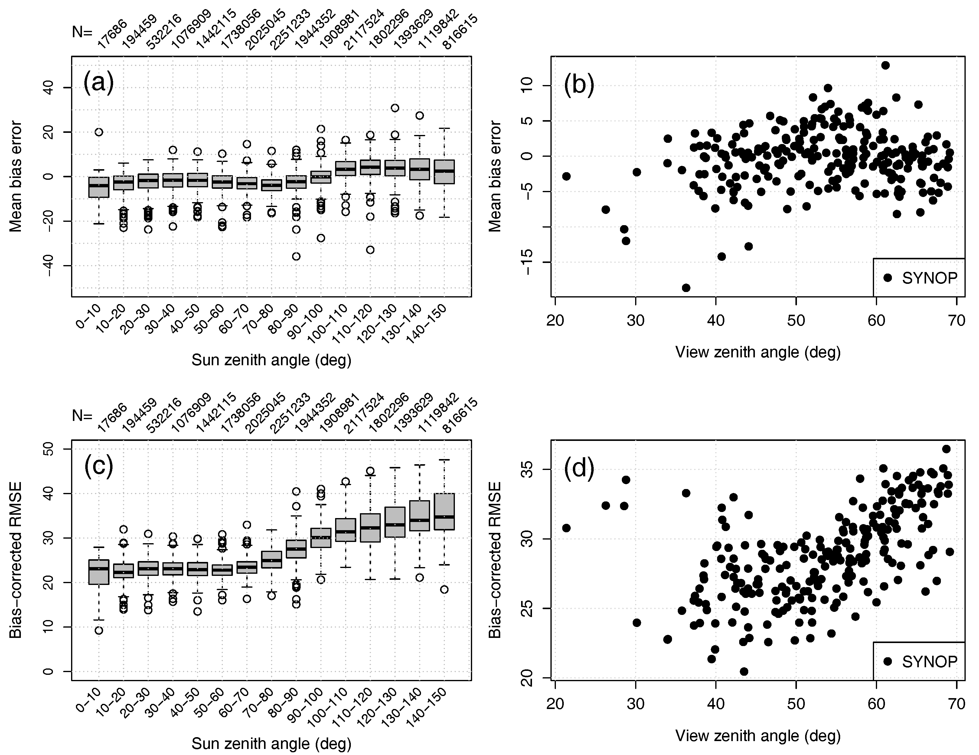
COMET slightly overestimates SYNOP CFC (MBE = 3%) and is less precise (bcRMSE = 34%) during night-time. It underestimates SYNOP CFC during daytime (MBE = −2.74%) but with higher precision (bcRMSE = 24%). It is confirmed by a more detailed performance assessment of COMET in dependence on sun zenith angle (Figure 4a,c).

A seasonal cycle of COMET performance is revealed by a negative bias and larger bcRMSE during the Northern Hemisphere’s winter months (DJF), and a positive bias and lower bcRMSE in summer months (JJA) (Table 2). The impact of seasons may be diminished, as statistics are averaged over both hemispheres; however, the greater impact of snow cover on cloud detection is expected to occur in the Northern Hemisphere.

Table 3. Performance statistics of level-2 COMET CFC as compared with synoptic observations at 237 sites for the winter season (December–February) for different climatic zones and illumination conditions.

	Day		Night		Twilight
	MBE	bcRMSE	MBE	bcRMSE	MBE	bcRMSE
Cold	−7.22	28.96	−4.43	41.37	−7.95	35.63
Temperate	−3.31	24.32	2.33	34.40	−1.77	30.17
Arid	−5.15	24.27	2.63	31.71	−2.70	27.94
Tropical	−12.19	26.34	3.12	34.11	−10.30	30.03
Ocean	−8.41	26.60	−0.15	32.74	−8.10	28.59

which presents COMET performance for the Northern Hemisphere winter months only, reveals the most prominent underestimation of CFC in Tropical areas (exceeding −10%). However, the impact of this underestimation on the overall COMET performance is limited due to a small number of synoptic observations available in the tropical zone (see N in Table 2). The seasonal cycle of COMET performance with larger negative bias during DJF is related to the expected major problems with cloud detection over snow-covered surfaces. The lowest precision (bcRMSE >40%) for the night-time retrieval in the Cold zone reveals a limited cloud detection capability over snow-covered surfaces, when only one thermal channel is available.

On average, at low viewing zenith angles (VZA < 30°), COMET underestimates SYNOP CFC by approximately 7% (Table 3). This dependency is due to the very few long-term SYNOP sites in the arid zone of Africa located at a low viewing angle and is discussed later in this section. At VZA > 60 degrees, COMET loses precision (Figure 4b,d) as expected due to high atmospheric path lengths and possibly parallax effects.

Averaged over all 237 reference SYNOP sites, COMET fulfils the optimal accuracy and precision requirements (Table 1) for both daily and monthly means. The optimal accuracy requirements are 1% for MBE met by daily (MBE = −0.17%) and monthly (MBE = −0.14%) COMET CFC means. Similarly, bcRMSE of 16.53% and 7.04% comply with optimal precision requirements of 25% and 15% for daily and monthly means, respectively (Table 2). Taking accuracy and precision requirements simultaneously into account—optimal, target and threshold requirements are met by 26%, 80% and 97% of sites, respectively (Figure 5).

CFC at six sites do not comply with the threshold requirements (Figure 5). For the SYNOP station with the WMO identifier 17,096 located in Anatolia, COMET CFC is overestimated. This is likely related to the already described general overestimation for this region (Figure 3) and needs further analysis.

On the other hand, there are five sites where COMET underestimates SYNOP CFC by 10–20%. All five sites are located in the coastal zones of arid and oceanic environments (Figure 3). This underestimation is consistent with Table 2 summarizing the statistics for these environments. We hypothesize that the underestimation is related to a scale mismatch at coastal zones where the observation site is located on land and the satellite pixel covers both ocean and land. Possibly, the sharp change in background (clear-sky) reflectance and brightness temperature within a single satellite pixel might not be compatible with the current CFC algorithm where several continuous cloud scores as input to the naïve Bayesian classifier are based on difference tests between the all-sky and clear-sky reflectance fields. Eventually, the cloud cover itself has a sharp change from land to ocean, leading to a reference measurement on land which is not representative for the entire satellite pixel. These hypotheses need to be verified and taken into account in the algorithm improvements for a next release of COMET.

Decadal Stability

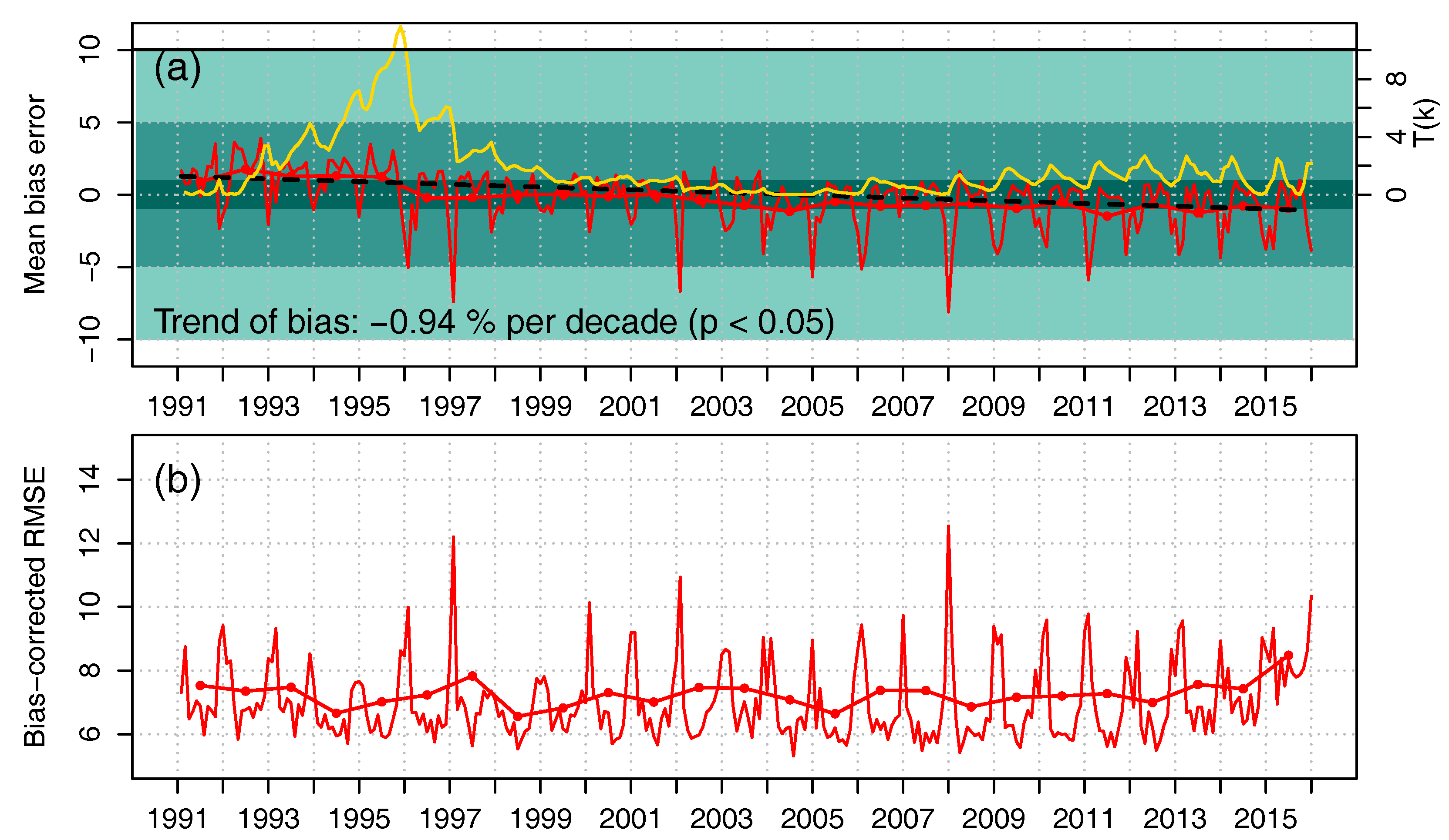
To assess the temporal stability of COMET, we computed MBE and bcRMSE for each month in 1991–2015 over 237 SYNOP sites. As shown by a dashed line in Figure 6a, the trend in the bias is −0.94% per decade, thus within the optimal requirements. Note that this negative trend is related to the overestimation of SYNOP CFC before 1996, i.e., no significant trend was detected separately for years before and after 1996.

The break in the MBE time series was corroborated by the relative SNHT test which, following the guidelines of Aguilar et al. [45] and Toreti et al. [46], was carried out based on the de-trended mean monthly cloud fraction difference between COMET and SYNOP. 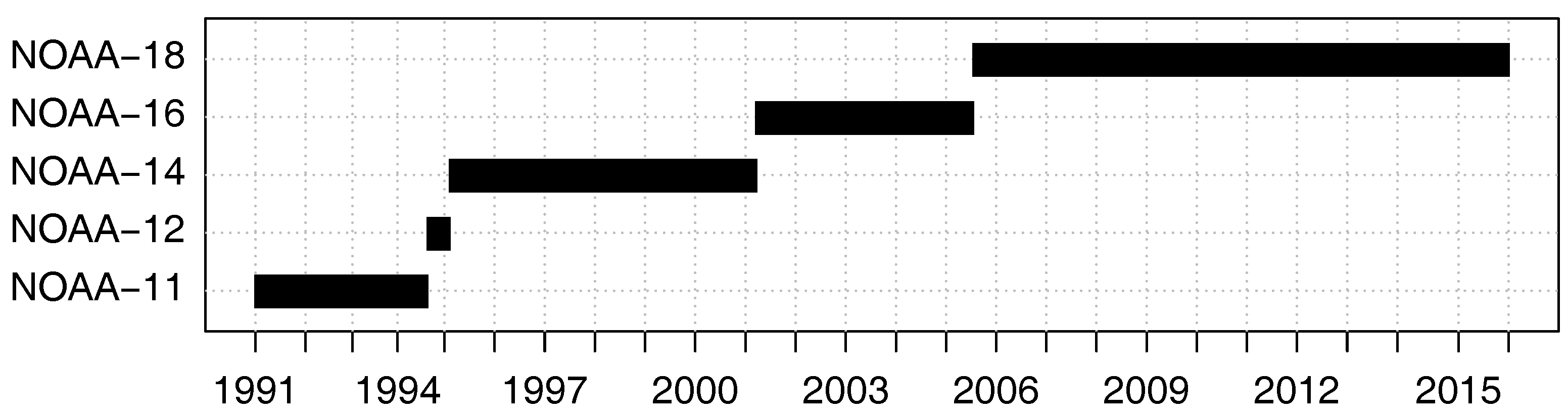At the turn of 1995 and 1996, statistic $T\left(k\right)$ of the relative test slightly exceeds the critical value, which for a time series of 300 elements is equal 10.02 at the 95% confidence level (see Appendix A.2 for SNHT definition and details). The explanation for this inhomogeneity, very likely caused by non-climatic factors, is not trivial, as there was no change of satellites in that period (see Figure 1). We intend to evaluate possible inhomogeneities in both the reference and satellite time series separately in order to better attribute the source of this inhomogeneity.

The homogeneity analysis does not reveal a break during the transfer from MFG/MVIRI to MSG/SEVIRI (2004 to 2005). Differences in COMET employing MVIRI and SEVIRI might still be present at locations where synoptic observations are not available (e.g., ocean regions). Therefore, a more extensive comparison of monthly mean MVIRI- and SEVIRI-based CFC was carried out during 2005 at the 1° × 1° resolution within 60°N/S–60°W/E.

Over all grids, CFC from MFG is on average 0.43% lower than CFC from MSG (

Table 4. Comparison statistics of gridded CFC derived by Meteosat First Generation (MFG) and Meteosat Second Generation (MSG) for 2005.

	N	MBE	bcRMSE
MFG—MSG (all months)	153,384	−0.43	2.26
MFG—MSG (January)	12,782	−0.50	2.33
MFG—MSG (June)	12,782	0.04	2.63

). A similar difference is revealed for January, whereas for June the mean difference is close to 0%. Yet, the differences are not equally distributed in space. For both months, MSG CFC is 5–10% greater than MFG CFC at the Arabian Sea (Figure 7c,d). Concurrently, close to the African coast around 10°S–20°S (a region of tropical marine stratocumulus), MFG CFC has up to 25% larger values in June than MSG. Unfortunately, these differences in ocean regions can neither be evaluated against synoptic observations, as these are not available, nor against CALIPSO/CALIOP launched only in 2006. Therefore, COMET must be used with caution when analysing cloud cover in a tropical marine stratocumulus area where climate models have been shown to have difficulties in simulating the magnitude as well as the variability of albedo.

6. Validation with CALIPSO-CALIOP

The validation against CALIPSO/CALIOP was performed for the entire year of 2010. It required the spatial and temporal matching of observations from SEVIRI (used in COMET for 2010) and CALIOP. Collocations were computed using spatial nearest neighbour search and scan line-based time matching. Maximum collocation distances were 5 km and 7.5 min in space and time.

Due to the advanced lidar technique, CALIOP is much more sensitive to high and optically thin clouds than SEVIRI. Therefore, not only did we compare COMET against the uppermost cloud layer detected by CALIOP, but also against CALIOP data filtered by means of the cloud optical thickness (COT). The latter can tell us more about how accurate COMET is relative to the potential of the SEVIRI sensor.

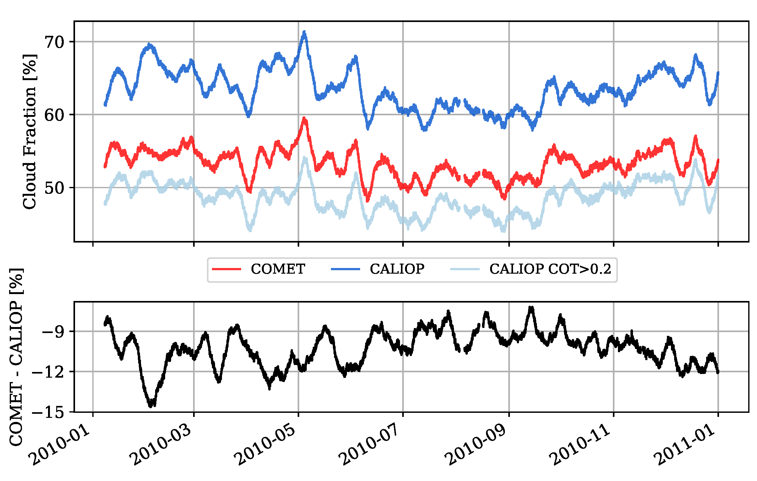
We derived two binary CALIOP cloud masks by interpreting CALIOP measurements with total column COT > 0 and COT > 0.2 as cloudy. To be comparable with CALIOP, COMET CFC was converted to a binary cloud mask by setting CFC > 55% to cloudy and CFC ≤ 55% to clear sky. CALIOP cloud mask of COT > 0 is expected to contain thin clouds which are more likely to be missed for COMET due to the sensitivity of the SEVIRI sensor. Thus, the threshold used for the second cloud mask (COT > 0.2) should improve the agreement of COMET and CALIOP. Cloud detection sensitivity, defined as the minimum cloud optical thickness for which 50% of clouds could be detected, is 0.225 for AVHRR as recently estimated by Karlsson and Håkansson [47]. This is close to the threshold applied in our evaluation.

Figure 8 shows a time series of the cloud fraction from COMET and CALIOP at all collocations in 2010. Meteosat underestimates CFC as compared to CALIOP (COT > 0.0) and overestimates as compared to CALIOP (COT > 0.2). The underestimation is expected as a passive sensor reveals lower sensitivity to thin clouds. The fluctuation of MBE revealed at the bottom panel of Figure 8 needs to be further investigated. The following

Table 5. Summary of validation results for the COMET-based cloud mask against CALIOP. ‘Clr’ stands for clear, and ‘cld’ for cloudy. Day/Night threshold is at a solar zenith angle of 80 degrees. All values in percent (0–100).

	CALIOP COT > 0.0					CALIOP COT > 0.2
	All	Day	Night	Sea	Land	All	Day	Night	Sea	Land
POD clr	86.38	88.20	84.37	85.64	88.12	80.18	81.46	78.76	79.06	82.29
FAR clr	32.10	30.24	34.13	31.78	32.55	11.88	9.39	14.61	12.01	11.59
POD cld	76.31	75.55	77.01	77.57	73.75	88.60	89.75	87.63	89.10	87.55
FAR cld	9.38	9.08	9.64	9.55	9.05	19.08	20.07	18.20	19.19	18.93
Hit rate	80.01	80.48	79.55	80.41	79.23	84.28	85.20	83.38	84.06	84.73
KSS	62.70	63.75	61.38	63.03	61.87	68.79	71.21	66.39	68.16	69.84
MBE	−9.99	−10.31	−9.68	−9.11	−11.69	4.62	5.54	3.72	5.10	3.71
bcRMSE	43.58	42.96	44.18	43.31	44.04	39.38	38.07	40.59	39.60	38.90

summarizes the performance of COMET over all collocations (denoted as All), as well as for different subsets related to light conditions and land–ocean mask. Averaged over all months and collocations, COMET bias is of −9.99% which is within the threshold requirements. Probability of cloud detection is consistent above 70% for all subsets. However, COMET has a higher probability to incorrectly detect clear sky during night-time (${\mathrm{FAR}}_{\mathrm{clr}}$ = 34.13%) compared to daytime (${\mathrm{FAR}}_{\mathrm{clr}}$ = 30.24%). Yet, MBE (in absolute terms) is lower for night-time observations. Cloud detection is very similar in terms of accuracy and precision over land and sea.

We also analysed the impact of excluding clouds with COT smaller than a certain threshold from the CALIPSO-based cloud mask. In Figure 9, the probability of detection increases with the COT threshold used to distinguish clear and cloudy CALIOP measurements. However, it does not imply that optically thinner clouds than, say COT = 0.1, cannot be detected by SEVIRI, because the false alarm ratio also increases with the COT threshold. It is more likely to miss a cloud with SEVIRI, if it is optically thin. Thus, there are two effects happening simultaneously when increasing the CALIOP COT threshold (Figure 9). First, optically thin CALIOP clouds not detected by SEVIRI are reset to cloud-free, hence the cloud POD increases. Second, optically thin CALIOP clouds detected by SEVIRI are reset to cloud-free, leading to an increased False Alarm Ratio. The coupling of these effects causes the Hitrate and KSS to peak at COT of 0.15.

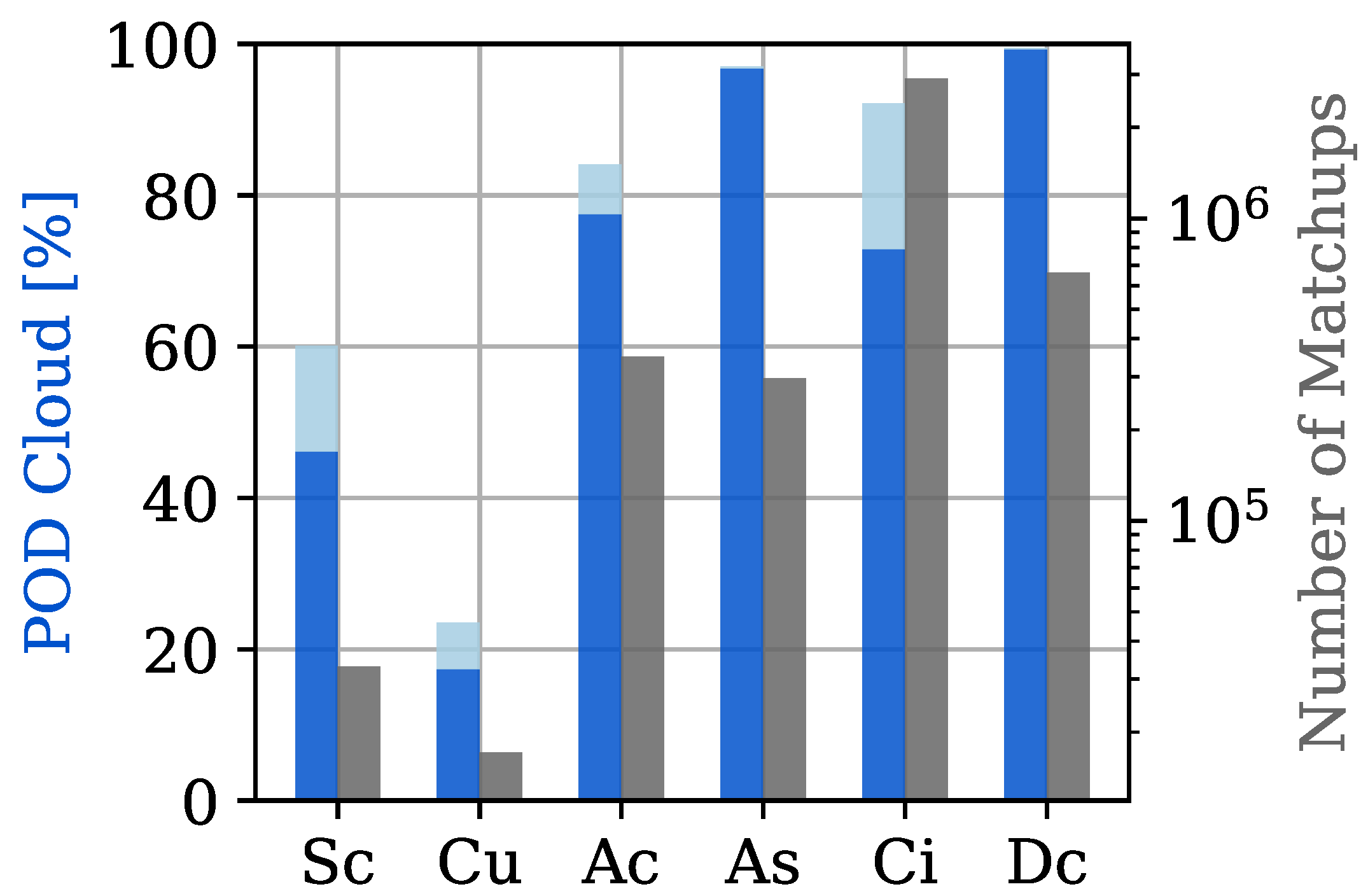
The contribution of different CALIOP cloud types to the probabilities of cloud detection are shown in Figure 10. It should be noted that cloud analyses with respect to the CALIOP cloud type have a very strong ice cloud bias. It is found that CALIOP provides a cloud type classification for 98% of the ice clouds, but only for 30% of the liquid clouds.

Altostratus and deep convective clouds are detected with almost 100% probability by COMET, and Altocumulus almost reaches the precision requirements of 90%. Cirrus clouds narrowly miss the threshold requirements. However, when ignoring CALIOP measurements with total column COT < 0.2, Cirrus detection meets the target requirements. Transition Stratocumulus clouds are detected with a probability of 60% for COT > 0.2. Concurrently, only 20% of low, broken Cumulus clouds are detected regardless a threshold for COT. However, the occurrence probability for this cloud type is two orders of magnitude lower than, for example, Cirrus clouds. Low Broken cumulus especially in ocean areas (see POD in Figure 11) have a similar thermal signature as the underlying water with little spatio-temporal variance to be exploited, especially during night-time when COMET only uses the single thermal channel. The Bayesian classifier of COMET was trained with SYNOP sites which might not adequately represent this cloud type over oceanic areas.

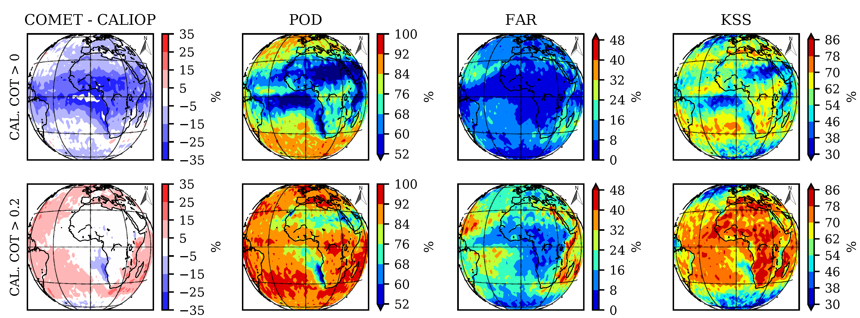
Figure 11 presents COMET performance statistics over Meteosat disc remapped to a regular 1.5° × 1.5° grid. Mean annual COMET and CALIOP CFC (with COT > 0) reveal similar spatial patterns, however with COMET underestimating CALIOP over the Atlantic Ocean within 0–10°N as well as for the tropics over Africa. This can be explained by a significant contribution of Cirrus clouds (in the tropics) and broken Cumulus clouds (over the ocean), which can be missed by COMET. This underestimation is indeed no longer visible when CALIOP CFC is estimated using COT > 0.2, thus excluding optically thin clouds. Probability of detection exceeds 90% over large areas, i.e., Northern and Southern Atlantic Ocean, South America, Europe and South Africa. Two main spots of lower POD are located over the Atlantic Ocean around 10°S–0°, Western Indian Ocean, as well as over desert (Sahara and Arabian Peninsula).

7. Intercomparison with Other Satellite Datasets

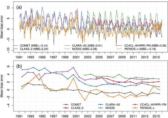
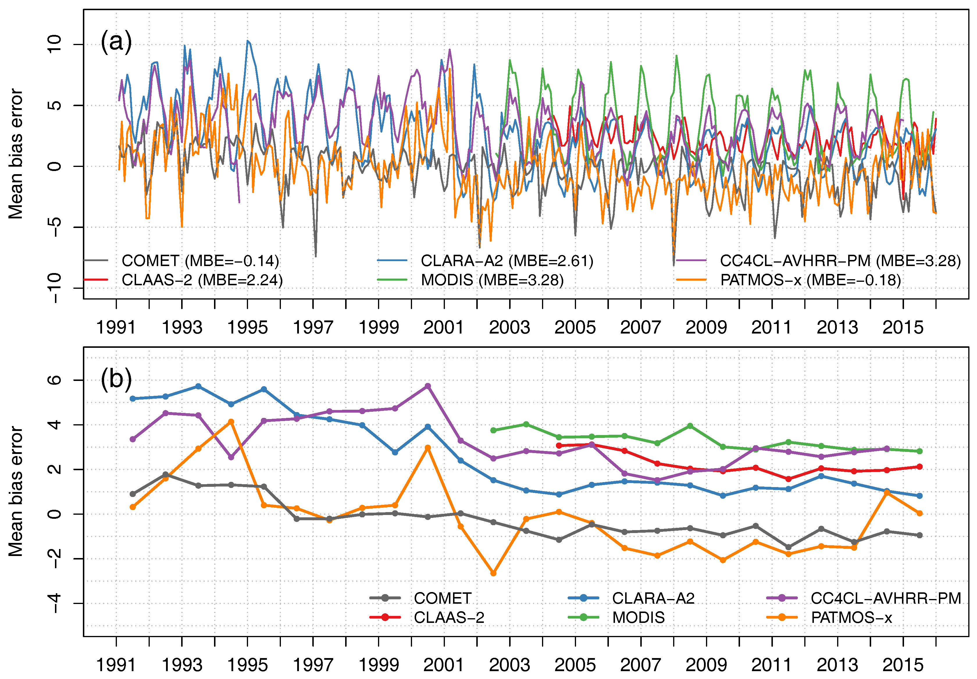
Figure 12 reveals COMET’s closest correspondence to SYNOP among all intercompared datasets. The MBE of COMET is −0.14% while the majority of others exceeds 2%. The MBE of PATMOS-x is as low as −0.18%, but it has to be noted that only collocations (of time difference below 10 min) of instantaneous level-2 COMET and PATMOS-x observations were aggregated to monthly means, while the other intercomparisons are based on level-3. Moreover, the stability of COMET’s MBE over time appears to be best when compared to other long-term climatologies of PATMOS-x, CLARA-A2 and CC4CL-AVHRR-PM.

All datasets including COMET perform best for summer months. However, COMET has inversed annual seasonality of MBE with a negative bias in winter and a positive one in summer. So, while traditional remote sensing cloud cover datasets often falsely identify snow surfaces as clouds, COMET underestimates cloud cover above bright and cold surfaces. COMET utilizes relative differences between the all-sky and clear-sky solar and thermal signal. These differences are low for cold and snow-covered surfaces and also for low stratus clouds which occur during winter time in continental Europe. Explicitly sharpening the Bayesian classifier of COMET for these situations might yield a lower bias during Northern Hemisphere winter months. As already shown in Table 3, this is also related to underestimation during daytime and twilight, with most negative MBE in the tropics.

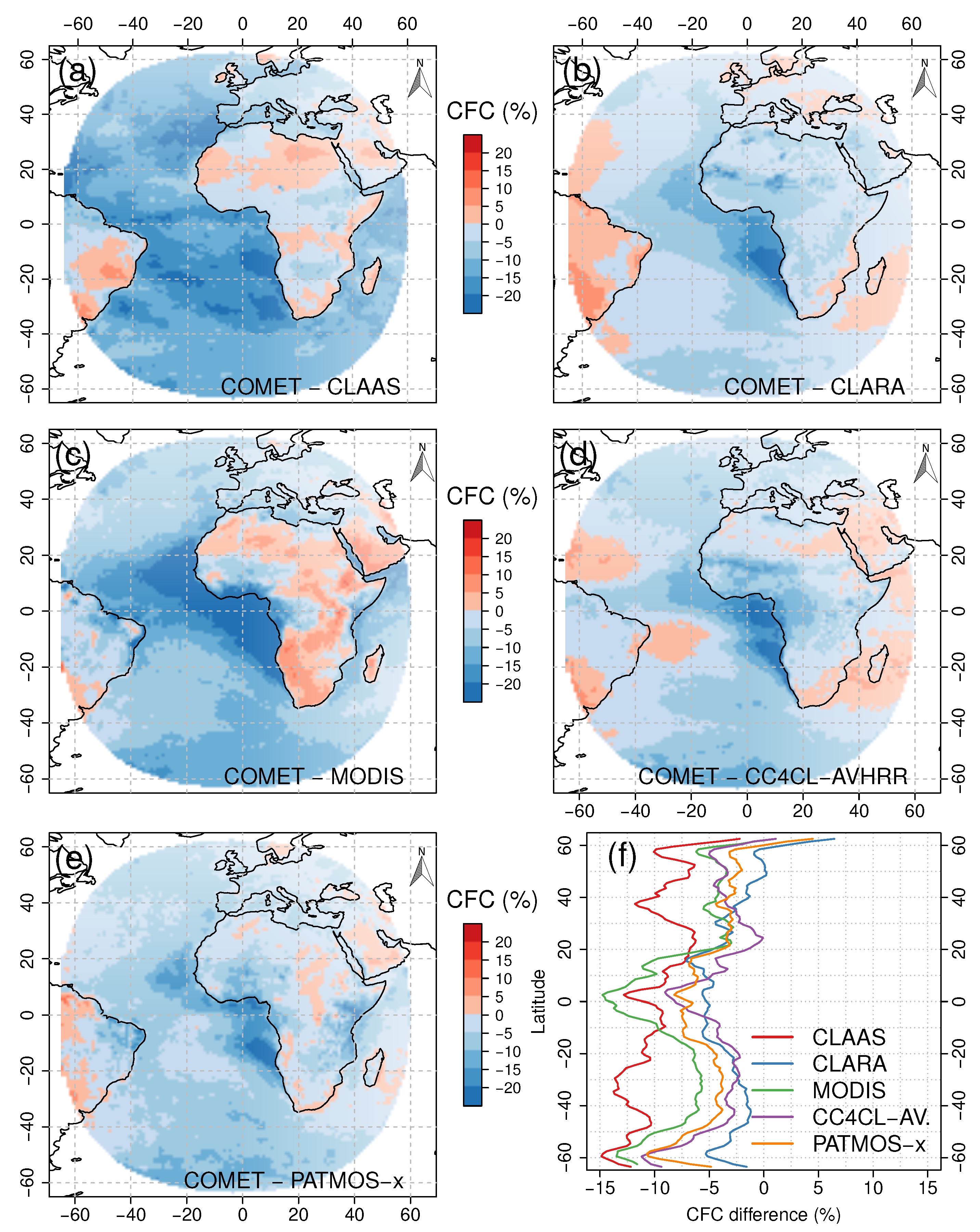
When all CDRs are compared over the whole Meteosat scanning area, COMET reveals similarity to AVHRR-based records CLARA-A2, CC4CL-AVHRR and PATMOS-x (

Table 6. Evaluation of COMET versus CLAAS-2, CLARA-A2, MODIS, CC4CL-AVHRR and PATMOS-x for 2005 averaged over the Meteosat disc.

	N	MBE	bcRMSE
COMET—CLAAS-2	158,508	−9.99	11.85
COMET—CLARA-A2	158,508	−4.03	6.41
COMET—MODIS	158,424	−8.17	10.21
COMET—CC4CL-AVHRR	158,508	−4.78	7.51
COMET—PATMOS-x	158,508	−5.69	7.14

). In both cases, COMET detects around 4–5% less clouds. Spatial distribution of the differences is similar for both comparisons (Figure 13b,d). CLARA-A2 and CC4CL-AVHRR CFCs are greater than COMET’s for most of the Meteosat disc with maxima close to the African coast around 10°–20°S (a region of tropical marine stratocumulus).

Differences of COMET versus MODIS and CLAAS-2 are larger (Table 6). COMET underestimates MODIS and CLAAS-2 by 8% and 10%, respectively. In both cases, there is a tendency to COMET’s overestimation over land (Africa) and underestimation over the Ocean (Figure 13a,c).

8. Conclusions and Outlook

The recently released CM SAF cloud fractional cover climate data record (COMET) derived from MVIRI and SEVIRI on board two generations of geostationary Meteosat satellites has been presented. Our study demonstrates that two Meteosat heritage channels (i.e., broadband visible and thermal) allow for cloud fractional cover estimates at native sensor resolution of older MVIRI sensors (i.e., every 30 min at 5 km resolution) that fulfil high requirements defined by the climate community. As compared to synoptic observations, COMET with −0.15% of mean bias error and 7.04% of bias-corrected root mean square error complies with GCOS’ optimal requirements. However, COMET CFC reveals lower performance during night-time (when only thermal information is available) as well as for high viewing angles (i.e., beyond approximately 55 degrees). Further, our evaluation exposes limitations of cloud detection in winter months (December–February). Still, COMET CFC reveals optimal temporal stability (trend in bias) of −0.94% per decade, which is best among the analysed long-term CFC climate data records (i.e., CLARA-A2, and CC4CL-AVHRR-PM).

COMET’s excellent performance builds on new intercalibrations of Meteosat heritage channels as well as a novel cloud detection methodology. The fundamental climate data records (i.e., time series of intercalibrated radiances and brightness temperature) have been carefully developed with the stable HIRS measurements as a reference for MVIRI WV and IR. A major novelty of the COMET cloud detection method is the modelling of clear-sky background fields using the Meteosat data itself, and not using the external auxiliary data. It exploits the high temporal resolution of geostationary sensors in a parametric analysis of the clear sky diurnal cycle instead of dealing with each time step separately. A second novelty is an application of continuous cloud mask scores that are used to derive CFC by means of a machine learning approach (naïve Bayesian classifier). The classifier is trained towards synoptic observations, which guarantees a good correspondence of COMET CFC and SYNOP. We claim that our satellite retrievals can complement or replace the synoptic observations with a huge advantage of being available at every grid point and with high frequency.

It is planned to extend COMET for the second edition with precedent years (1983–1990) covered by MVIRI sensors on board Meteosat-2 and Meteosat-3 upon the availability of new intercalibration coefficients, and prolonged with the period 2015–2021. The algorithm should then be improved to solve the limitations pinpointed in this study (e.g., inhomogeneity 1995/1996, cloud detection over snow and at coastal zones). In addition, a training set which consisted of synoptic observations on land, could be enhanced with global data of CALIPSO/CALIOP [47]. Further, the new release should follow the metrological norms on providing uncertainties of climate variables [48].

The COMET data record provides information on cloud occurrence which is indispensable for Meteosat-based derivation of other climate variables released by CM SAF, i.e., Land SUrface Temperature dataset from METeosat First and Second Generation (SUMET, https://doi.org/10.5676/EUM_SAF_CM/LST_METEOSAT/V001). It also provides data that allow for climate analysis of trends and variability of cloudiness and its daily cycle in the last three decades (e.g., [49]). Notwithstanding, COMET CFC can be of interest to a broader community than satellite data producers and climate scientists only. This includes anyone requiring high temporal resolution cloud fraction estimates as input for further studies, for example, in the domains of model data assimilation, solar energy, ecology or tourism.

References

1. Stephens, G.L. Cloud Feedbacks in the Climate System: A Critical Review. J. Clim. 2005, 18, 237–273. [Google Scholar] [CrossRef]
2. Boucher, O.; Randall, D.; Artaxo, P.; Bretherton, C.; Feingold, G.; Forster, P.; Kerminen, V.M.V.M.; Kondo, Y.; Liao, H.; Lohmann, U.; et al. Clouds and Aerosols. In Climate Change 2013: The Physical Science Basis. Contribution of Working Group I to the Fifth Assessment Report of the Intergovernmental Panel on Climate Change; Intergovernmental Panel on Climate Change: Geneva, Switzerland, 2013. [Google Scholar]
3. Zelinka, M.D.; Klein, S.A.; Taylor, K.E.; Andrews, T.; Webb, M.J.; Gregory, J.M.; Forster, P.M. Contributions of different cloud types to feedbacks and rapid adjustments in CMIP5. J. Clim. 2013, 26, 5007–5027. [Google Scholar] [CrossRef]
4. GCOS-138. Implementation Plan for the Global Observing System for Climate in Support of the UNFCCC; Technical Report; World Meteorological Organisation: Geneva, Switzerland, 2010. [Google Scholar]
5. GCOS-200. The Global Observing System for Climate: Implementation Needs; Technical Report; World Meteorological Organisation: Geneva, Switzerland, 2016. [Google Scholar]
6. GCOS-154. Systematic Observation Requirements for Satellite-Based Products for Climate, 2011 Update: Supplemental Details to the Satellite-Based Component of the Implementation Plan for the Global Observing System for Climate in Support of the UNFCCC; Technical Report; Global Climate Observing System: Geneva, Switzerland, 2011. [Google Scholar]
7. Rossow, W.B.; Schiffer, R.A. Advances in Understanding Clouds from ISCCP. Bull. Am. Meteorol. Soc. 1999, 80, 2261–2287. [Google Scholar] [CrossRef]
8. Young, A.H.; Knapp, K.R.; Inamdar, A.; Hankins, W.; Rossow, W.B. The International Satellite Cloud Climatology Project H-Series Climate Data Record Product. Earth Syst. Sci. Data Discuss. 2017, 1–21. [Google Scholar] [CrossRef]
9. Heidinger, A.K.; Foster, M.J.; Walther, A.; Zhao, X. The pathfinder atmospheres-extended AVHRR climate dataset. Bull. Am. Meteorol. Soc. 2014, 95, 909–922. [Google Scholar] [CrossRef]
10. Karlsson, K.G.; Anttila, K.; Trentmann, J.; Stengel, M.; Fokke Meirink, J.; Devasthale, A.; Hanschmann, T.; Kothe, S.; Jaäskelaïnen, E.; Sedlar, J.; et al. CLARA-A2: The second edition of the CM SAF cloud and radiation data record from 34 years of global AVHRR data. Atmos. Chem. Phys. 2017, 17, 5809–5828. [Google Scholar] [CrossRef]
11. Stengel, M.; Stapelberg, S.; Sus, O.; Schlundt, C.; Poulsen, C.; Thomas, G.; Christensen, M.; Carbajal Henken, C.; Preusker, R.; Fischer, J.; et al. Cloud property datasets retrieved from AVHRR, MODIS, AATSR and MERIS in the framework of the Cloud_cci project. Earth Syst. Sci. Data Discuss. 2017, 9, 881–904. [Google Scholar] [CrossRef]
12. Hollmann, R.; Merchant, C.J.; Saunders, R.; Downy, C.; Buchwitz, M.; Cazenave, A.; Chuvieco, E.; Defourny, P.; de Leeuw, G.; Forsberg, R.; et al. The ESA Climate Change Initiative: Satellite Data Records for Essential Climate Variables. Bull. Am. Meteorol. Soc. 2013, 94, 1541–1552. [Google Scholar] [CrossRef] [Green Version]
13. Devasthale, A.; Karlsson, K.G.; Quaas, J.; Grassl, H. Correcting orbital drift signal in the time series of AVHRR derived convective cloud fraction using rotated empirical orthogonal function. Atmos. Meas. Tech. 2012, 5, 267–273. [Google Scholar] [CrossRef]
14. Evan, A.T.; Heidinger, A.K.; Vimont, D.J. Arguments against a physical long-term trend in global ISCCP cloud amounts. Geophys. Res. Lett. 2007, 34, L04701. [Google Scholar] [CrossRef]
15. Benas, N.; Finkensieper, S.; Stengel, M.; Van Zadelhoff, G.J.; Hanschmann, T.; Hollmann, R.; Meirink, J.F. The MSG-SEVIRI-based cloud property data record CLAAS-2. Earth Syst. Sci. Data 2017, 9, 415–434. [Google Scholar] [CrossRef]
16. Kothe, S.; Pfeifroth, U.; Cremer, R.; Trentmann, J.; Hollmann, R. A satellite-based sunshine duration climate data record for Europe and Africa. Remote Sens. 2017, 9, 429. [Google Scholar] [CrossRef]
17. Urbain, M.; Clerbaux, N.; Ipe, A.; Tornow, F.; Hollmann, R.; Baudrez, E.; Blazquez, A.V.; Moreels, J. The CM SAF TOA radiation data record using MVIRI and SEVIRI. Remote Sens. 2017, 9, 466. [Google Scholar] [CrossRef]
18. Schröder, M.; Roca, R.; Picon, L.; Kniffka, A.; Brogniez, H. Climatology of free-tropospheric humidity: Extension into the SEVIRI era, evaluation and exemplary analysis. Atmos. Chem. Phys. 2014, 14, 11129–11148. [Google Scholar] [CrossRef]
19. Stöckli, R.; Duguay-Tetzlaff, A.; Bojanowski, J.S.; Hollmann, R.; Fuchs, P.; Werscheck, M. CM SAF ClOud Fractional Cover dataset from METeosat First and Second Generation—Edition 1 (COMET Ed. 1); Satellite Application Facility for Climate Monitoring, EUMETSAT: Darmstadt, Germany, 2017. [Google Scholar]
20. Duguay-Tetzlaff, A.; Stöckli, R.; Bojanowski, J.; Hollmann, R. Meteosat Cloud Fractional Cover Edition 1, Product User Manual (PUM); Technical Report; Satellite Application Facility for Climate Monitoring, EUMETSAT: Darmstadt, Germany, 2017. [Google Scholar]
21. Stöckli, R.; Duguay-Tetzlaff, A.; Bojanowski, J.S.; Hollmann, R. Meteosat Cloud Fractional Cover Edition 1, Algorithm Theoretical Basis Document (ATBD); Technical Report; Satellite Application Facility for Climate Monitoring, EUMETSAT: Darmstadt, Germany, 2017. [Google Scholar]
22. Schmetz, J.; Pili, P.; Tjemkes, S.; Just, D.; Kerkmann, J.; Rota, S.; Ratier, A. An introduction to Meteosat Second Generation (MSG). Bull. Am. Meteorol. Soc. 2002, 83, 977–992. [Google Scholar] [CrossRef]
23. EUMETSAT. METEOSAT VIS CHANNEL CALIBRATION INFORMATION; Technical Report; EUMETSAT: Darmstadt, Germany, 2010. [Google Scholar]
24. Govaerts, Y.M.; Clerici, M.; Clerbaux, N. Operational calibration of the Meteosat radiometer VIS band. IEEE Trans. Geosci. Remote Sens. 2004, 42, 1900–1914. [Google Scholar] [CrossRef]
25. Deneke, H.M.; Roebeling, R.A. Downscaling of METEOSAT SEVIRI 0.6 and 0.8 μm channel radiances utilizing the high-resolution visible channel. Atmos. Chem. Phys. 2010, 10, 9761–9772. [Google Scholar] [CrossRef] [Green Version]
26. Stöckli, R.; Bojanowski, J.S.; Duguay-Tetzlaff, A.; Viju, J. Climatological Cloud Detection with Heritage Geostationary Satellite Sensors. J. Geophys. Res. 2018. in preparation. [Google Scholar]
27. Khlopenkov, K.V.; Trishchenko, A.P. SPARC: New Cloud, Snow, and Cloud Shadow Detection Scheme for Historical 1-km AVHHR Data over Canada. J. Atmos. Ocean. Technol. 2007, 24, 322–343. [Google Scholar] [CrossRef]
28. Heidinger, A.K.; Evan, A.T.; Foster, M.J.; Walther, A. A Naive Bayesian Cloud-Detection Scheme Derived from CALIPSO and Applied within PATMOS-x. J. Appl. Meteorol. Climatol. 2012, 51, 1129–1144. [Google Scholar] [CrossRef]
29. CM SAF. Product Requirements Document SAF/CM/DWD/PRD/2.8; Technical Report; EUMETSAT Satellite Application Facility on Climate Monitoring: Darmstadt, Germany, 2014. [Google Scholar]
30. GCOS-107. Systematic Observation Requirements for Satellite-Based Products For Climate; Technical Report GCOS-107, WMO-TD No. 1338; Global Climate Observing System: Geneva, Switzerland, 2006. [Google Scholar]
31. Winker, D.M.; Vaughan, M.A.; Omar, A.; Hu, Y.; Powell, K.A.; Liu, Z.; Hunt, W.H.; Young, S.A. Overview of the CALIPSO Mission and CALIOP Data Processing Algorithms. J. Atmos. Ocean. Technol. 2009, 26, 2310–2323. [Google Scholar] [CrossRef]
32. Vaughan, M.A.; Powell, K.A.; Winker, D.M.; Hostetler, C.A.; Kuehn, R.E.; Hunt, W.H.; Getzewich, B.J.; Young, S.A.; Liu, Z.; McGill, M.J. Fully Automated Detection of Cloud and Aerosol Layers in the CALIPSO Lidar Measurements. J. Atmos. Ocean. Technol. 2009, 26, 2034–2050. [Google Scholar] [CrossRef]
33. MODIS Atmosphere L3 Monthly Product; Technical Report; NASA MODIS Adaptive Processing System, Goddard Space Flight Center: Greenbelt, MD, USA, 2015. Available online: https://modaps.modaps.eosdis.nasa.gov/services/about/products/c6/MOD08_M3.html (accessed on 21 May 2018).
34. CM SAF. Validation Report of CM SAF Cloud, Albedo, Radiation Data Record, AVHRR-Based, Edition 2 (CLARA-A2); Technical Report SAF/CM/SMHI/VAL/GAC/CLD/2, Issue 2.0; EUMETSAT Satellite Application Facility on Climate Monitoring: Darmstadt, Germany, 2016. [Google Scholar]
35. CM SAF. Validation Report of CM SAF SEVIRI Cloud Products Edition 2 (CLAAS-2); Technical Report SAF/CM/KNMI/VAL/SEV/CLD/2, Issue 2.0; EUMETSAT Satellite Application Facility on Climate Monitoring: Darmstadt, Germany, 2016. [Google Scholar]
36. Heidinger, A.; Goldberg, M.; Jelenak, A.; Pavolonis, M. A New AVHRR Cloud Climatology; Proc. SPIE 5658; SPIE: Bellingham, WA, USA, 2005; Volume 197. [Google Scholar]
37. Pavolonis, M.; Heidinger, A.; Uttal, T. Daytime Global Cloud Typing from AVHRR and VIIRS: Algorithm Description, Validation, and Comparisons. J. Appl. Meteorol. 2005, 44, 804–826. [Google Scholar] [CrossRef]
38. Thomas, S.; Heidinger, A.; Pavolonis, M. Comparison of NOAA’s operational AVHRR-derived cloud amount to other satellite-derived cloud climatologies. J. Clim. 2004, 17, 4805–4822. [Google Scholar] [CrossRef]
39. Bojanowski, J.S.; Stöckli, R.; Tetzlaff, A.; Kunz, H. The Impact of Time Difference between Satellite Overpass and Ground Observation on Cloud Cover Performance Statistics. Remote Sens. 2014, 6, 12866–12884. [Google Scholar] [CrossRef]
40. McGarragh, G.R.; Poulsen, C.A.; Thomas, G.E.; Povey, A.C.; Sus, O.; Stapelberg, S.; Schlundt, C.; Proud, S.; Christensen, M.W.; Stengel, M.; et al. The Community Cloud retrieval for CLimate (CC4CL). Part II: The optimal estimation approach. Atmos. Meas. Tech. Discuss. 2017, 2017, 1–55. [Google Scholar] [CrossRef]
41. Sus, O.; Stengel, M.; Stapelberg, S.; McGarragh, G.; Poulsen, C.; Povey, A.C.; Schlundt, C.; Thomas, G.; Christensen, M.; Proud, S.; et al. The Community Cloud retrieval for Climate (CC4CL). Part I: A framework applied to multiple satellite imaging sensors. Atmos. Meas. Tech. Discuss. 2017, 2017, 1–42. [Google Scholar] [CrossRef]
42. Poulsen, C.A.; Siddans, R.; Thomas, G.E.; Sayer, A.M.; Grainger, R.G.; Campmany, E.; Dean, S.M.; Arnold, C.; Watts, P.D. Cloud retrievals from satellite data using optimal estimation: Evaluation and application to ATSR. Atmos. Meas. Tech. 2012, 5, 1889–1910. [Google Scholar] [CrossRef]
43. Stapelberg, S.; Stengel, M.; Karlsson, K.G.; Meirink, J.F.; Bojanowski, J.; Hollmann, R. ESA Cloud_cci Product Validation and Intercomparison Report (PVIR). Technical Report; Issue 4, rev. 1, 19 April 2017 edn. Available online: http://www.esa-cloud-cci.org/?q=documentation (accessed on 21 May 2018).
44. Peel, M.C.; Finlayson, B.L.; Mcmahon, T.A. Updated world map of the Koppen-Geiger climate classification. HESSD Earth Syst. Sci. Discuss. 2007, 4, 439–473. [Google Scholar] [CrossRef]
45. Aguilar, E.; Auer, I.; Brunet, M.; Peterson, T.C.; Wieringa, J. Guidance on metadata and homogenization; Technical Report, WMO TD N. 1186 (WCDMP N. 53); World Meteorological Organization: Geneva, Switzerland, 2003. [Google Scholar]
46. Toreti, A.; Kuglitsch, F.G.; Xoplaki, E.; Della-Marta, P.; Aguilar, E.; Prohom, M.; Luterbacher, J. A note on the use of the standard normal homogeneity test to detect inhomogeneities in climatic time series. Int. J. Climatol. 2011, 31, 630–632. [Google Scholar] [CrossRef]
47. Karlsson, K.G.; Håkansson, N. Detailed characterisation of AVHRR global cloud detection performance of the CM SAF CLARA-A2 climate data record based on CALIPSO-CALIOP cloud information. Atmos. Meas. Tech. Discuss. 2017, 2017, 1–28. [Google Scholar] [CrossRef]
48. Merchant, C.J.; Paul, F.; Popp, T.; Ablain, M.; Bontemps, S.; Defourny, P.; Hollmann, R.; Lavergne, T.; Laeng, A.; de Leeuw, G.; et al. Uncertainty information in climate data records from Earth observation. Earth Syst. Sci. Data Discuss. 2017, 1–28. [Google Scholar] [CrossRef]
49. Pfeifroth, U.; Bojanowski, J.S.; Clerbaux, N.; Manara, V.; Sanchez-Lorenzo, A.; Trentmann, J.; Walawender, J.P.; Hollmann, R. Satellite-based trends of solar radiation and cloud parameters in Europe. Adv. Sci. Res. 2018, 15, 31–37. [Google Scholar] [CrossRef]
50. Wilks, D.S. Statistical Methods in the Atmospheric Sciences, 2nd ed.; International Geophysics; Academic Press: Cambridge, MA, USA, 2006; 648p. [Google Scholar]
51. Alexandersson, H. A homogeneity test applied to precipitation data. J. Climatol. 1986, 6, 661–675. [Google Scholar] [CrossRef]
52. Khaliq, M.N.; Ouarda, T. On the critical values of the standard normal homogeneity test (SNHT). Int. J. Climatol. 2007, 27, 681–687. [Google Scholar] [CrossRef]
Figure 1. Overview of the Meteosat record used as input for the generation of COMET.
Remotesensing 10 00804 g001
Figure 2. Overview of Advanced Very High Resolution Radiometer (AVHRR) measurements used to calculate the PATMOS-x CFC monthly means.
Remotesensing 10 00804 g002
Figure 3. Performance statistics of the instantaneous COMET CFC during 1991–2015 as compared to synoptic observations at 237 sites: mean bias error (left), bias-corrected root mean square error (right).
Remotesensing 10 00804 g003
Figure 4. Performance statistics of the level-2 COMET CFC during 1991–2015 as compared to synoptic observations at 237 sites in relation to sun zenith angle (a,c) and satellite view zenith angle (b,d). Each box in the box-and-whisker plot (a,c) is generated from all level-2 COMET-SYNOP collocations (given by N) for Satellite Zenith Angle (SZA) classes given by the x-axis. Boxes denote 1st and 3rd quartiles (with thick horizontal median line). Whiskers indicate largest and lowest values within 1.5 times the interquartile range, while circles represent values beyond this.
Remotesensing 10 00804 g004
Figure 5. Performance statistics of the COMET daily (a) and monthly (b) CFC means during 1991–2015 as compared to synoptic observations at 237 sites. Shaded areas reveal the accuracy requirements.
Remotesensing 10 00804 g005
Figure 6. Time series of mean bias error (a) and bias-corrected root mean square error (b) of COMET as compared to synoptic observations at 237 sites in 1991–2015. The thick lines with dots represent annual means. The black dashed line represents a Theil–Sen linear trend provided with its Mann–Kendall statistical significance. Shaded areas reveal the accuracy requirements. A yellow solid line reveals the T ( k ) statistic from the Standard Normal Homogeneity Test.
Remotesensing 10 00804 g006
Figure 7. Comparison of COMET CFC monthly means (0–100%) of 2005 derived from Meteosat First Generation (MFG) and Meteosat Second Generation (MSG). Upper panels present COMET MFG (a) and COMET MSG (b) annual means. Lower panels show a difference bewteen COMET MFG and COMET MSG for January (c) and June (d).
Remotesensing 10 00804 g007
Figure 8. Five-day moving average of COMET and CALIPSO cloud mask (yielding a cloud fraction, top) and a difference between both (bottom).
Remotesensing 10 00804 g008
Figure 9. COMET cloud scores as a function of the COT threshold used to discriminate clear and cloudy CALIOP observations. KSS denotes the Hanssen–Kuiper’s Discriminant.
Remotesensing 10 00804 g009
Figure 10. Probability of detection for COMET cloud mask resolved by cloud type. The cloud type is taken at the CALIOP cloud layer where the top-to-bottom integrated optical thickness exceeds 0.2. Blue bars were computed by interpreting all CALIOP measurements with total column COT > 0 as cloudy. Light-blue bars were derived using COT > 0.2 as cloud criterion. Grey bars give the number of matchups by cloud type.
Remotesensing 10 00804 g010
Figure 11. Mean annual CFC of Meteosat and reference CALIOP, and skill scores derived for COT > 0 (first row) and COT > 0.2 (second row).
Remotesensing 10 00804 g011
Figure 12. Time series of monthly (a) and aggregated to yearly (b) mean bias error of COMET and intercompared satellite-based CDR as compared to synoptic observations at 237 sites. Values in brackets on panel (a) indicate mean MBE for the whole analysed period.
Remotesensing 10 00804 g012
Figure 13. Differences of COMET versus CLAAS-2 (a), CLARA-A2 (b), MODIS (c), CC4CL-AVHRR (d) and PATMOS-x (e) monthly means (in CFC 0–100%) for 2005 at 1° × 1° over Meteosat disc. Panel (f) presents annual (2005) zonal mean differences in cloud fractional cover between COMET and intercompared datasets.
Remotesensing 10 00804 g013