Hyperspectral and Multispectral Image Fusion via Deep Two-Branches Convolutional Neural Network


Abstract
:
1. Introduction
- We propose learning the mapping between LR and HR HSIs via deep learning, which is of high learning capacity, and is suitable to model the complex relationship between LR and HR HSIs.
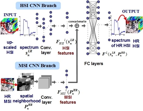
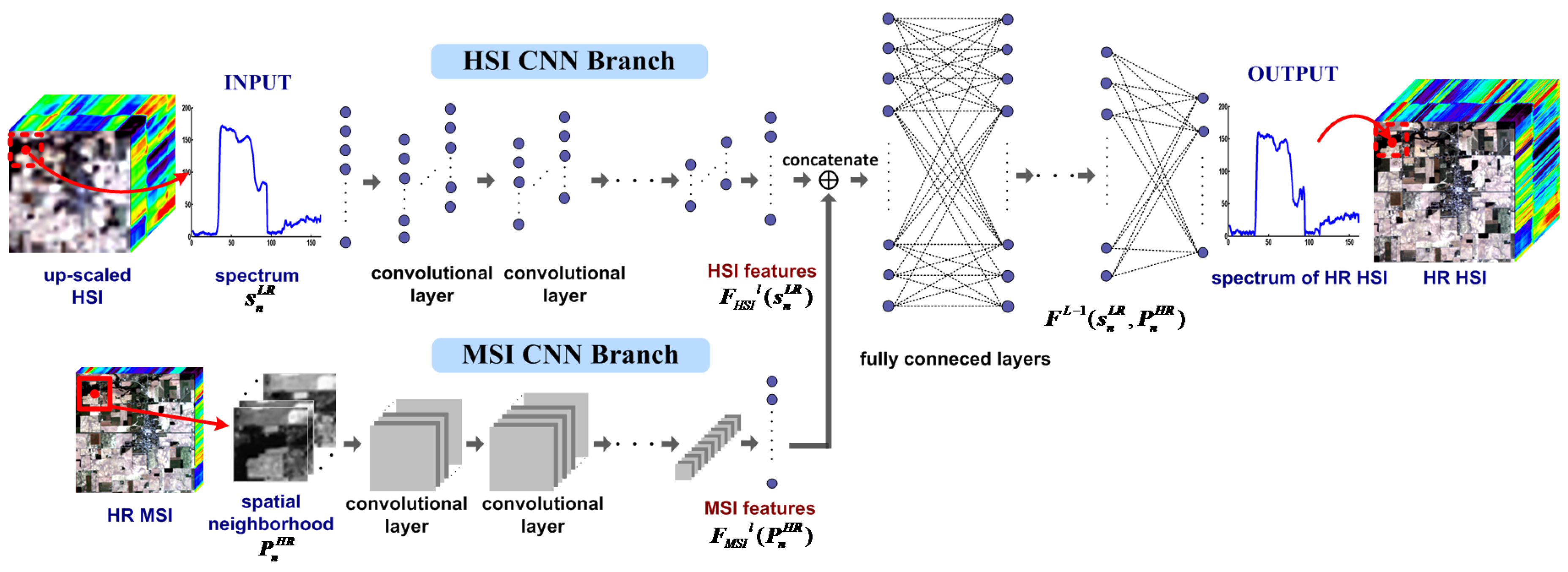
- We design a CNN with two branches extracting the features in HSI and MSI. This network could exploit the spectral correlation of HSI and fuse the information in MSI.
- Instead of reconstructing HSI in band-by-band fashion, all of the bands are reconstructed jointly, which is beneficial for reducing spectral distortion.
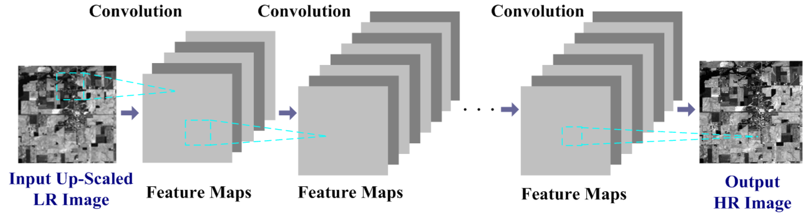
2. Background of CNN Based Image Super-Resolution
3. HSI and MSI Fusion Based on Two-Branches CNN
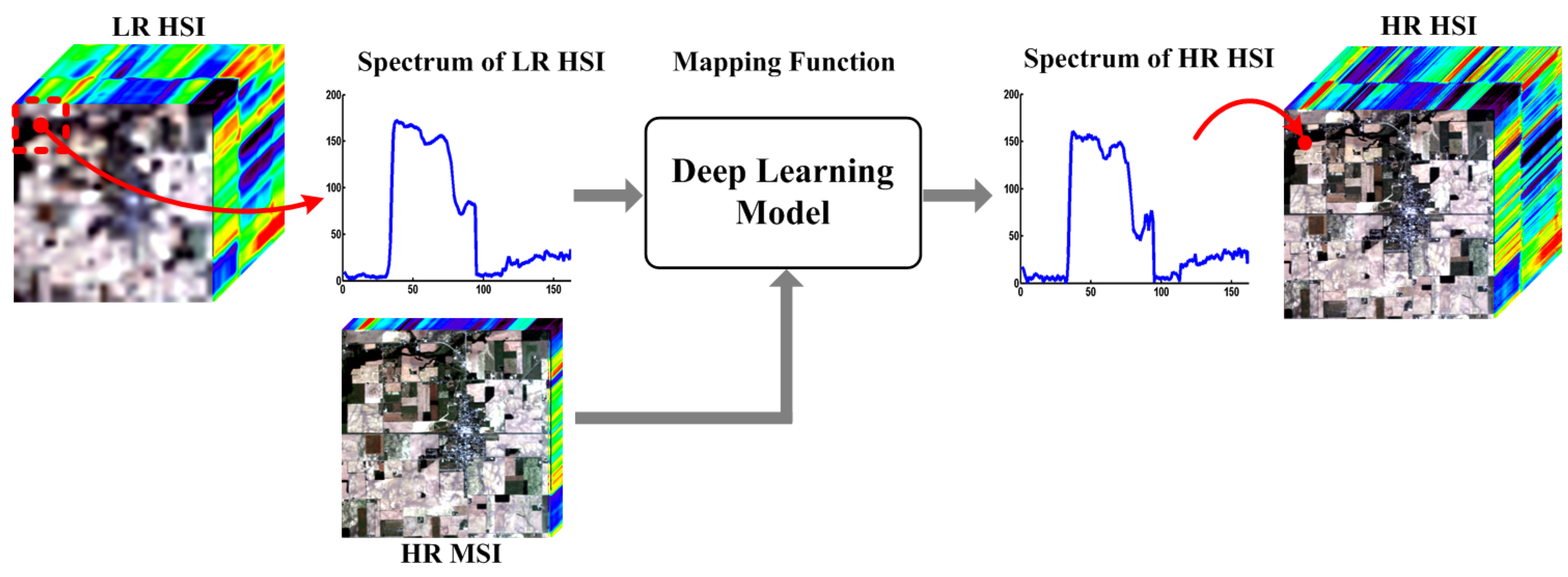
3.1. The Proposed Scheme of Deep Learning Based Fusion
3.2. Architecture of the Two Branches CNN for Fusion
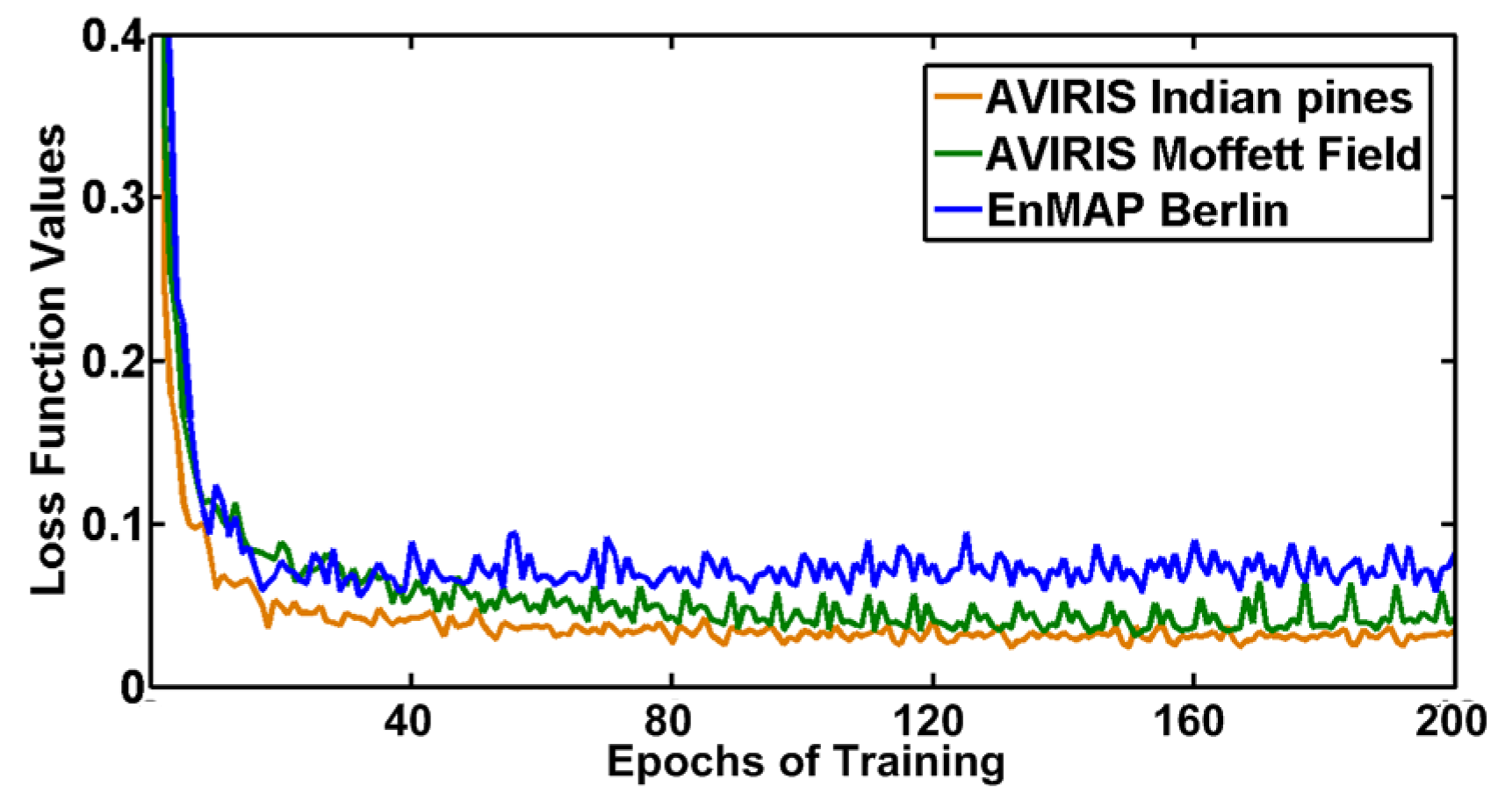
3.3. Training of the Two Branches CNN
4. Experiment Results
4.1. Experiment Setting
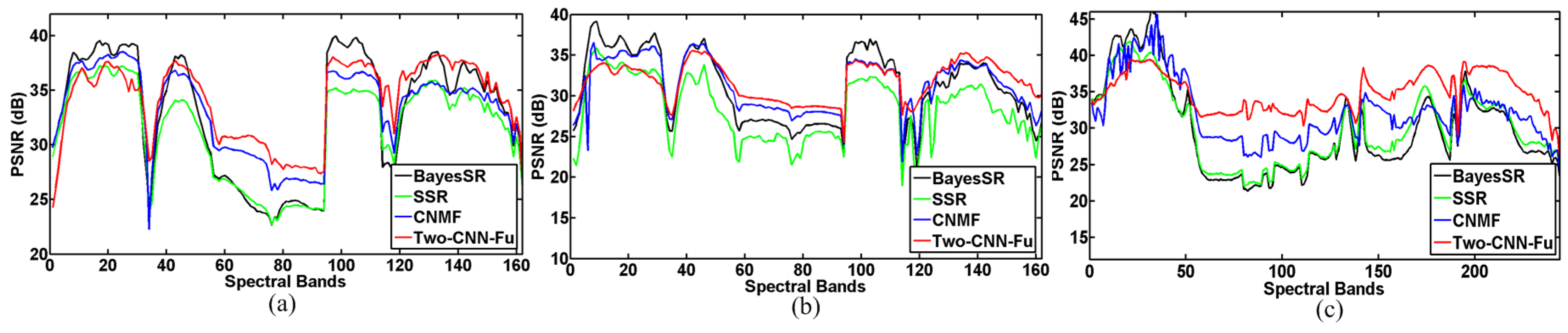
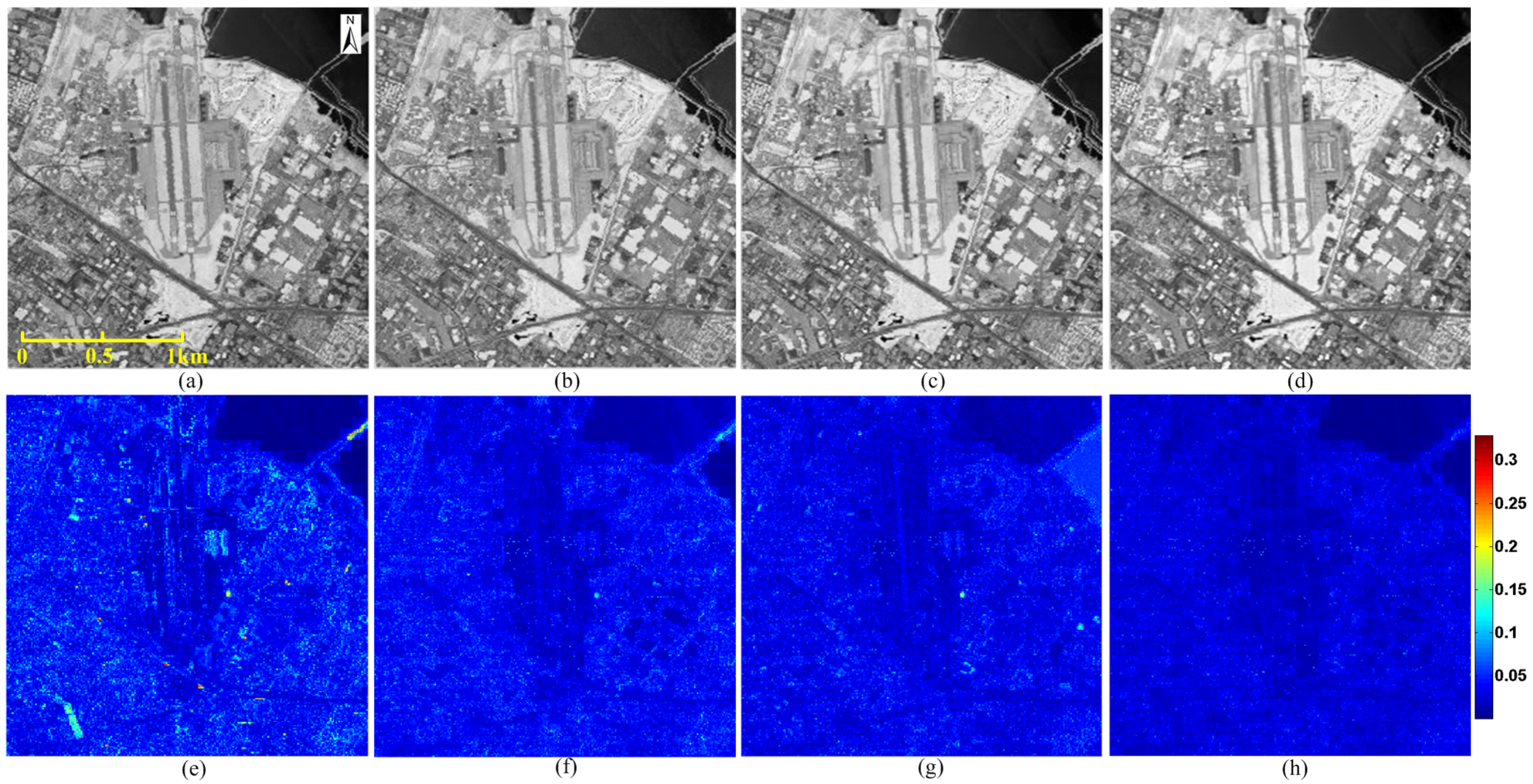
4.2. Comparison With State-of-the-Art Methods
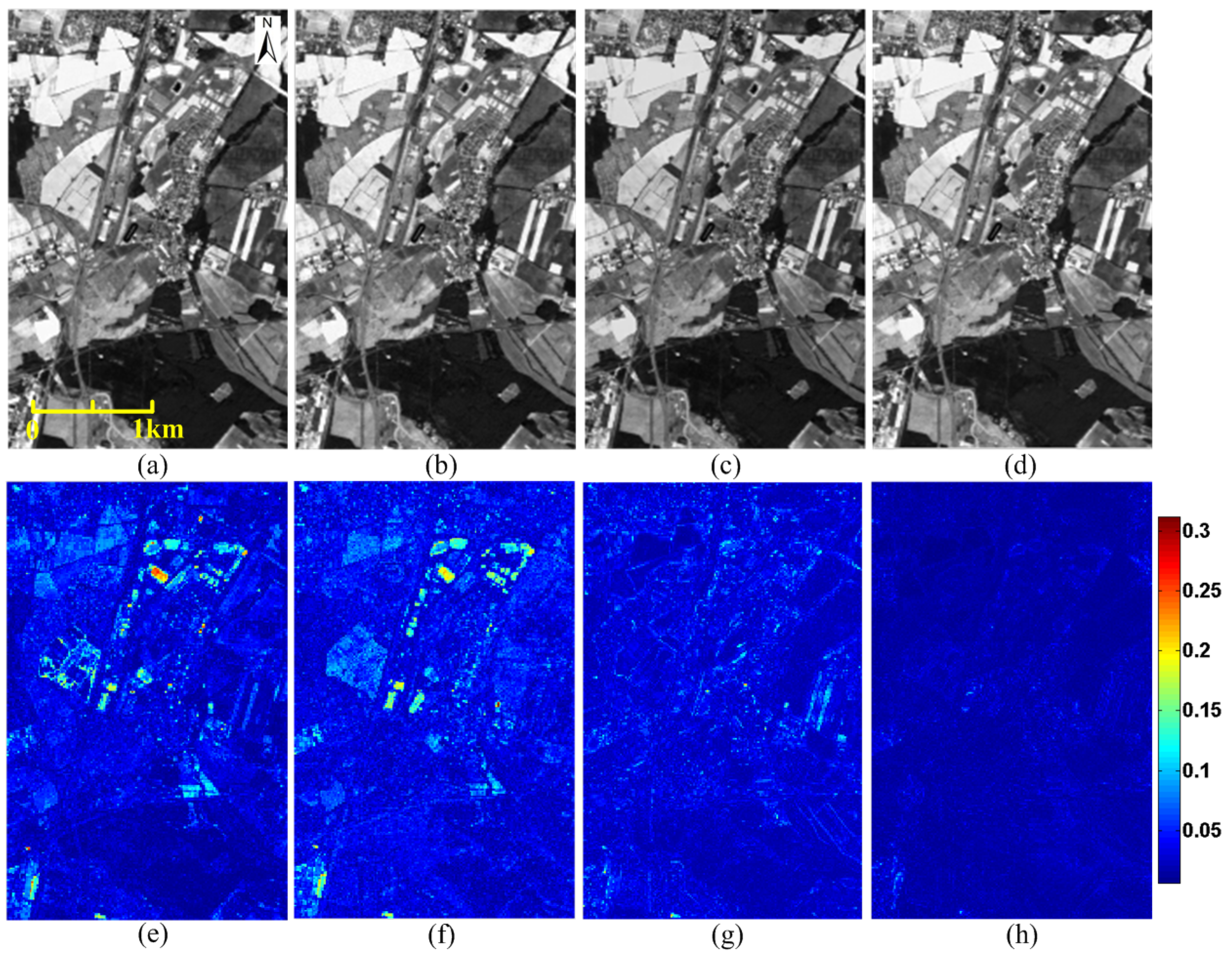
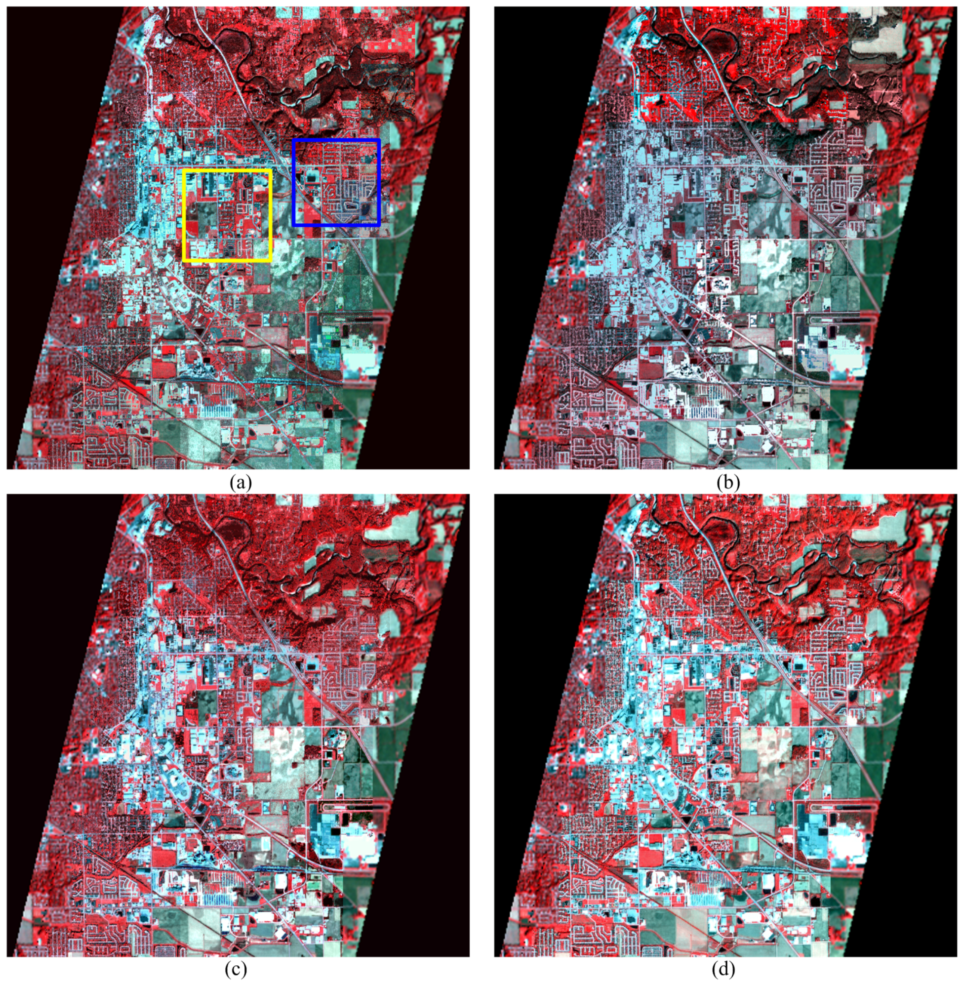
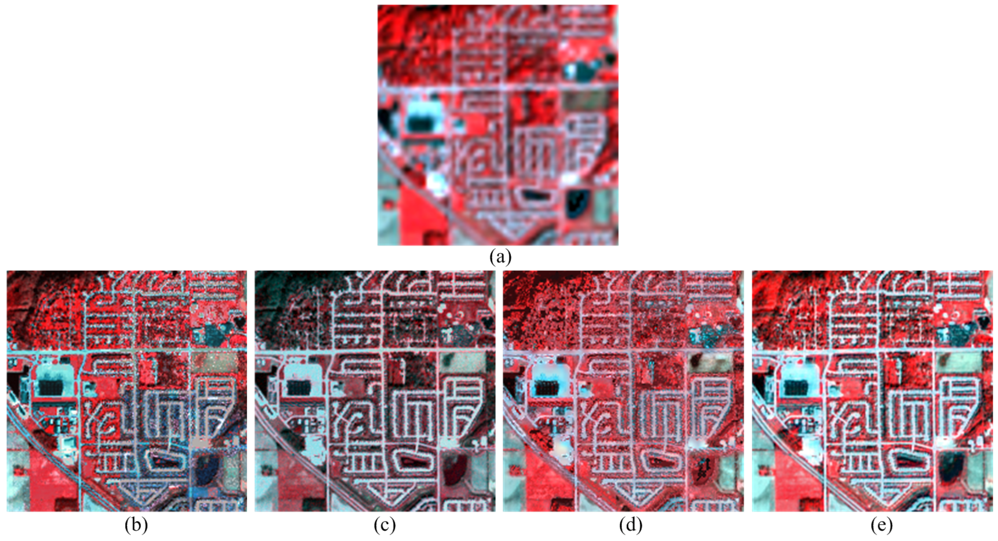
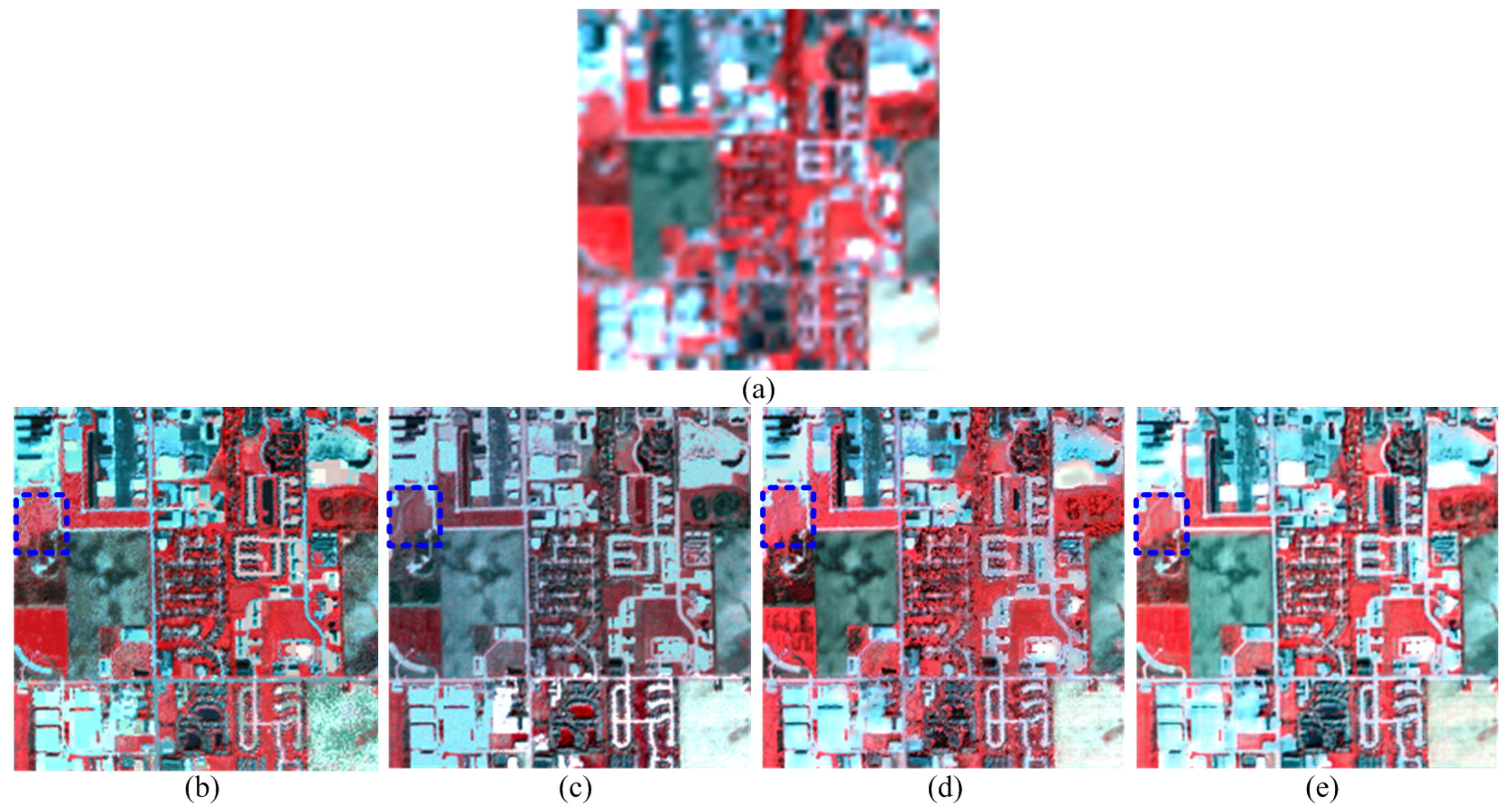
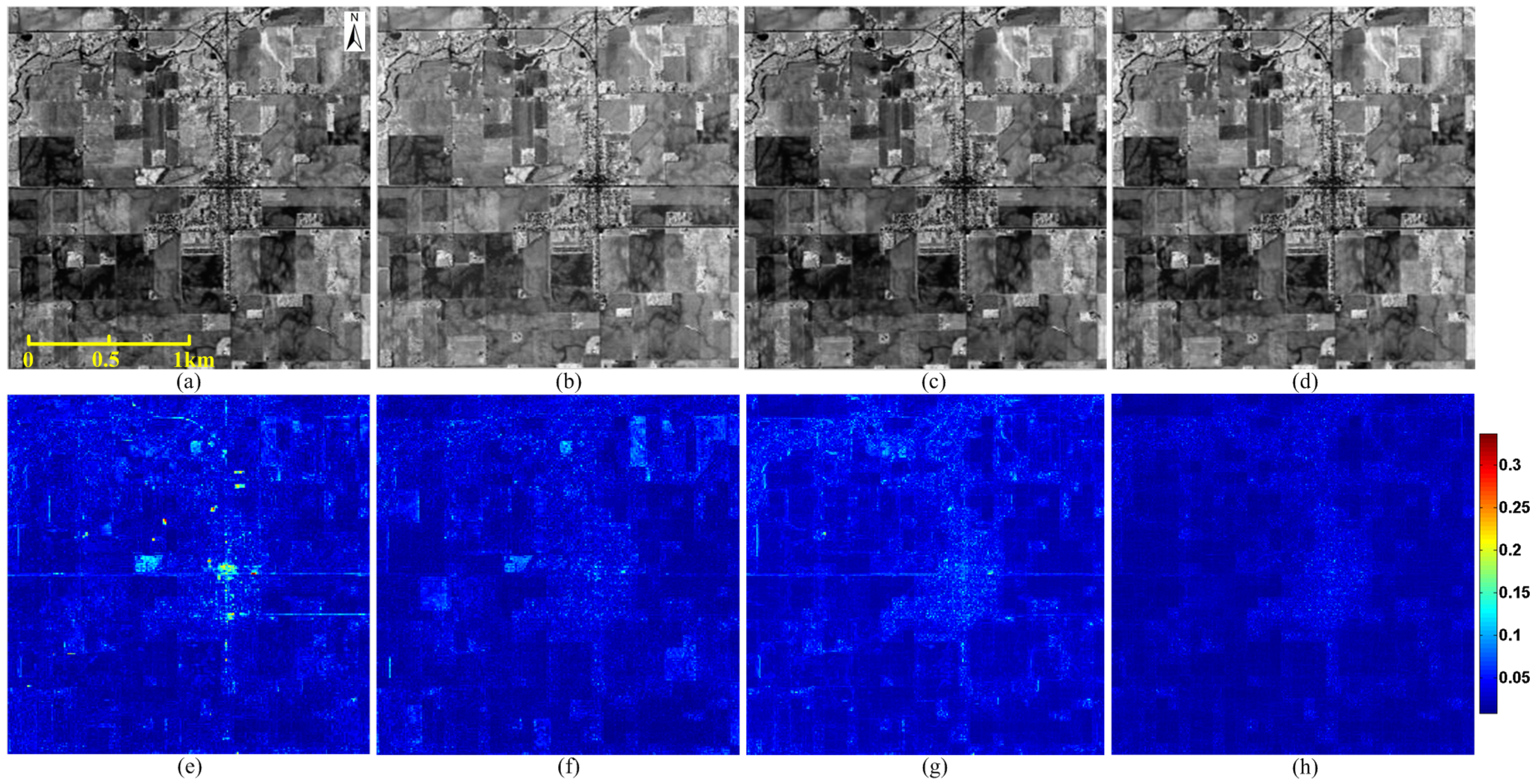
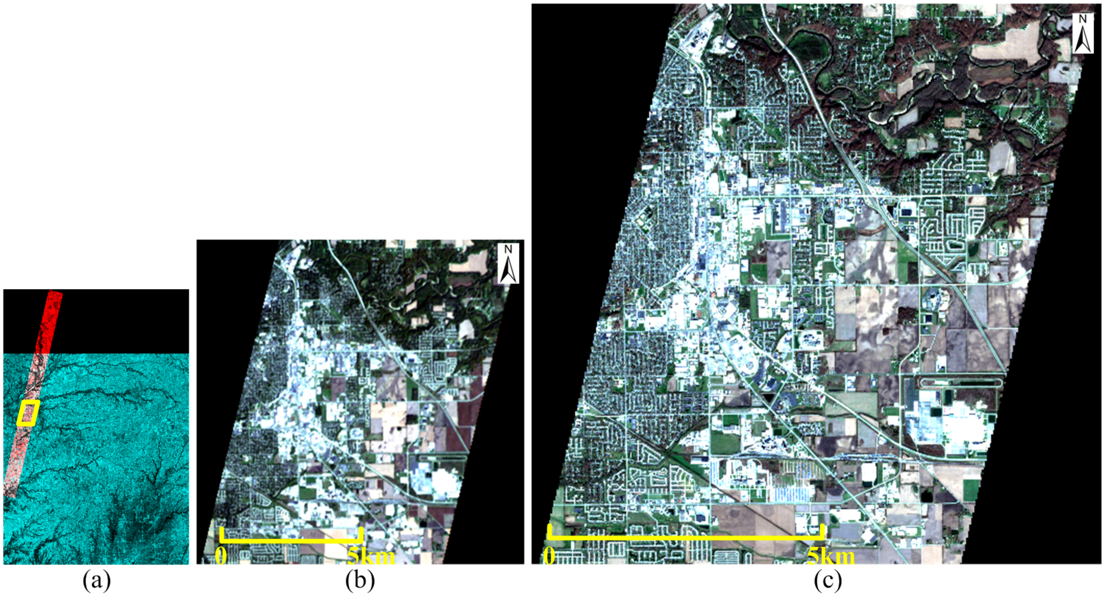
4.3. Applications on Real Data Fusion
5. Some Analysis and Discussions
5.1. Sensitivity Analysis of Network Parameters
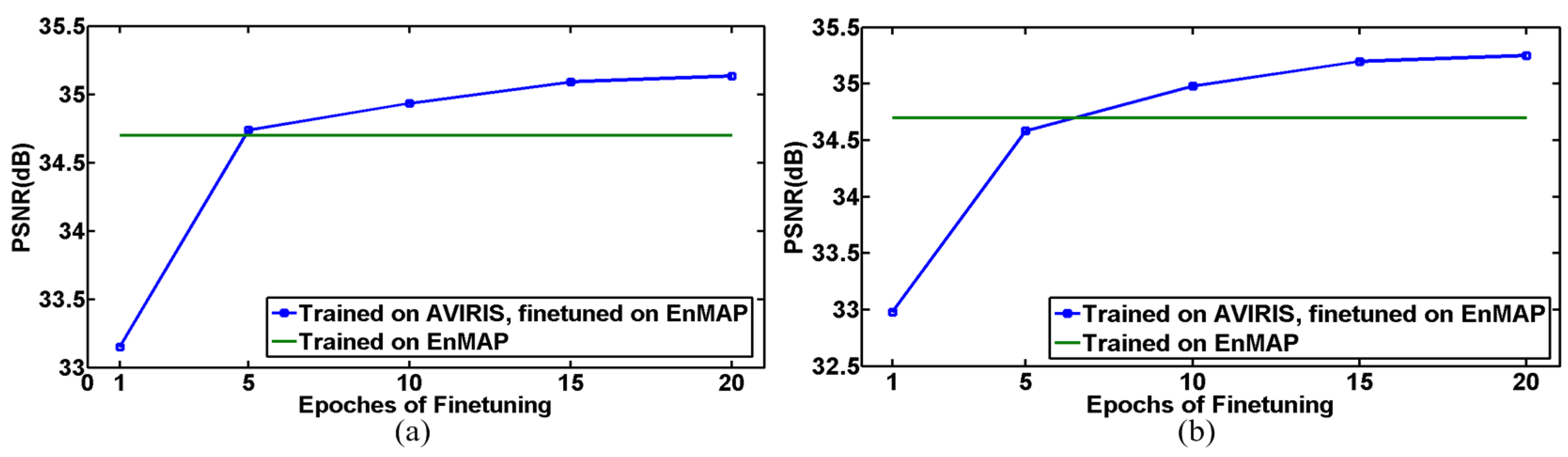
5.2. Robustness Analysis over Training Data
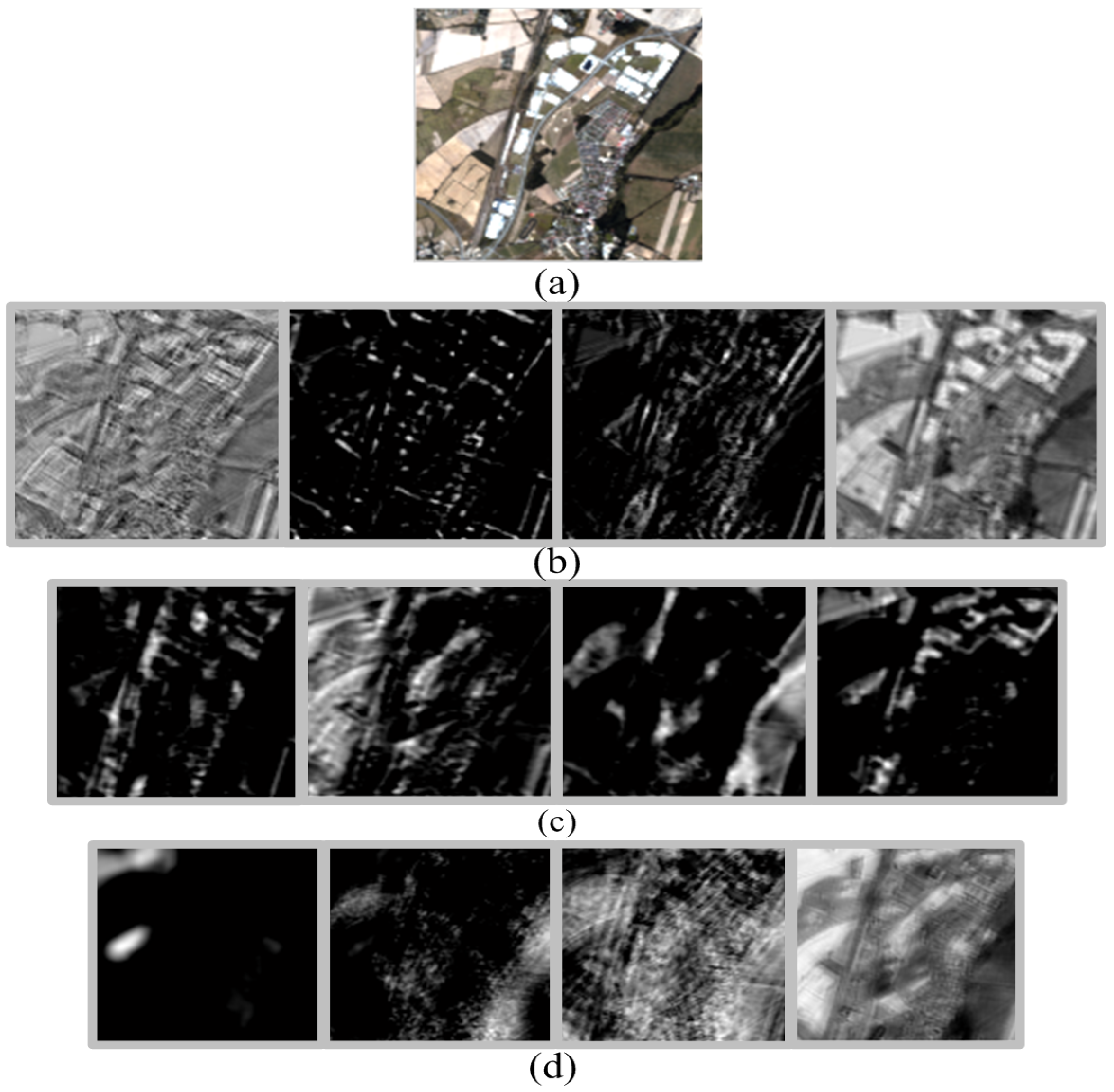
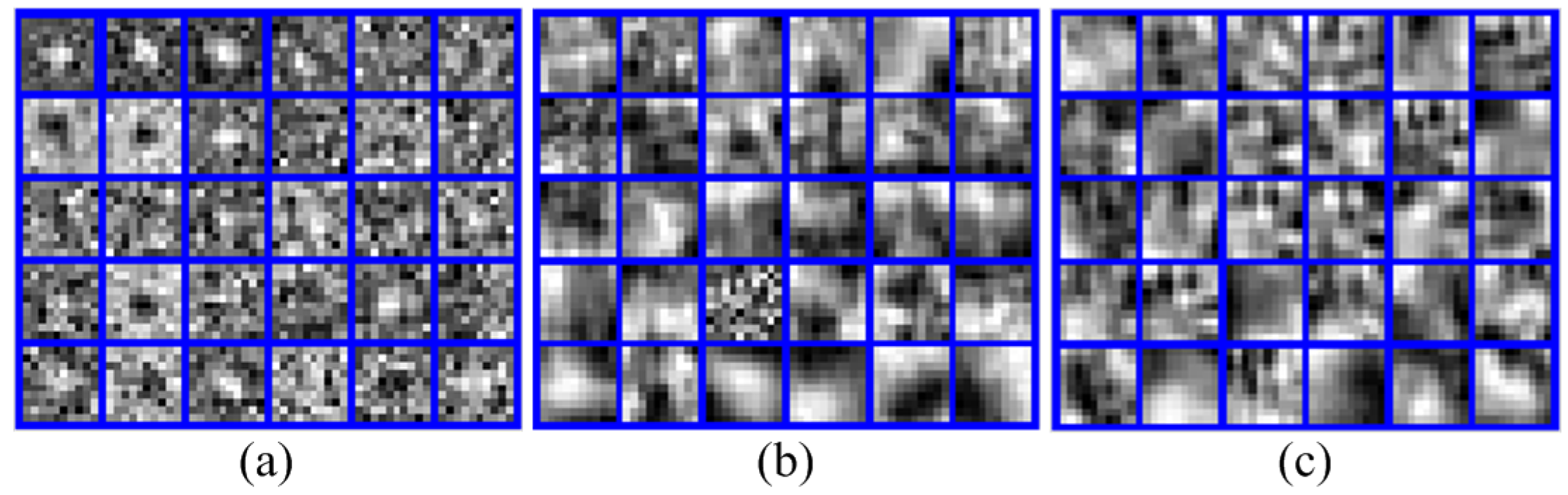
5.3. Visualization of the Extracted Features
6. Conclusions
Author Contributions
Acknowledgments
Conflicts of Interest
References
- Chang, C.I. Hyperspectral target detection. In Real-Time Progressive Hyperspectral Image Processing; Springer: New York, NY, USA, 2016. [Google Scholar]
- Yokoya, N.; Chan, J.C.W.; Segl, K. Potential of resolution-enhanced hyperspectral data for mineral mapping using simulated EnMAP and Sentinel-2 images. Remote Sens. 2016, 8, 172. [Google Scholar] [CrossRef]
- Yang, J.; Zhao, Y.Q.; Chan, J.C.W. Learning and transferring deep joint spectral-spatial features for hyperspectral classification. IEEE Trans. Geosci. Remote Sens. 2017, 55, 4729–4742. [Google Scholar] [CrossRef]
- Yokoya, N.; Grohnfeldt, C.; Chanussot, J. Hyperspectral and multispectral data fusion: A comparative review of the recent literature. IEEE Geosci. Remote Sens. Mag. 2017, 5, 29–56. [Google Scholar] [CrossRef]
- Zhu, Z.; Yin, H.; Chai, Y.; Li, Y.; Qi, G. A novel multi-modality image fusion method based on image decomposition and sparse representation. Inf. Sci. 2018, 432, 516–529. [Google Scholar] [CrossRef]
- Yokoya, N.; Yairi, T.; Iwasaki, A. Coupled nonnegative matrix factorization unmixing for hyperspectral and multispectral data fusion. IEEE Trans. Geosci. Remote Sens. 2012, 50, 528–537. [Google Scholar] [CrossRef]
- Yokoya, N.; Mayumi, N.; Iwasaki, A. Cross-calibration for data fusion of EO-1/Hyperion and Terra/ASTER. IEEE J. Sel. Top. Appl. Earth Obs. Remote Sens. 2013, 6, 419–426. [Google Scholar] [CrossRef]
- Lanaras, C.; Baltsavias, E.; Schindler, K. Hyperspectral super-resolution by coupled spectral unmixing. In Proceedings of the IEEE International Conference on Computer Vision, Santiago, Chile, 7–13 December 2015; pp. 3586–3594. [Google Scholar]
- Huang, B.; Song, H.; Cui, H.; Peng, J.; Xu, Z. Spatial and spectral image fusion using sparse matrix factorization. IEEE Trans. Geosci. Remote Sens. 2014, 52, 1693–1704. [Google Scholar] [CrossRef]
- Zhu, X.X.; Bamler, R. A sparse image fusion algorithm with application to pan-sharpening. IEEE Trans. Geosci. Remote Sens. 2013, 51, 2827–2836. [Google Scholar] [CrossRef]
- Zhu, X.X.; Grohnfeldt, C.; Bamler, R. Exploiting joint sparsity for pansharpening: The J-SparseFI algorithm. IEEE Trans. Geosci. Remote Sens. 2016, 54, 2664–2681. [Google Scholar] [CrossRef]
- Akhtar, N.; Shafait, F.; Mian, A. Sparse spatio-spectral representation for hyperspectral image super-resolution. In Proceedings of the 13th European Conference on Computer Vision, Zurich, Switzerland, 6–12 September 2014; pp. 63–78. [Google Scholar]
- Akhtar, N.; Shafait, F.; Mian, A. Bayesian sparse representation for hyperspectral image super resolution. In Proceedings of the IEEE Conference on Computer Vision and Pattern Recognition, Boston, MA, USA, 7–12 June 2015; pp. 3631–3640. [Google Scholar]
- Wei, Q.; Bioucas-Dias, J.; Dobigeon, N.; Tourneret, J.Y. Hyperspectral and multispectral image fusion based on a sparse representation. IEEE Trans. Geosci. Remote Sens. 2015, 53, 3658–3668. [Google Scholar] [CrossRef]
- Simões, M.; Bioucas-Dias, J.; Almeida, L.B.; Chanussot, J. A convex formulation for hyperspectral image superresolution via subspace-based regularization. IEEE Trans. Geosci. Remote Sens. 2015, 53, 3373–3388. [Google Scholar] [CrossRef]
- Zhang, K.; Wang, M.; Yang, S. Multispectral and hyperspectral image fusion based on group spectral embedding and low-rank factorization. IEEE Trans. Geosci. Remote Sens. 2017, 55, 1363–1371. [Google Scholar] [CrossRef]
- Eismann, M.T.; Hardie, R.C. Hyperspectral resolution enhancement using high-resolution multispectral imagery with arbitrary response functions. IEEE Trans. Geosci. Remote Sens. 2005, 43, 455–465. [Google Scholar] [CrossRef]
- Selva, M.; Aiazzi, B.; Butera, F.; Chiarantini, L.; Baronti, S. Hyper-sharpening: A first approach on SIM-GA data. IEEE J. Sel. Top. Appl. Earth Obs. Remote Sens. 2015, 8, 3008–3024. [Google Scholar] [CrossRef]
- Kwan, C.; Budavari, B.; Bovik, A.C.; Marchisio, G. Blind quality assessment of fused worldview-3 images by using the combinations of pansharpening and hypersharpening paradigms. IEEE Geosci. Remote Sens. Lett. 2017, 14, 1835–1839. [Google Scholar] [CrossRef]
- Loncan, L.; de Almeida, L.B.; Bioucas-Dias, J.M.; Briottet, X.; Chanussot, J.; Dobigeon, N.; Fabre, S.; Liao, W.; Licciardi, G.A.; Simoes, M.; et al. Hyperspectral pansharpening: A review. IEEE Geosci. Remote Sens. Mag. 2015, 3, 27–46. [Google Scholar] [CrossRef]
- Hinton, G.E.; Salakhutdinov, R.R. Reducing the dimensionality of data with neural networks. Science 2006, 313, 504–507. [Google Scholar] [CrossRef] [PubMed]
- LeCun, Y.; Bengio, Y.; Hinton, G. Deep learning. Nature 2015, 521, 436–444. [Google Scholar] [CrossRef] [PubMed]
- Zhang, L.; Zhang, L.; Du, B. Deep learning for remote sensing data: A technical tutorial on the state of the art. IEEE Geosci. Remote Sens. Mag. 2016, 4, 22–40. [Google Scholar] [CrossRef]
- Zhu, X.X.; Tuia, D.; Mou, L.; Xia, G.S.; Zhang, L.; Xu, F.; Fraundorfer, F. Deep learning in remote sensing: A review. IEEE Geosci. Remote Sens. Mag. 2017, 5, 8–36. [Google Scholar] [CrossRef]
- Chen, Y.; Lin, Z.; Zhao, X.; Wang, G.; Gu, Y. Deep learning-based classification of hyperspectral data. IEEE J. Sel. Top. Appl. Earth Obs. Remote Sens. 2014, 7, 2094–2107. [Google Scholar] [CrossRef]
- Makantasis, K.; Karantzalos, K.; Doulamis, A.; Doulamis, N. Deep supervised learning for hyperspectral data classification through convolutional neural networks. In Proceedings of the IEEE International Geoscience and Remote Sensing Symposium, Milan, Italy, 26–31 July 2015; pp. 4959–4962. [Google Scholar]
- Zhao, W.; Du, S. Spectral-spatial feature extraction for hyperspectral image classification: A dimension reduction and deep learning approach. IEEE Trans. Geosci. Remote Sens. 2016, 54, 4544–4554. [Google Scholar] [CrossRef]
- Maltezos, E.; Doulamis, N.; Doulamis, A.; Ioannidis, C. Deep convolutional neural networks for building extraction from orthoimages and dense image matching point clouds. J. Appl. Remote Sens. 2017, 11, 42620. [Google Scholar] [CrossRef]
- Dong, C.; Loy, C.C.; He, K.; Tang, X. Image super-resolution using deep convolutional networks. IEEE Trans. Pattern Anal. Mach. Intell. 2016, 38, 295–307. [Google Scholar] [CrossRef] [PubMed]
- Dong, C.; Loy, C.C.; Tang, X. Accelerating the super-resolution convolutional neural network. In Proceedings of the 14th European Conference on Computer Vision, Amsterdam, The Netherlands, 11–14 October 2016; pp. 391–407. [Google Scholar]
- Kim, J.; Lee, J.K.; Lee, K.M. Accurate image super-resolution using very deep convolutional networks. In Proceedings of the IEEE Conference on Computer Vision and Pattern Recognition, Las Vegas, NV, USA, 26 June–1 July 2016; pp. 1646–1654. [Google Scholar]
- Wang, Y.; Wang, L.; Wang, H.; Li, P. End-to-end image super-resolution via deep and shallow convolutional networks. Comput. Vis. Pattern Recognit. 2016, arXiv:1607.07680. [Google Scholar]
- Zhao, Y.; Wang, R.; Dong, W.; Jia, W.; Yang, J.; Liu, X.; Gao, W. GUN: Gradual upsampling network for single image super-resolution. Comput. Vis. Pattern Recognit. 2017, arXiv:1703.04244. [Google Scholar]
- Zhang, K.; Zuo, W.; Chen, Y.; Meng, D.; Zhang, L. Beyond a Gaussian denoiser: Residual learning of deep CNN for image denoising. IEEE Trans. Image Process. 2017, 26, 3142–3155. [Google Scholar] [CrossRef] [PubMed]
- Cui, Z.; Chang, H.; Shan, S.; Zhong, B.; Chen, X. Deep network cascade for image super-resolution. In Proceedings of the European Conference on Computer Vision, Zurich, Switzerland, 6–12 September 2014; pp. 49–64. [Google Scholar]
- Krizhevsky, A.; Sutskever, I.; Hinton, G.E. Imagenet classification with deep convolutional neural networks. In Proceedings of the Advances In Neural Information Processing Systems, Lake Tahoe, NV, USA, 3–6 December 2012; pp. 1097–1105. [Google Scholar]
- Mei, S.; Yuan, X.; Ji, J.; Zhang, Y.; Wan, S.; Du, Q. Hyperspectral Image Spatial Super-Resolution via 3D Full Convolutional Neural Network. Remote Sens. 2017, 9, 1139. [Google Scholar] [CrossRef]
- Wang, C.; Liu, Y.; Bai, X. Deep Residual Convolutional Neural Network for Hyperspectral Image Super-Resolution. In International Conference on Image and Graphics; Springer: Cham, Switzerland, 2017; pp. 370–380. [Google Scholar]
- Hu, J.; Li, Y.; Xie, W. Hyperspectral Image Super-Resolution by Spectral Difference Learning and Spatial Error Correction. IEEE Geosci. Remote Sens. Lett. 2017, 14, 1825–1829. [Google Scholar] [CrossRef]
- Masi, G.; Cozzolino, D.; Verdoliva, L.; Scarpa, G. Pansharpening by convolutional neural networks. Remote Sens. 2016, 8, 594. [Google Scholar] [CrossRef]
- Wei, Y.; Yuan, Q.; Shen, H.; Zhang, L. Boosting the Accuracy of multispectral image pansharpening by learning a deep residual network. IEEE Geosci. Remote Sens. Lett. 2017, 14, 1795–1799. [Google Scholar] [CrossRef]
- Yang, J.; Fu, X.; Hu, Y.; Huang, Y.; Ding, X.; Paisley, J. PanNet: A deep network architecture for pan-sharpening. In Proceedings of the IEEE Conference on Computer Vision and Pattern Recognition, Venice, Italy, 22–29 October 2017; pp. 5449–5457. [Google Scholar]
- Yuan, Q.; Wei, Y.; Meng, X.; Shen, H.; Zhang, L. A multiscale and multidepth convolutional neural network for remote sensing imagery pan-sharpening. IEEE J. Sel. Top. Appl. Earth Obs. Remote Sens. 2018, 11, 978–989. [Google Scholar] [CrossRef]
- Bottou, L. Stochastic gradient descent tricks. In Neural Networks: Tricks of the Trade; Springer: Berlin/Heidelberg, Germany, 2012; pp. 421–436. [Google Scholar]
- Yang, J.; Zhao, Y.; Yi, C.; Chan, J.C.W. No-reference hyperspectral image quality assessment via quality-sensitive features learning. Remote Sens. 2017, 9, 305. [Google Scholar] [CrossRef]
- AVIRIS-Airborne Visible/Infrared Imaging Spectrometer-Data. Available online: http://aviris.jpl.nasa.gov/data/free_data.html (accessed on 30 October 2016).
- Berlin-Urban-Gradient Dataset 2009—An EnMAP Preparatory Flight Campaign (Datasets). Available online: http://dataservices.gfz-potsdam.de/enmap/showshort.php?id=escidoc:1480925 (accessed on 10 April 2017).
- Okujeni, A.; Van Der Linden, S.; Hostert, P. Berlin-Urban-Gradient Dataset 2009—An EnMAP Preparatory Flight Campaign (Datasets); Technical Report; GFZ Data Services: Potsdam, Germany, 2016. [Google Scholar]
- Wang, Z.; Bovik, A.C.; Sheikh, H.R.; Simoncelli, E.P. Image quality assessment: From error visibility to structural similarity. IEEE Trans. Image Process. 2004, 13, 600–612. [Google Scholar] [CrossRef] [PubMed]
- Zhang, L.; Zhang, L.; Mou, X.; Zhang, D. FSIM: A feature similarity index for image quality assessment. IEEE Trans. Image Process. 2011, 20, 2378–2386. [Google Scholar] [CrossRef] [PubMed]
- Earth Explore-Home. Available online: https://earthexplorer.usgs.gov/ (accessed on 2 June 2017).
- Open Street Map. Available online: https://www.openstreetmap.org/relation/127729#map=11/40.3847/-86.8490 (accessed on 20 December 2017).
- Melgani, F.; Bruzzone, L. Classification of hyperspectral remote sensing images with support vector machines. IEEE Trans. Geosci. Remote Sens. 2004, 42, 1778–1790. [Google Scholar] [CrossRef]
- Rainforth, T.; Wood, F. Canonical correlation forests. Mach. Learn. 2015, arXiv:1507.05444. [Google Scholar]
- Chang, C.C.; Lin, C.J. LIBSVM: A library for support vector machines. ACM Trans. Intell. Syst. Technol. 2011, 2. [Google Scholar] [CrossRef]
- Yosinski, J.; Clune, J.; Bengio, Y.; Lipson, H. How transferable are features in deep neural networks? In Proceedings of the 27th International Conference on Neural Information Processing Systems, Montreal, QC, Canada, 8–13 December 2014; pp. 3320–3328. [Google Scholar]
- Wang, L.; Wang, Z.; Qiao, Y.; Van Gool, L. Transferring deep object and scene representations for event recognition in still images. Int. J. Comput. Vis. 2018, 126, 390–409. [Google Scholar] [CrossRef]
- Jia, Y.; Shelhamer, E.; Donahue, J.; Karayev, S.; Long, J.; Girshick, R.; Guadarrama, S.; Darrell, T. Caffe: Convolutional architecture for fast feature embedding. In Proceedings of the 22nd ACM International Conference on Multimedia, Orlando, FL, USA, 3–7 November 2014; pp. 675–678. [Google Scholar]


| Name | Descriptions | Usage and Limitations |
|---|---|---|
| SRCNN [29] | a CNN with three layers | single image super-resolution; can not be directly applied to HSI |
| VDSR [31] | a very deep CNN; residual learning is used | |
| EESS [32] | deep CNN branch restores image details; shallow CNN branch restores principal component | |
| GUN [33] | cascade of several CNN module; each module enhance image by a small factor | |
| FSRCNN [30] | accelerated version of SRCNN; deconvolution layer is used | |
| 3D-CNN [37] | 3D-CNN; 3D convolution in each layer | HSI super-resolution; can not fuse auxiliary data (e.g., MSI) |
| DRCNN [38] | residual CNN; spectral regularizer is used in loss function | |
| SDCNN [39] | CNN to learn the spectral difference | |
| PNN [40] | CNN for pan-sharpening | MSI pan-sharpening |
| DRPNN [41] | residual CNN for pan-sharpening | |
| PanNet [42] | residual CNN; learn mapping in high-frequency domain | |
| MSDCNN [43] | two CNN branches with different depths; multi-scale kernels in each convolutional layer |
| Number of filters per conv. layer | 20 (HSI branch) 30 (MSI branch) |
| Size of filter per conv. layer | 45 × 1 with stride 1 (HSI branch) 10 × 10 with stride 1 (MSI branch) |
| Number of neurons per FC layer | 450 (The first two FC layers) |
| Number of HSI bands (The last FC layer) | |
| Number of conv. layers | 3 (HSI branch) 3 (HSI branch) |
| Number of FC layers | 3 |
| Testing Data | Index | SSR [12] | BayesSR [13] | CNMF [6] | Two-CNN-Fu |
|---|---|---|---|---|---|
| Indian pines | PSNR (dB) | 31.5072 | 33.1647 | 33.2640 | 34.0925 |
| SSIM | 0.9520 | 0.9600 | 0.9650 | 0.9714 | |
| FSIM | 0.9666 | 0.9735 | 0.9745 | 0.9797 | |
| SAM | 3.6186° | 3.4376° | 3.0024° | 2.6722° | |
| Moffett Field | PSNR (dB) | 28.3483 | 31.0965 | 31.4079 | 31.7860 |
| SSIM | 0.9317 | 0.9499 | 0.9568 | 0.9661 | |
| FSIM | 0.9558 | 0.9694 | 0.9734 | 0.9788 | |
| SAM | 3.9621° | 3.7353° | 3.1825° | 2.7293° | |
| Berlin | PSNR (dB) | 30.0746 | 29.8009 | 32.2022 | 34.8387 |
| SSIM | 0.9373 | 0.9272 | 0.9569 | 0.9684 | |
| FSIM | 0.9512 | 0.9468 | 0.9705 | 0.9776 | |
| SAM | 2.8311° | 3.2930° | 1.4212° | 1.0709° |
| Testing Data | Index | SSR [12] | BayesSR [13] | CNMF [6] | Two-CNN-Fu |
|---|---|---|---|---|---|
| Indian pines | PSNR (dB) | 30.6400 | 32.9485 | 32.7838 | 33.6713 |
| SSIM | 0.9516 | 0.9601 | 0.9603 | 0.9677 | |
| FSIM | 0.9651 | 0.9730 | 0.9696 | 0.9769 | |
| SAM | 3.7202° | 3.5334° | 3.1227° | 2.8955° | |
| Moffett Field | PSNR (dB) | 27.3827 | 29.4564 | 30.7893 | 31.4324 |
| SSIM | 0.9181 | 0.9274 | 0.9509 | 0.9621 | |
| FSIM | 0.9477 | 0.9561 | 0.9684 | 0.9752 | |
| SAM | 4.7584° | 4.4500° | 3.3972° | 2.8697° | |
| Berlin | PSNR (dB) | 29.7133 | 29.2131 | 30.1242 | 31.6728 |
| SSIM | 0.9357 | 0.9265 | 0.9464 | 0.9531 | |
| FSIM | 0.9516 | 0.9420 | 0.9586 | 0.9608 | |
| SAM | 2.9062 | 5.6545 | 3.8744 | 2.2574 |
| Methods | SSR [12] | BayesSR [13] | CNMF [6] | Two-CNN-Fu |
|---|---|---|---|---|
| Scores [45] | 22.8317 | 20.9626 | 22.8317 | 20.2425 |
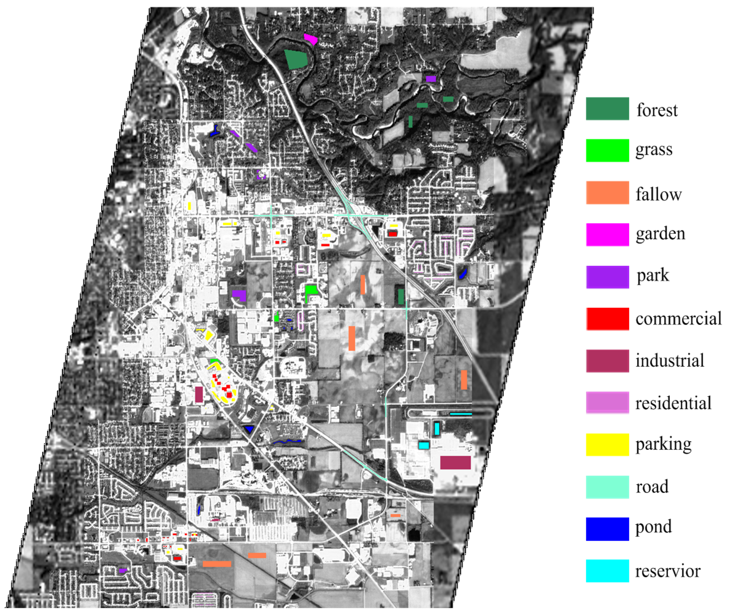
| Class Name | Training Samples | Testing Samples |
|---|---|---|
| forest | 50 | 1688 |
| grass | 50 | 466 |
| fallow | 50 | 1856 |
| garden | 50 | 226 |
| park | 50 | 836 |
| commercial | 50 | 548 |
| industrial | 50 | 1618 |
| residential | 50 | 524 |
| parking | 50 | 918 |
| road | 50 | 1053 |
| pond | 50 | 375 |
| reservoir | 50 | 397 |
| Total | 600 | 10,505 |
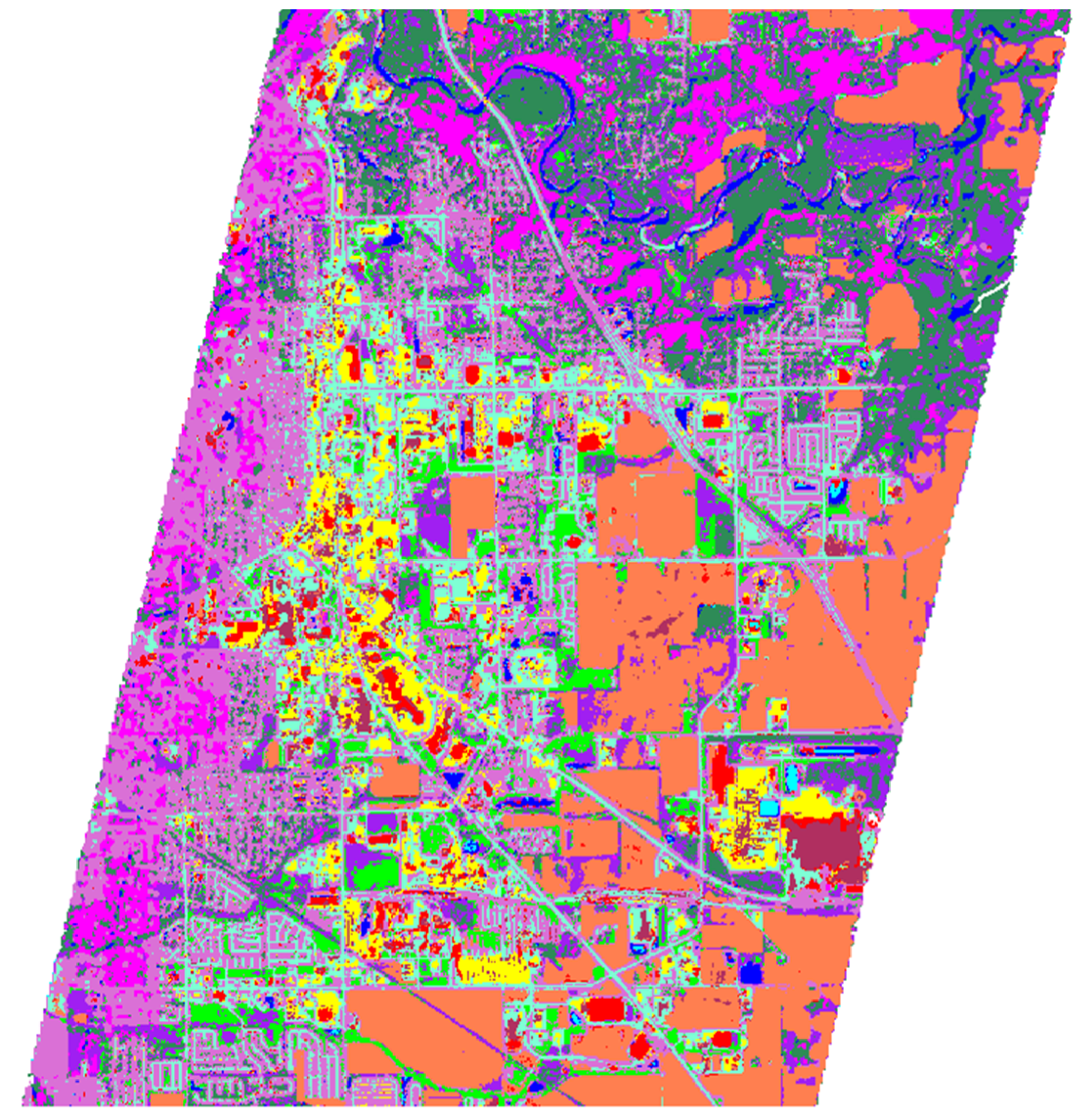
| Classifier | SSR [12] | BayesSR [13] | CNMF [6] | Two-CNN-Fu |
|---|---|---|---|---|
| SVM | 81.53 ± 1.18% | 77.01 ± 0.97% | 86.54 ± 0.98% | 89.81 ± 0.86% |
| CCF | 85.04 ± 0.64% | 80.74 ± 0.73% | 89.75 ± 1.50% | 94.15 ± 0.47% |
| Network Parameter | Indian Pines | Moffett Field | Berlin | |
|---|---|---|---|---|
| Size of conv. kernels in HSI branch | 40 × 1 | 31.7423 | 31.7852 | 30.8647 |
| 45 × 1 | 32.3584 | 32.6985 | 31.3642 | |
| 50 × 1 | 31.0257 | 31.3584 | 31.4375 | |
| Size of conv. kernels in MSI branch | 9 × 9 | 32.3351 | 32.5304 | 30.9785 |
| 10 × 10 | 32.3584 | 32.6985 | 31.3642 | |
| 11 × 11 | 31.6574 | 31.8458 | 30.9775 | |
| Number of kernels per conv. layer in HSI branch | 10 | 31.1474 | 31.2045 | 30.9775 |
| 20 | 32.3584 | 32.6985 | 31.3642 | |
| 30 | 32.1054 | 32.5447 | 31.2875 | |
| Number of kernels per conv. layer in MSI branch | 20 | 32.2446 | 32.1454 | 31.0847 |
| 30 | 32.3584 | 32.6985 | 31.3642 | |
| 40 | 31.7822 | 32.2841 | 31.1765 | |
| Number of neurons per FC layer | 400 | 32.0454 | 32.3747 | 30.8749 |
| 450 | 32.3584 | 32.6985 | 31.3642 | |
| 500 | 32.2042 | 32.4876 | 31.4756 | |
| Size of input patch of MSI branch | 29 × 29 | 31.8624 | 32.3414 | 30.6987 |
| 31 × 31 | 32.3584 | 32.6985 | 31.3642 | |
| 33 × 33 | 31.7457 | 31.9771 | 31.0876 | |
| Number of FC layers | 2 | 31.8634 | 31.7985 | 31.1442 |
| 3 | 32.3584 | 32.6985 | 31.3642 | |
| 4 | 32.2047 | 32.3847 | 31.3970 | |
| Number of conv. layers | 2 | 31.9852 | 32.3247 | 31.1093 |
| 3 | 32.3584 | 32.6985 | 31.3642 | |
| 4 | - | - | 31.2595 |
© 2018 by the authors. Licensee MDPI, Basel, Switzerland. This article is an open access article distributed under the terms and conditions of the Creative Commons Attribution (CC BY) license (http://creativecommons.org/licenses/by/4.0/).
Share and Cite
Yang, J.; Zhao, Y.-Q.; Chan, J.C.-W. Hyperspectral and Multispectral Image Fusion via Deep Two-Branches Convolutional Neural Network. Remote Sens. 2018, 10, 800. https://doi.org/10.3390/rs10050800
Yang J, Zhao Y-Q, Chan JC-W. Hyperspectral and Multispectral Image Fusion via Deep Two-Branches Convolutional Neural Network. Remote Sensing. 2018; 10(5):800. https://doi.org/10.3390/rs10050800
Chicago/Turabian StyleYang, Jingxiang, Yong-Qiang Zhao, and Jonathan Cheung-Wai Chan. 2018. "Hyperspectral and Multispectral Image Fusion via Deep Two-Branches Convolutional Neural Network" Remote Sensing 10, no. 5: 800. https://doi.org/10.3390/rs10050800
APA StyleYang, J., Zhao, Y.-Q., & Chan, J. C.-W. (2018). Hyperspectral and Multispectral Image Fusion via Deep Two-Branches Convolutional Neural Network. Remote Sensing, 10(5), 800. https://doi.org/10.3390/rs10050800