Abstract
Enhancing the spatial resolution of hyperspectral image (HSI) is of significance for applications. Fusing HSI with a high resolution (HR) multispectral image (MSI) is an important technology for HSI enhancement. Inspired by the success of deep learning in image enhancement, in this paper, we propose a HSI-MSI fusion method by designing a deep convolutional neural network (CNN) with two branches which are devoted to features of HSI and MSI. In order to exploit spectral correlation and fuse the MSI, we extract the features from the spectrum of each pixel in low resolution HSI, and its corresponding spatial neighborhood in MSI, with the two CNN branches. The extracted features are then concatenated and fed to fully connected (FC) layers, where the information of HSI and MSI could be fully fused. The output of the FC layers is the spectrum of the expected HR HSI. In the experiment, we evaluate the proposed method on Airborne Visible Infrared Imaging Spectrometer (AVIRIS), and Environmental Mapping and Analysis Program (EnMAP) data. We also apply it to real Hyperion-Sentinel data fusion. The results on the simulated and the real data demonstrate that the proposed method is competitive with other state-of-the-art fusion methods.
PACS:
J0101
1. Introduction
Hyperspectral images (HSIs) contain rich spectral information, which is beneficial for discriminating between different materials in the scene. Due to the discriminative ability, HSI has been applied in many fields, including target detection [1], mineral exploitation [2], and land cover classification [3]. Earth observation applications often need HSI with high spatial resolution. However, the spatial resolution of HSI is often limited because of the trade-off between the spatial and spectral resolution (e.g., Hyperion HSI is of 30 m spatial resolution). Compared with HSIs, multispectral images (MSI) have wider bandwidth, and are often of higher spatial resolution (e.g., ASTER MSI is of 15 m resolution). Fusing low resolution (LR) HSIs with a high resolution (HR) MSIs is an important technology to enhance the spatial resolution of HSI [4,5].
Several HSI-MSI fusion algorithms have been proposed in the last decades [4,5,6,7,8,9,10,11,12,13,14,15,16,17,18,19,20]. HR HSI can be reconstructed by combining endmember of LR HSI and an abundance of HR MSI. According to this principle, several unmixing based fusion methods have been proposed. For example, in [6], HSI and MSI were alternatively unmixed by applying nonnegative matrix factorization in a coupled way; thus, HR HSI was reconstructed with the endmember and the HR abundance under a linear mixture model. This method was also used to fuse Hyperion HSI with ASTER MSI and produce HSI with 15 m resolution [7]. Similarly, by exploiting the sparsity prior of endmembers, a fusion method based on sparse matrix factorization was proposed in [8]. It was also used to fuse MODIS HSI with Landsat 7 ETM + MSI, and to enhance the resolution of MODIS HSI by 8 times [9]. HR HSI can also be reconstructed with a dictionary. In [10,11], a spatial dictionary was learned from HR MSI, and HR HSI was then reconstructed via joint sparse coding. In [12,13], a spectral dictionary was learned from LR HSI, then it was used to reconstruct HR HSI based on the abundance map of MSI. The HSI-MSI fusion problem could also be solved in a variation framework [14,15,16,17]. Wei et al. [14] proposed a variation model for the HSI-MSI fusion whereby the sparsity prior of HSI was exploited as a regularizer. Other than the sparsity regularizer, a vector-total-variation regularizer was used in [15], a low rank constraint and a spectral embedding regularizer were designed for fusion in [16]. In [17], a maximum a posteriori fusion method was proposed by exploiting the joint statistics of endmembers under a stochastic mixing model. A new concept, “hypersharperning”, was proposed in [18], and applied to Worldview-3 data in [19], which aims at fusing LR HSI in the short-wavelength infrared bands with HR HSI in the visible and near infrared bands of the same sensor.
Most of the above fusion methods suffer from three major drawbacks. Firstly, they are based on hand-crafted features such as the dictionary, which can be regarded as low-level feature with limited representative ability. Secondly, they rely on prior assumptions, such as the linear spectral mixture assumption in [6,7,8,9], and the sparsity prior in [10,11,12,13,14]. Quality degeneration may be caused if these assumptions do not fit the problem. Finally, optimization problems are often involved in the testing stage, making the HSI reconstruction time-consuming. Recently, deep learning has attracted research interests due to its ability to automatically learn high-level features, and its high non-linearity [21,22,23,24,25,26,27,28], which is of great potential for modeling the complex nonlinear relationship between LR and HR HSIs in both the spatial and spectral domains. Compared with the hand-crafted features, the features extracted by deep learning are hierarchical: both of the low-level and high-level features can be extracted, which would be more comprehensive and robust for reconstructing HR HSI. In addition, deep learning is data-driven; it does not rely on any assumption or prior knowledge. After the off-line training, only feed forward computation is needed in the testing stage of deep learning, which would make the HSI reconstruction fast. Therefore, the performance is expected to be improved if deep learning is applied to the spatial enhancement of HSI.
Among the typical deep learning models, convolutional neural networks (CNN) are the most widely used model for single image enhancement. Several CNN-based image super-resolution methods has been proposed [29,30,31,32,33]. The success of CNN in image super-resolution could be summarized by the following three points. Firstly, CNN is built upon 2-D convolution computation, which could naturally exploit the spatial correlation of images. Secondly, CNN with deep architecture has large capacity and flexibility for representing the mapping between LR and HR images [34]. Thirdly, compared with other deep learning models, such as stacked auto-encoders (SAE) [35], due to the weight sharing and local connection scheme, CNN often has fewer connections, and is less prone to over-fitting [36].
Inspired by the success of CNN in single image enhancement, in this study, we propose a deep CNN with a two-branch architecture for the fusion of HSI and MSI. In order to exploit the spectral correlation of HSI and fuse the MSI, the spectrum of LR HSI and the corresponding spatial neighborhood in HR MSI is used as input pair of the network. We extract the features from the spectrum of LR HSI and the corresponding neighborhood in MSI with the two CNN branches. In order to fully fuse the information extracted from HSI and MSI, the extracted features of the two branches are concatenated and then fed to fully connected (FC) layers. The final output of the FC layers is the spectrum of the expected HR HSI.
We consider three main contributions in this work:
- We propose learning the mapping between LR and HR HSIs via deep learning, which is of high learning capacity, and is suitable to model the complex relationship between LR and HR HSIs.
- We design a CNN with two branches extracting the features in HSI and MSI. This network could exploit the spectral correlation of HSI and fuse the information in MSI.
- Instead of reconstructing HSI in band-by-band fashion, all of the bands are reconstructed jointly, which is beneficial for reducing spectral distortion.
The rest of this paper is organized as follows. In Section 2, some basics on deep learning-based image super-resolution are presented. In Section 3, we give the proposed HSI-MSI fusion method based on deep learning, including the architecture of the network and the training scheme. Experiment results on the simulated and real HSI are presented in Section 4. Discussions on the experiment results are in Section 5. We make the conclusions in Section 6.
2. Background of CNN Based Image Super-Resolution
CNN has been successfully applied to spatial enhancement of single images [29,30,31,32,33]. In [29], Dong et al. proposed a super-resolution CNN network (SRCNN). As shown in Figure 1, the CNN architecture for super-resolution is composed of several convolutional layers. The input of the network is the LR image, which is first up-scaled to the same size of its HR version. Activity of the i-th feature map in the l-th convolutional layer can be expressed as [36]
where is the j-th feature map in the (l − 1)-th layer that connected to in the l-th convolutional layer. , are the number of rows and columns of . is the convolutional kernel for associated with the i-th output feature , and is the size of the kernel. is bias. denotes the convolutional operator. The size of is . is a nonlinear activation function, such as rectified linear units (ReLU) function [36]. The output of the network is the expected HR image. In the training stage, the mapping function between the up-scaled LR and HR images can be learned and represented by the CNN network. In the testing stage, the HR image is reconstructed from its LR counterpart with the learned mapping function.
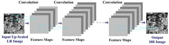
Figure 1.
A typical CNN architecture for super-resolution of single image.
Inspired by this idea, some other CNN based super-resolution methods have also been proposed. For example, a faster SRCNN (FSRCNN) was proposed by adopting a deconvolution layer and small kernel size in [30]. Kim et al. [31] pointed out that increasing the depth of CNN is helpful for improving the super-resolution performance. A very deep CNN for super-resolution (VDSR) was proposed and trained with a residual learning strategy in [31]. In [32], the authors proposed an end-to-end deep and shallow network (EEDS) composed of a shallow CNN and a deep CNN, which restored the principle component and the high-frequency component of the image respectively. In order to reduce the difficulty of enhancing the resolution by a large factor, the authors in [33] proposed a gradual up-sampling network (GUN) composed of several CNN modules, in which each CNN module enhanced the resolution by a small factor.
Other than single image super-resolution, CNN also shows the potential in HSI super-resolution. The mapping between LR and HR HSIs can be learned for super-resolution by different deep learning models, such as 3D-CNN [37]. A deep residual CNN network (DRCNN) with spectral regularizer was proposed for HSI super-resolution in [38]. In [39], a spectral difference CNN (SDCNN) was proposed, which learns the mapping of spectral difference between LR and HR HSIs. CNN has also been applied to pan-sharpening. In [40], HR panchromatic image was stacked with up-scaled LR MSI to form an input cube, a pan-sharpening CNN network (PNN) was used to learn the mapping between the input cube and HR MSI. A deep residual PNN (DRPNN) model was proposed to boost PNN by using residual learning in [41]. In [42], in order to preserve image structures, the mapping was learned by a residual network called PanNet in the high-pass filtering domain, rather than the image domain. Multi-scale information could be exploited in mapping learning. In [43], Yuan et al. proposed a multi-scale and multi-depth CNN (MSDCNN) for pan-sharpening, whereby each layer was constituted by filters with different sizes for the multi-scale features.
The above CNN-based super-resolution methods are also summarized in Table 1. Despite the success of CNN in super-resolution and pan-sharpening, two issues still exist when applying deep learning to HSI super-resolution. On the one hand, the CNN models for single image super-resolution mainly deal with the spatial domain, while for HSI, the deep learning model should also exploit the spectral correlation of HSI, and jointly reconstruct different bands. On the other hand, some auxiliary data (e.g., MSI) of the same scene with HSI is often available; these auxiliary data can provide complementary information for HSI super-resolution. The means to fuse HSI with these auxiliary data in the deep learning framework still lacks study.

Table 1.
A summary of CNN based image super-resolution methods.
3. HSI and MSI Fusion Based on Two-Branches CNN
3.1. The Proposed Scheme of Deep Learning Based Fusion
The previous deep learning-based single image super-resolution methods learn the mapping between LR and HR images in the spatial domain. In this study, we propose learning the mapping between LR and HR HSIs in the spectral domain, where the relationship between LR and HR HSIs is similar to that of the spatial domain. We give an example in Figure 2. The left image in Figure 2a is an original HR image cropped from AVIRIS Indian pine data. The right image in Figure 2a is a simulated LR image, which is firstly down-sampled from the HR HSI by a factor of two, and then up-scaled to the same size of the HR HSI. In Figure 2, it can be seen that the LR image is highly correlated with its HR version, but that the LR image is blurred, and that some high-frequency component is missed in the LR image. In Figure 2b, we select two different land-covers and give their spectra. It is clear that the spectrum in the LR HSI is also highly correlated with its counterpart in the HR HSI, and some high-frequency component in the spectrum of LR HSI is missed, as shown in Figure 2b.
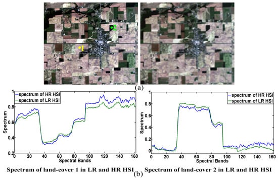
Figure 2.
(a) Color composite (bands 29, 16, 8) of HR HSI (left) and LR HSI (right), the image is cropped from AVIRIS Indian pines data; (b) Spectra of two different land-covers in HR HSI and LR HSI, the two land-covers are marked in (a).
Therefore, the mapping between LR and HR HSIs in the spectral domain has a similar pattern to that of the spatial domain. Instead of learning the mapping in the spatial domain, in this study, we learn the mapping between the spectra of LR and HR HSIs. Three advantages are considered here. Firstly, the deep learning network extracts features from the spectrum of LR HSI, the spectral correlation of HSI could be exploited by deep learning. Secondly, the deep learning network would output the spectrum of the expected HR HSI, so all of the bands of HR HSI could be jointly reconstructed, which is beneficial for reducing the spectral distortion. Thirdly, we propose to extract features from the spectrum of LR HSI. Compared with extracting features from a 3D HSI block, this involves less computation and lower network complexity.
We propose a framework of deep learning based HSI-MSI fusion in Figure 3. A deep learning network is used to model the mapping between the spectra of LR and HR HSIs. In order to fuse MSIs, we should also extract the features from the MSIs with the deep learning model. The features extracted from the HSI and MSI would be fused by the deep learning network. After learning the mapping function, the deep learning model could reconstruct the spectrum of the HR HSI.
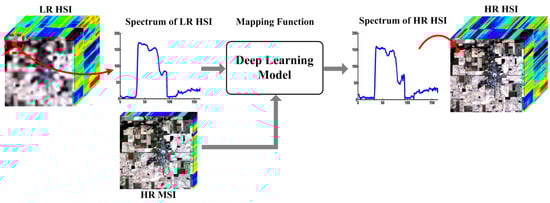
Figure 3.
The proposed scheme of deep learning based HSI-MSI fusion.
3.2. Architecture of the Two Branches CNN for Fusion
According to the framework in Figure 3, we design a CNN model with a two-branch architecture for HSI-MSI fusion, as shown in Figure 4. The two CNN branches are devoted to extracting the features from the LR HSI and the HR MSI. The LR HSI is firstly up-scaled to the same size with the HR MSI, features are extracted by the two branches from the spectrum of each pixel in the up-scaled HSI, and its corresponding spatial neighborhood in the HR MSI. The HSI branch takes spectrum of the n-th pixel in the up-scaled HSI as input, after l layers of convolutional operation in Equation (1), we could extract features from the LR HSI. It should be noted that the input is a 1-D signal. Therefore, all of the convolutional operations in this branch reduce to 1-D computation, so all of the convolutional kernels and feature maps per convolutional layer in this branch reduce to 1-D case.
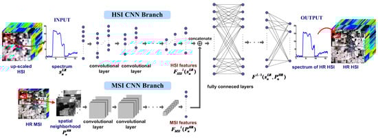
Figure 4.
The proposed two branches CNN architecture for HSI-MSI fusion.
In order to fuse the spatial information in the MSI of the same scene, the corresponding spatial neighboring block in the MSI (as shown in the red box in Figure 4) of the n-th pixel is used as input for the MSI branch, where r is block size (it is fixed to 31 × 31 in the experiment), and b is the number of bands of MSI. All bands in MSI are used for fusion in this branch. After l convolutional layers in this branch, we can extract features from the MSI.
It is noted that and are obtained by vectorizing the feature maps of the HSI and MSI branches respectively. In order to fuse the information of HSI and MSI, we concatenate the extracted features and , then simultaneously feed them to the FC layers. The output of the (l + 1)-th layer is
where and are the weight matrix and the bias of the FC layer, respectively. means concatenating the HSI features and the MSI features. FC layers are adopted here because they could fully fuse the information of HSI and MSI. After several FC layers, the output of the last FC layer is the reconstructed spectrum of the expected HR HIS
where and are the weight matrix and the bias of the L-th FC layer, respectively. is the feature vector of the (L − 1)-th FC layer. All the convolutional kernels, weight matrices and bias values in the network are trained in an end-to-end fashion. In the testing stage, we extracted the spectrum of the up-scaled HSI from each pixel and its corresponding neighborhood block in the HR MSI, then fed them to the trained network. The output of the network is the spectrum of the expected HR HSI. After putting back the reconstructed spectrum to each pixel, a HR HSI could be obtained.
In the training stage, the LR HSI is firstly up-scaled to the same size of the HR MSI. Although the up-scaled HSI has the same size with the HR HSI, it is still blurring, as shown in Figure 4. The purpose of up-scaling is to match the size of LR HSI to that of HR MSI and HR HSI. This strategy has also been adopted in other deep learning-based image super-resolution methods, for example, in [29,30,34]. The deep learning model is trained to learn the mapping between up-scaled HSI and HR HSI. In the testing stage, we should also firstly up-scale the LR HSI to the size of the HR HSI using the same interpolation algorithm as the training stage, then feed it to the trained deep learning network. In this way, an HR HSI with better quality could be recovered.
3.3. Training of the Two Branches CNN
All the convolutional kernels, weight matrices, and bias values in the network are trained by minimizing the reconstruction error of the HR HSI spectra. The Frobenius norm is used to measure the reconstruction error in the loss function. The set of training samples is denoted as , and the loss function is written as
where N is number of training samples. For the n-th training sample, is the spectrum of LR HSI, is the corresponding spatial neighborhood in HR MSI, and is the spectrum of HR HSI. is the reconstructed spectrum of HR HSI. The loss function is optimized using the stochastic gradient descent (SGD) method with standard back-propagation [44].
4. Experiment Results
In this section, the performance of the proposed fusion algorithm (denoted as Two-CNN-Fu) is evaluated on several simulated and real HSI datasets. We first evaluate the proposed method on the simulated data by comparing it with other state-of-the-art fusion methods. In order to demonstrate the applicability of the proposed method, we also apply it on real spaceborne HSI-MSI fusion. Because the original HR HSI is not available in this case, and there is no reference HSI for assessment, we use our previously proposed no-reference HSI quality assessment method in [45] to evaluate the fusion performance; land-cover classification accuracy of the fused HSI is also used to evaluate the fusion performance.
4.1. Experiment Setting
Two datasets are used in the experiment. The first dataset was collected by an Airborne Visible Infrared Imaging Spectrometer (AVIRIS) sensor [46], which consists of four images captured over Indian Pines, Moffett Field, Cuprite, and Lunar Lake sites with dimensions 753 × 1923, 614 × 2207, 781 × 6955 and 614 × 1087, respectively. The spatial resolution is 20 m. The dataset was taken in the range of 400~2500 nm, with 224 bands. After discarding the water absorption bands and noisy bands, 162 bands remained. The second one is Environmental Mapping and Analysis Program (EnMAP) data, which was acquired by HyMap sensor over Berlin district on August 2009 [47,48]. The size of this data is 817 × 220 with spatial resolution 30 m. There are 244 spectral bands in the range of 420~2450 nm.
Higher resolution MSIs as relative to future earth observation hyperspectral sensors are available. But due to the fact that earth observation HSIs with reference (at higher spatial resolution for evaluation) are not available, simulations are often used. The above HSI datasets are regarded as HR HSI and reference image, and both LR HSI and HR MSI are simulated from them. The LR HSI are generated from the reference image via spatial Gaussian down-sampling. The HR MSI is obtained by spectrally degrading the reference image with the spectral response function of Landsat-7 multispectral imaging sensor as filters. There are six spectral bands of the simulated MSI, which cover the spectral regions of 450~520 nm, 520~600 nm, 630~690 nm, 770~900 nm, 1550~1750 nm, and 2090~2350 nm, respectively. We crop two sub-images of 256 × 256 from Indian pines and Moffett Field from the AVIRIS dataset, and one sub-image of 256 × 160 from Berlin from the EnMAP dataset as testing data. Fifty thousand samples are extracted for training each Two-CNN-Fu model. There is no overlapping between the testing region and the training region. The network is trained on the down-sampled data; the original HR HSI does not appear in training, and is only used as an assessment reference.
The network parameters of our deep learning model are given in Table 2. The deep learning network needs to be initialized before the training. All of the convolutional kernels and weight matrix of the FC layers are initialized from Gaussian random distribution, with standard variance of 0.01 and a mean 0. The bias values are initialized to 0. The parameters involved in the standard stochastic gradient descent method are learning rate, momentum, and batch size [44]. The learning rate is fixed at 0.0001, momentum is set to 0.9, and the batch size is set to 128. The number of training epochs is set to 200.
Table 2.
The parameter setting of the network architecture.
4.2. Comparison With State-of-the-Art Methods
In this section, we compare our method with other state-of-the-art fusion methods. The compared methods are: the coupled nonnegative matrix factorization (CNMF) method [6], the sparse spatial-spectral representation method (SSR) [12], and the Bayesian sparse representation method (BayesSR) [13]. The Matlab codes of these methods are released by the original authors. The parameter settings in the compared methods first follow the suggestions from the original authors; we then empirically tune them, to achieve the best performance. The number of endmembers is a key parameter for the CNMF method; it is set to 30 in the experiment. The parameters in the SSR method include the number of dictionary atoms, the number of atoms in each iterations, and the spatial patch size, which are set to 300, 20, and 8 × 8, respectively. The parameters in the BayesSR method consist of the number of inferencing sparse coding in Gibbs sampling process, and the number of iterations of dictionary learning, which are set to 32 and 50,000, respectively. It is noted that all the compared methods fuse LR HSI with HR MSI. Although there are some deep learning-based HSI super-resolution methods, such as 3D-CNN [37], only LR HSI was exploited in these methods. Therefore, they are not used for comparison for reasons of fairness.
The fusion performance is evaluated by peak-signal-noise-ratio (PSNR, dB), structural similarity index measurement (SSIM) [49], feature similarity index measurement (FSIM) [50], and spectral angle mean (SAM). We calculate PSNR, SSIM, and FSIM on each band, and then compute the mean values over the bands. The indices on the three testing data are given in Table 3 and Table 4. The best indices values are highlighted in bold.
Table 3.
The evaluation indices of different fusion methods on the three testing data by a factor of two.
Table 4.
The evaluation indices of different fusion methods on the three testing data by a factor of four.
It can be seen that our proposed Two-CNN-Fu method has competitive performance on the three testing data. In Table 3, the PSNR, SSIM, and FSIM of our results are higher than those of compared methods, which means that our fusion results are closer to the original HR his, with fewer errors. The SSR method is based on spatial-spectral sparse representation; a spectral dictionary is first learned with the sparsity, and then combined with the abundance of MSI to reconstruct the HR HSI. While in the CNMF method, the endmember of LR HSI and the abundance of MSI are alternatively estimated in a coupled way, the estimated endmember and the abundance would be more accurate, so CNMF could achieve better performance than SSR. The BayesSR method learns the dictionary in a non-parametric Bayesian sparse coding framework, and often performs better than the parametric SSR method. The best performance is achieved by Two-CNN-Fu on the three testing data. Two-CNN-Fu extracts hierarchical features, which are more comprehensive and robust than the hand-crafted features in [6,12,13]. The performance of Two-CNN-Fu demonstrates the effectiveness and potential of deep learning in the HSI-MSI fusion task. In order to verify the robustness over a larger resolution ratio between LR HSI and HR MSI, we also simulate the LR HSI by a factor of four, and then fuse it with MSI. The Two-CNN-Fu also performs better than other methods, as shown in Table 4. The PSNR curves over the spectral bands are presented in Figure 5. It can be found that the PSNR values of Two-CNN-Fu are higher than compared methods in most bands.
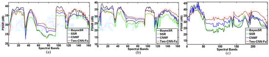
Figure 5.
PSNR values of each band of different fusion results by a factor of two, (a) on AVIRIS Indian pines data; (b) on AVIRIS Moffett Field data; (c) on EnMAP Berlin data.
It is worth noting that the result of our Two-CNN-Fu method has the lowest spectral distortion among the compared methods in most cases, as shown in Table 3 and Table 4. Our deep learning network directly learns the mapping between the spectra of LR and HR HSIs. The objective function Equation (4) for training the network aims at minimizing the error of the reconstructed spectra of HR HSI. In addition, instead of reconstructing HSI in a band-by-band way, our deep learning model jointly reconstructs all bands of HSI. These two characteristics are beneficial for reducing the spectral distortion.
We present parts of the reconstructed HSIs in Figure 6, Figure 7 and Figure 8. In order to visually evaluate the quality of different fusion results, we also give pixel-wise root mean square error (RMSE) maps, which reflect the errors of reconstructed pixels over the whole bands. It is clear that the fusion result of our Two-CNN-Fu method has fewer errors than the compared methods. The compared methods rely on hand-crafted features such as the dictionary. Their RMSE maps have materials-related patterns, which may be caused by the errors introduced in dictionary learning or endmember extraction. Our Two-CNN-Fu method reconstructs the HR HSI based on the mapping function between LR and HR HSIs, which is trained by minimizing the error of the reconstructed HR HSI, so the fusion result of Two-CNN-Fu has fewer errors.
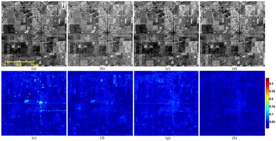
Figure 6.
Reconstructed images (band 70) and root mean square error (RMSE) maps of different fusion results by a factor of four. The testing image is cropped from Indian pines of AVIRIS data with size 256 × 256. (a) result of SSR [12]; (b) result of BayesSR [13]; (c) result of CNMF [6]; (d) result of Two-CNN-Fu; (e) RMSE map of SSR [12]; (f) RMSE map of BayesSR [13]; (g) RMSE map of CNMF [6]; (h) RMSE map of Two-CNN-Fu.
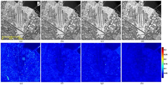
Figure 7.
Reconstructed image (band 80) and root mean square error (RMSE) maps of different fusion results by a factor of two. The testing image is cropped from Moffett Field of AVIRIS data with size 256 × 256. (a) result of SSR [12]; (b) result of BayesSR [13]; (c) result of CNMF [6]; (d) result of Two-CNN-Fu; (e) RMSE map of SSR [12]; (f) RMSE map of BayesSR [13]; (g) RMSE map of CNMF [6]; (h) RMSE map of Two-CNN-Fu.
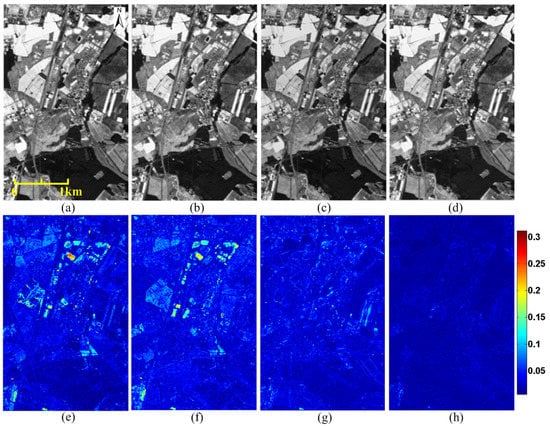
Figure 8.
Reconstructed image (band 200) and root mean square error (RMSE) maps of different fusion results by a factor of two. The testing image is cropped from Berlin of EnMAP data with size 256 × 160. (a) result of SSR [12]; (b) result of BayesSR [13]; (c) result of CNMF [6]; (d) result of Two-CNN-Fu; (e) RMSE map of SSR [12]; (f) RMSE map of BayesSR [13]; (g) RMSE map of CNMF [6]; (h) RMSE map of Two-CNN-Fu.
4.3. Applications on Real Data Fusion
In order to investigate the applicability of the proposed method, we apply the proposed method to real spaceborne HSI-MSI data fusion. The HSI data was collected by Hyperion sensor, which is carried on Earth Observing-1 (EO-1) satellite. This satellite was launched in November 2000. The MSI data was captured by the Sentinel-2A satellite, launched on June 2015. The spatial resolution of Hyperion HSI is 30 m. There are 242 spectral bands in the spectral range of 400~2500 nm. The Hyperion HSI suffers from noise; after removing the noisy bands and water absorption bands, 83 bands remained. The Sentinel-2A satellite provides MSIs with 13 bands. We select four bands with 10 m spatial resolution for the fusion. The central wavelengths of these four bands are 490 nm, 560 nm, 665 nm, and 842 nm, and their bandwidths are 65 nm, 35 nm, 30 nm, and 115 nm, respectively.
The Hyperion HSI and the Sentinel-2A MSI in this experiment were taken over Lafayette, LA, USA in October and November, 2015, respectively [51]. We crop sub-images to 341 × 365 and 1023 × 1095 as study areas from the overlapped region of the Hyperion and Sentinel data, as shown in Figure 9. The remainder of the overlapped region is used for training the Two-CNN-Fu network.
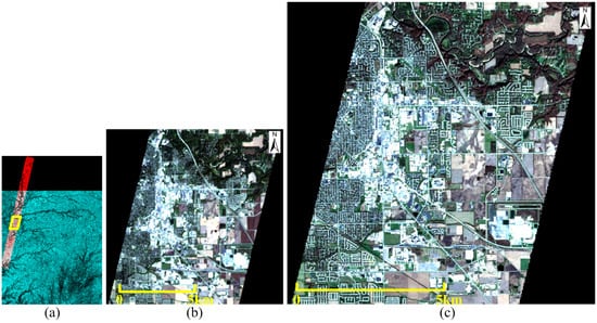
Figure 9.
The experiment data taken over Lafayette, (a) illustration of Hyperion and Sentinel-2A data, the red part is Hyperion data, the green part is Sentinel-2A data, the white part is the overlapped region, the yellow line indicates the study area; (b) color composite (bands 31, 21, 14) of Hyperion data in the study area with size 341 × 365; (c) color composite (bands 4, 3, 2) of Sentinel-2A data in the study area with size 1023 × 1095.
In this experiment, our goal is to fuse the 30 m HSI with the 10 m MSI, and then generate a 10 m HSI, so a Two-CNN-Fu network that could enhance HSI by a factor of three should be trained. In the training stage, we first down-sample the 30 m Hyperion HSI and 10 m Sentinel-2A MSI into 90 m and 30 m, by a factor of three, respectively. Then we train a Two-CNN-Fu network that could fuse the 90 m HSI with the 30 m MSI, and reconstruct the original 30 m HSI. This network could enhance HSI by a factor of three. We assume that it could be transferred to the fusion task of 30 m HSI and 10 m MSI. By applying the trained network to the 30 m HSI and the 10 m MSI, an HSI with 10 m resolution could be reconstructed. The network parameters are set according to Table 2, except that the number of convolutional layers in the HSI branch is one, because we only use 83 bands of the Hyperion data. The maximal number of convolutional layers in the HSI branch is one, in this case.
The fusion results of different methods on the study area are presented in Figure 10. The size of the fusion result is 1023 × 1095. In order to highlight the details of the fusion results, we also display two small areas by enlarging them in Figure 11 and Figure 12. It is clear that there is some noise in the results of SSR and CNMF, as shown in Figure 11b,d. In Figure 12, we also find that some details in the results of SSR and CNMF are blurred, as indicated in the dashed box. The results of BayesSR and Two-CNN-Fu are sharper and cleaner, and our Two-CNN-Fu method produces the HR HSI with higher spectral fidelity. It is clear that the spectral distortion of BayesSR is heavier than our Two-CNN-Fu results, if we compare them with the original LR images. The color of the BayesSR results seems to be darker than the original LR image. Spectral distortion in the fusion would affect the accuracy of applications such as classification.
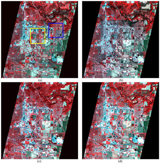
Figure 10.
False color composite (bands 45, 21, 14) of different Hyperion-Sentinel fusion results, size of the enhanced image is 1023 × 1095 with 10 m resolution, (a) result of SSR [12]; (b) result of BayesSR [13]; (c) result of CNMF [6]; (d) result of Two-CNN-Fu.
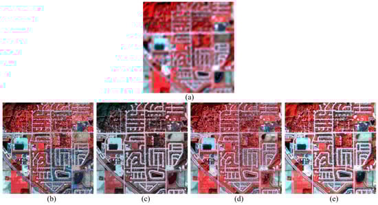
Figure 11.
False color composite (bands 45, 21, 14) of the enlarged area in the blue box of Figure 10, size of the area is 200 × 200, (a) the original 30 m Hyperion data; (b) fusion result of SSR [12]; (c) fusion result of BayesSR [13]; (d) fusion result of CNMF [6]; (e) fusion result of Two-CNN-Fu.
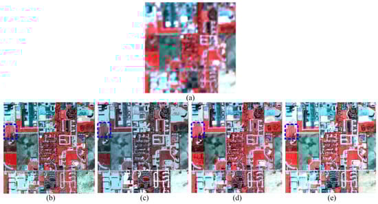
Figure 12.
False color composite (bands 45, 21, 14) of the enlarged area in the yellow box of Figure 10, size of the area is 200 × 200, (a) the original 30 m Hyperion data; (b) fusion result of SSR [12]; (c) fusion result of BayesSR [13]; (d) fusion result of CNMF [6]; (e) fusion result of Two-CNN-Fu.
It is noted that the Hyperion HSI and the Sentinel-2A MSI in this experiment were not captured at the same time; the temporal difference is about one month. Some endmembers may change during this month, which may be one of the factors that lead to the spectral distortion. Even though nearly all of the fusion results in Figure 11 and Figure 12 suffer from the spectral distortion, our Two-CNN-Fu method generates results with less spectral distortion, which demonstrates the robustness of the proposed method.
In order to assess the performance quantitatively, we evaluate the fusion results using the no-reference HSI quality assessment method in [45], which would give quality scores for each reconstructed HSI. In this no-reference assessment method, some pristine HSIs are needed as training data to learn the benchmark quality-sensitive features. We use the original LR Hyperion data after discarding the noisy bands as training data. The quality score measures the distance of the reconstructed HSI and the pristine benchmark; a lower score value means better quality. The quality scores of different fusion results are given in Table 5. The best index is highlighted in bold. It is clear that the score of our fusion result is lower than others. This means that our method is competitive with other compared methods. The larger score values of the compared methods may be caused by the spectral distortion, or the noise in the fusion results.
Table 5.
The no-reference quality assessment scores of different results on Hyperion-Sentinel fusion.
Land-cover classification is one of the important applications of HSI. In this experiment, we test the effect of different fusion methods on the land-cover classification. Land-cover information is provided by Open Street Map (OSM) layers [52]. According to the OSM data, there are 12 classes of land-covers in the study area. We select parts of the pixels from each class as ground truth, as shown in Figure 13 and Table 6. Two classifiers, Support Vector Machine (SVM) [53] and Canonical Correlation Forests (CCF) [54], are used in the experiment due to their stability and good performance. The SVM classifier is implemented with the LIBSVM toolbox [55], and the radial basis function is used as kernel function of SVM. The regularization parameters in SVM are determined by five-fold cross-validation in the range of . The parameter involved in the CCF classifier is the number of trees; we set it to 200 in the experiment. Fifty samples of each class are randomly chosen for training the classifiers; the remainder of the ground truth are used as testing samples. We repeat the classification experiment 10 times, and then report the mean value and standard variance of overall accuracy in Table 7. The best indices are highlighted in bold.
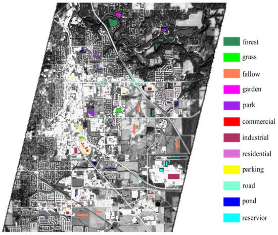
Figure 13.
The ground truth labeled from each class.
Table 6.
The number of ground truth labeled in the study area.
Table 7.
The Overall Accuracy (OA) of different fusion results.
In Table 7, it can be found that our fusion result can lead to competitive classification accuracy on both SVM and CCF classifiers, and the classification results have similar trend on the two classifiers. The classification accuracy of our fusion result is higher than that of the other three fusion methods. As we can observe in Figure 11 and Figure 12, the spectral distortion and noise of our fusion method is less than that of other methods, which may explain why our classification accuracy is higher. The classification map of Two-CNN-Fu fusion results is given in Figure 14. In Figure 14, most of the land-covers can be classified correctly; even some details, such as roads and residential areas can be classified well with the fusion enhanced image. Misclassification of some land-covers, such as forests and gardens, may be caused by the similarity in spectra between these two land-covers. It is worth noting that the fusion method can not be absolutely assessed by the classification accuracy, because our labeled ground truth is only a subset of the study area, and the classification performance also depends on the classifier. The aim of this classification experiment is to demonstrate that our proposed fusion method has the potential to be applied in real spaceborne HSI-MSI fusion, and the reconstructed HR HSI could result in competitive classification performance.
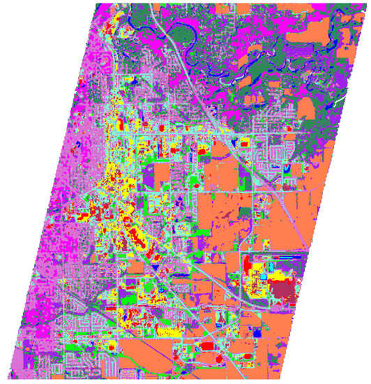
Figure 14.
The classification map of Hyperion-Sentinel fusion result by Two-CNN-Fu method, the classifier is CCF.
5. Some Analysis and Discussions
5.1. Sensitivity Analysis of Network Parameters
The architecture parameters of the deep learning model need to be tuned to achieve satisfactory performance. It is theoretically hard to determine the optimal combination of these parameters. We empirically tune the architecture parameters of Two-CNN-Fu, which are given in Table 2. In this sub-section, sensitivity analysis of Two-CNN-Fu over these parameters is presented. We vary one architecture parameter and fix others, then observe the corresponding fusion performance on a validation set, which consists of 50 randomly selected patches of size 64 × 64. It is noted that there is no overlapping among the training set, the validation set, and the testing images. The PSNR indices of the sensitivity analysis over the network parameter are given in Table 8. The best indices are highlighted in bold.
Table 8.
PSNR (dB) indices of the sensitivity analysis over the network parameters.
The size of convolutional kernel should be large enough to collect enough information from the spectrum of HSI and the corresponding spatial neighborhood of MSI. As shown in Table 8, it can be found that the kernel size of 45 × 1 in the HSI branch and 10 × 10 in the MSI branch could lead to the best results in most cases. It is noted that such kernel size would not result in the best performance on EnMAP Berlin. However, the extent of performance decrease is not significant, so we fix the kernel size to 45 × 1 in the HSI branch and 10 × 10 in the MSI branch in the experiment.
The number of kernels per convolutional layer is also an important parameter. In Table 8, the best performance is obtained when we set 20 convolutional kernels per layer in the HSI branch, and 30 convolutional kernels per layer in the MSI branch. If the number of kernels is smaller, the deep learning network can not extract enough features for the fusion. With the increase of kernel number, the network would become more complex, and more parameters need to be trained, and more training data is required. This may explain the performance drop with the increased number of kernels.
Higher level features that contain information about the HSI and MSI would be learned by the FC layers. The size of the learned features is determined by the number of neurons per FC layer. If the size is too small, the capacity of the network would be limited. In our experiment, the best result is achieved when the number of neurons is set to 450 per FC layer in most cases. When the number of neurons increases, the performance declines.
The number of layers is an important parameter for deep learning model. With more layers, the deep learning network would have a higher capacity, and could learn mapping functions that are more complex. It is noted that the number of bands of AVIRIS Moffett Field and Indian pines data is 162, and the maximal number of convolutional layers we can set is three, according to the architecture in Table 2. In Table 8, it is clear that the best results can be obtained with three convolutional layers and three FC layers in most cases. Therefore, we set three convolutional layers and three FC layers in our final network.
The sensitivity over the MSI patch size is also given in Table 8. It is worth noting that the network parameters in Table 2 are selected with the fixed MSI patch size 31 × 31; this combination leads to the best result in most cases. Therefore, an MSI patch that is smaller or bigger would result in a reduced performance if we set the network parameters according to Table 2.
The evolution of loss function values during the training are presented in Figure 15. The loss function declines drastically in the first 20 epochs, then tends to be a constant after the big descent. The loss function would decrease by a small margin after 160 epochs. Therefore, we set the number of epochs to 200, which is adequate to converge to a local minimum and generate a satisfactory result.
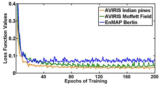
Figure 15.
Evolution of loss function value over epochs of training.
5.2. Robustness Analysis over Training Data
In the previous sections, we trained the Two-CNN-Fu network and tested the performance on data collected by the same sensor. In this section, we investigate the robustness of the Two-CNN-Fu network over the training data. We train the network on AVIRIS data and test the performance on EnMAP Berlin data by transferring the pre-trained network to EnMAP Berlin data. Since the two sensors have different numbers of spectral bands, the weight matrices of the first and the last FC layers need to be fine-tuned on EnMAP data. Other layers of the pre-trained network could be transferred and utilized directly. The evolution of the fusion performance over the epochs of fine-tuning is given in Figure 16. It is clear that the fusion performance can approximate or even surpass the original network trained on EnMAP data after only a few epochs of fine-tuning.

Figure 16.
Evolution of fusion performance over epochs of fine-tuning, the testing data is EnMAP Berlin data, (a) the first and last FC layers are fine-tuned on EnMAP; (b) all of the three FC layers are fine-tuned on EnMAP.
Although there is considerable difference in the spectral configurations of AVIRIS and EnMAP data, the network trained on AVIRIS data can be generalized to EnMAP data after fine-tuning. This can be explained by the hierarchy of deep learning. The bottom layers capture low-level features, such as edges and corners. These features are generic, and could be transferred to different data or sensors. The top layers extract features that are specific to the data, which need to be fine-tuned [56,57]. Therefore, when we apply Two-CNN-Fu to new data. Instead of training a whole network from scratch, we could transfer a pre-trained network to the new data and fine-tune the FC layers with only a few epochs. Satisfactory performance is expected to be achieved in this way.
5.3. Visualization of the Extracted Features
To better understand the features extracted by the network, parts of the learned kernels and the extracted features are visualized in this sub-section. In Figure 17, we show parts of the convolutional kernels in the MSI branch trained on EnMAP Berlin data. It can be observed that the convolutional kernels in different layers reveal different patterns. For example, in Figure 17a, the first kernel in the first row looks like Gaussian filter, whereas the first two kernels in the second row are like Laplacian filters, which would extract high-frequency information, such as edges and textures. In Figure 17b,c, the kernels in the second and third convolutional layers also reveal some patterns, but these kernels are more abstract than those of the first layer.
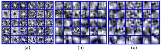
Figure 17.
The kernels of different convolutional layers in MSI branch trained on EnMAP Berlin data, (a) kernels of the first layer; (b) kernels of the second layer; (c) kernels of the third layer.
In Figure 18, we present parts of the feature maps in the MSI branch. The input MSI is simulated from EnMAP Berlin data with size 128 × 128. As shown in the first three maps in Figure 18b, some high-frequency features, such as the textures and edges in different orientations, could be extracted in the first convolutional layer. This observation is also consistent with the patterns revealed by the convolutional kernels in Figure 17a. Compared with the first convolutional layer, the feature maps in the second and third convolutional layers are more abstract.
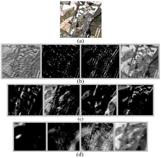
Figure 18.
The extracted feature maps of different convolutional layers in MSI branch, the features are extracted from simulated MSI with size 128 × 128, the data is simulated from EnMAP Berlin data, (a) input MSI data; (b) feature maps of the first layer; (c) feature maps of the second layer; (d) feature maps of the third layer.
We also give parts of the features extracted by different convolutional layers in the HSI branch in Figure 19. The features are extracted from the spectrum located at (76,185) of the AVIRIS Indian pines data. As shown in Figure 19a, the features extracted by the first convolutional layer in the HSI branch are concerned with the shape and the high-frequency components. Similar to the MSI branch, the features in the higher layers are more abstract than those of the first layer. Different layers extract features from different perspectives; all these features would make contributions to the HSI and MSI fusion task.
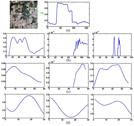
Figure 19.
The extracted features of different convolutional layers in HSI branch, the features are extracted from a spectrum with coordinate (76,185) of AVIRIS Indian pines data, (a) input spectrum of LR HIS; (b) features of the first layer; (c) features of the second layer; (d) features of the third layer.
The training of Two-CNN-Fu is implemented on the Caffe platform [58], with a NVIDIA GTX 980Ti GPU card. The training stage takes nearly two days if we set 200 epochs of training. Reconstructing the HR HSI on the testing image costs less than 3 s; it is fast because there is only feed forward computation in the testing stage. The comparison of running time of different fusion methods is shown in Table 9.
Table 9.
Comparison of running time on the testing image.
6. Conclusions
In this paper, we propose a deep learning based HSI-MSI fusion method by designing a CNN network with two branches which extract features from HSI and MSI. In order to exploit the spectral correlation and fuse MSIs, we extract features from the spectrum of each pixel in an LR his, and its corresponding spatial neighborhood in MSI with the two CNN branches. The features extracted from the HSI and MSI by the two branches are then concatenated and fed to FC layers, where the information of HSI and MSI can be combined and fully fused. The output of the FC layers is the spectrum of the expected HR HSI. In the experiment, other than the data simulated from the AVIRIS and EnMAP dataset, we also apply the method to real spaceborne Hyperion-Sentinel data fusion. The results show that our proposed method can achieve competitive performance on both simulated and real data.
Author Contributions
J.Y. conceived and designed the methodology, performed the experiments and wrote the paper; Y.-Q.Z. revised the paper; J.C.-W.C. assisted in experiment design and revised the paper.
Acknowledgments
This work is supported by the National Natural Science Foundation of China (61771391, 61371152), the National Natural Science Foundation of China and South Korean National Research Foundation Joint Funded Cooperation Program (61511140292), the Fundamental Research Funds for the Central Universities (3102015ZY045), the China Scholarship Council for joint Ph.D. students (201506290120), and the Innovation Foundation of Doctor Dissertation of Northwestern Polytechnical University (CX201621).
Conflicts of Interest
The authors declare no conflict of interest.
References
- Chang, C.I. Hyperspectral target detection. In Real-Time Progressive Hyperspectral Image Processing; Springer: New York, NY, USA, 2016. [Google Scholar]
- Yokoya, N.; Chan, J.C.W.; Segl, K. Potential of resolution-enhanced hyperspectral data for mineral mapping using simulated EnMAP and Sentinel-2 images. Remote Sens. 2016, 8, 172. [Google Scholar] [CrossRef]
- Yang, J.; Zhao, Y.Q.; Chan, J.C.W. Learning and transferring deep joint spectral-spatial features for hyperspectral classification. IEEE Trans. Geosci. Remote Sens. 2017, 55, 4729–4742. [Google Scholar] [CrossRef]
- Yokoya, N.; Grohnfeldt, C.; Chanussot, J. Hyperspectral and multispectral data fusion: A comparative review of the recent literature. IEEE Geosci. Remote Sens. Mag. 2017, 5, 29–56. [Google Scholar] [CrossRef]
- Zhu, Z.; Yin, H.; Chai, Y.; Li, Y.; Qi, G. A novel multi-modality image fusion method based on image decomposition and sparse representation. Inf. Sci. 2018, 432, 516–529. [Google Scholar] [CrossRef]
- Yokoya, N.; Yairi, T.; Iwasaki, A. Coupled nonnegative matrix factorization unmixing for hyperspectral and multispectral data fusion. IEEE Trans. Geosci. Remote Sens. 2012, 50, 528–537. [Google Scholar] [CrossRef]
- Yokoya, N.; Mayumi, N.; Iwasaki, A. Cross-calibration for data fusion of EO-1/Hyperion and Terra/ASTER. IEEE J. Sel. Top. Appl. Earth Obs. Remote Sens. 2013, 6, 419–426. [Google Scholar] [CrossRef]
- Lanaras, C.; Baltsavias, E.; Schindler, K. Hyperspectral super-resolution by coupled spectral unmixing. In Proceedings of the IEEE International Conference on Computer Vision, Santiago, Chile, 7–13 December 2015; pp. 3586–3594. [Google Scholar]
- Huang, B.; Song, H.; Cui, H.; Peng, J.; Xu, Z. Spatial and spectral image fusion using sparse matrix factorization. IEEE Trans. Geosci. Remote Sens. 2014, 52, 1693–1704. [Google Scholar] [CrossRef]
- Zhu, X.X.; Bamler, R. A sparse image fusion algorithm with application to pan-sharpening. IEEE Trans. Geosci. Remote Sens. 2013, 51, 2827–2836. [Google Scholar] [CrossRef]
- Zhu, X.X.; Grohnfeldt, C.; Bamler, R. Exploiting joint sparsity for pansharpening: The J-SparseFI algorithm. IEEE Trans. Geosci. Remote Sens. 2016, 54, 2664–2681. [Google Scholar] [CrossRef]
- Akhtar, N.; Shafait, F.; Mian, A. Sparse spatio-spectral representation for hyperspectral image super-resolution. In Proceedings of the 13th European Conference on Computer Vision, Zurich, Switzerland, 6–12 September 2014; pp. 63–78. [Google Scholar]
- Akhtar, N.; Shafait, F.; Mian, A. Bayesian sparse representation for hyperspectral image super resolution. In Proceedings of the IEEE Conference on Computer Vision and Pattern Recognition, Boston, MA, USA, 7–12 June 2015; pp. 3631–3640. [Google Scholar]
- Wei, Q.; Bioucas-Dias, J.; Dobigeon, N.; Tourneret, J.Y. Hyperspectral and multispectral image fusion based on a sparse representation. IEEE Trans. Geosci. Remote Sens. 2015, 53, 3658–3668. [Google Scholar] [CrossRef]
- Simões, M.; Bioucas-Dias, J.; Almeida, L.B.; Chanussot, J. A convex formulation for hyperspectral image superresolution via subspace-based regularization. IEEE Trans. Geosci. Remote Sens. 2015, 53, 3373–3388. [Google Scholar] [CrossRef]
- Zhang, K.; Wang, M.; Yang, S. Multispectral and hyperspectral image fusion based on group spectral embedding and low-rank factorization. IEEE Trans. Geosci. Remote Sens. 2017, 55, 1363–1371. [Google Scholar] [CrossRef]
- Eismann, M.T.; Hardie, R.C. Hyperspectral resolution enhancement using high-resolution multispectral imagery with arbitrary response functions. IEEE Trans. Geosci. Remote Sens. 2005, 43, 455–465. [Google Scholar] [CrossRef]
- Selva, M.; Aiazzi, B.; Butera, F.; Chiarantini, L.; Baronti, S. Hyper-sharpening: A first approach on SIM-GA data. IEEE J. Sel. Top. Appl. Earth Obs. Remote Sens. 2015, 8, 3008–3024. [Google Scholar] [CrossRef]
- Kwan, C.; Budavari, B.; Bovik, A.C.; Marchisio, G. Blind quality assessment of fused worldview-3 images by using the combinations of pansharpening and hypersharpening paradigms. IEEE Geosci. Remote Sens. Lett. 2017, 14, 1835–1839. [Google Scholar] [CrossRef]
- Loncan, L.; de Almeida, L.B.; Bioucas-Dias, J.M.; Briottet, X.; Chanussot, J.; Dobigeon, N.; Fabre, S.; Liao, W.; Licciardi, G.A.; Simoes, M.; et al. Hyperspectral pansharpening: A review. IEEE Geosci. Remote Sens. Mag. 2015, 3, 27–46. [Google Scholar] [CrossRef]
- Hinton, G.E.; Salakhutdinov, R.R. Reducing the dimensionality of data with neural networks. Science 2006, 313, 504–507. [Google Scholar] [CrossRef] [PubMed]
- LeCun, Y.; Bengio, Y.; Hinton, G. Deep learning. Nature 2015, 521, 436–444. [Google Scholar] [CrossRef] [PubMed]
- Zhang, L.; Zhang, L.; Du, B. Deep learning for remote sensing data: A technical tutorial on the state of the art. IEEE Geosci. Remote Sens. Mag. 2016, 4, 22–40. [Google Scholar] [CrossRef]
- Zhu, X.X.; Tuia, D.; Mou, L.; Xia, G.S.; Zhang, L.; Xu, F.; Fraundorfer, F. Deep learning in remote sensing: A review. IEEE Geosci. Remote Sens. Mag. 2017, 5, 8–36. [Google Scholar] [CrossRef]
- Chen, Y.; Lin, Z.; Zhao, X.; Wang, G.; Gu, Y. Deep learning-based classification of hyperspectral data. IEEE J. Sel. Top. Appl. Earth Obs. Remote Sens. 2014, 7, 2094–2107. [Google Scholar] [CrossRef]
- Makantasis, K.; Karantzalos, K.; Doulamis, A.; Doulamis, N. Deep supervised learning for hyperspectral data classification through convolutional neural networks. In Proceedings of the IEEE International Geoscience and Remote Sensing Symposium, Milan, Italy, 26–31 July 2015; pp. 4959–4962. [Google Scholar]
- Zhao, W.; Du, S. Spectral-spatial feature extraction for hyperspectral image classification: A dimension reduction and deep learning approach. IEEE Trans. Geosci. Remote Sens. 2016, 54, 4544–4554. [Google Scholar] [CrossRef]
- Maltezos, E.; Doulamis, N.; Doulamis, A.; Ioannidis, C. Deep convolutional neural networks for building extraction from orthoimages and dense image matching point clouds. J. Appl. Remote Sens. 2017, 11, 42620. [Google Scholar] [CrossRef]
- Dong, C.; Loy, C.C.; He, K.; Tang, X. Image super-resolution using deep convolutional networks. IEEE Trans. Pattern Anal. Mach. Intell. 2016, 38, 295–307. [Google Scholar] [CrossRef] [PubMed]
- Dong, C.; Loy, C.C.; Tang, X. Accelerating the super-resolution convolutional neural network. In Proceedings of the 14th European Conference on Computer Vision, Amsterdam, The Netherlands, 11–14 October 2016; pp. 391–407. [Google Scholar]
- Kim, J.; Lee, J.K.; Lee, K.M. Accurate image super-resolution using very deep convolutional networks. In Proceedings of the IEEE Conference on Computer Vision and Pattern Recognition, Las Vegas, NV, USA, 26 June–1 July 2016; pp. 1646–1654. [Google Scholar]
- Wang, Y.; Wang, L.; Wang, H.; Li, P. End-to-end image super-resolution via deep and shallow convolutional networks. Comput. Vis. Pattern Recognit. 2016, arXiv:1607.07680. [Google Scholar]
- Zhao, Y.; Wang, R.; Dong, W.; Jia, W.; Yang, J.; Liu, X.; Gao, W. GUN: Gradual upsampling network for single image super-resolution. Comput. Vis. Pattern Recognit. 2017, arXiv:1703.04244. [Google Scholar]
- Zhang, K.; Zuo, W.; Chen, Y.; Meng, D.; Zhang, L. Beyond a Gaussian denoiser: Residual learning of deep CNN for image denoising. IEEE Trans. Image Process. 2017, 26, 3142–3155. [Google Scholar] [CrossRef] [PubMed]
- Cui, Z.; Chang, H.; Shan, S.; Zhong, B.; Chen, X. Deep network cascade for image super-resolution. In Proceedings of the European Conference on Computer Vision, Zurich, Switzerland, 6–12 September 2014; pp. 49–64. [Google Scholar]
- Krizhevsky, A.; Sutskever, I.; Hinton, G.E. Imagenet classification with deep convolutional neural networks. In Proceedings of the Advances In Neural Information Processing Systems, Lake Tahoe, NV, USA, 3–6 December 2012; pp. 1097–1105. [Google Scholar]
- Mei, S.; Yuan, X.; Ji, J.; Zhang, Y.; Wan, S.; Du, Q. Hyperspectral Image Spatial Super-Resolution via 3D Full Convolutional Neural Network. Remote Sens. 2017, 9, 1139. [Google Scholar] [CrossRef]
- Wang, C.; Liu, Y.; Bai, X. Deep Residual Convolutional Neural Network for Hyperspectral Image Super-Resolution. In International Conference on Image and Graphics; Springer: Cham, Switzerland, 2017; pp. 370–380. [Google Scholar]
- Hu, J.; Li, Y.; Xie, W. Hyperspectral Image Super-Resolution by Spectral Difference Learning and Spatial Error Correction. IEEE Geosci. Remote Sens. Lett. 2017, 14, 1825–1829. [Google Scholar] [CrossRef]
- Masi, G.; Cozzolino, D.; Verdoliva, L.; Scarpa, G. Pansharpening by convolutional neural networks. Remote Sens. 2016, 8, 594. [Google Scholar] [CrossRef]
- Wei, Y.; Yuan, Q.; Shen, H.; Zhang, L. Boosting the Accuracy of multispectral image pansharpening by learning a deep residual network. IEEE Geosci. Remote Sens. Lett. 2017, 14, 1795–1799. [Google Scholar] [CrossRef]
- Yang, J.; Fu, X.; Hu, Y.; Huang, Y.; Ding, X.; Paisley, J. PanNet: A deep network architecture for pan-sharpening. In Proceedings of the IEEE Conference on Computer Vision and Pattern Recognition, Venice, Italy, 22–29 October 2017; pp. 5449–5457. [Google Scholar]
- Yuan, Q.; Wei, Y.; Meng, X.; Shen, H.; Zhang, L. A multiscale and multidepth convolutional neural network for remote sensing imagery pan-sharpening. IEEE J. Sel. Top. Appl. Earth Obs. Remote Sens. 2018, 11, 978–989. [Google Scholar] [CrossRef]
- Bottou, L. Stochastic gradient descent tricks. In Neural Networks: Tricks of the Trade; Springer: Berlin/Heidelberg, Germany, 2012; pp. 421–436. [Google Scholar]
- Yang, J.; Zhao, Y.; Yi, C.; Chan, J.C.W. No-reference hyperspectral image quality assessment via quality-sensitive features learning. Remote Sens. 2017, 9, 305. [Google Scholar] [CrossRef]
- AVIRIS-Airborne Visible/Infrared Imaging Spectrometer-Data. Available online: http://aviris.jpl.nasa.gov/data/free_data.html (accessed on 30 October 2016).
- Berlin-Urban-Gradient Dataset 2009—An EnMAP Preparatory Flight Campaign (Datasets). Available online: http://dataservices.gfz-potsdam.de/enmap/showshort.php?id=escidoc:1480925 (accessed on 10 April 2017).
- Okujeni, A.; Van Der Linden, S.; Hostert, P. Berlin-Urban-Gradient Dataset 2009—An EnMAP Preparatory Flight Campaign (Datasets); Technical Report; GFZ Data Services: Potsdam, Germany, 2016. [Google Scholar]
- Wang, Z.; Bovik, A.C.; Sheikh, H.R.; Simoncelli, E.P. Image quality assessment: From error visibility to structural similarity. IEEE Trans. Image Process. 2004, 13, 600–612. [Google Scholar] [CrossRef] [PubMed]
- Zhang, L.; Zhang, L.; Mou, X.; Zhang, D. FSIM: A feature similarity index for image quality assessment. IEEE Trans. Image Process. 2011, 20, 2378–2386. [Google Scholar] [CrossRef] [PubMed]
- Earth Explore-Home. Available online: https://earthexplorer.usgs.gov/ (accessed on 2 June 2017).
- Open Street Map. Available online: https://www.openstreetmap.org/relation/127729#map=11/40.3847/-86.8490 (accessed on 20 December 2017).
- Melgani, F.; Bruzzone, L. Classification of hyperspectral remote sensing images with support vector machines. IEEE Trans. Geosci. Remote Sens. 2004, 42, 1778–1790. [Google Scholar] [CrossRef]
- Rainforth, T.; Wood, F. Canonical correlation forests. Mach. Learn. 2015, arXiv:1507.05444. [Google Scholar]
- Chang, C.C.; Lin, C.J. LIBSVM: A library for support vector machines. ACM Trans. Intell. Syst. Technol. 2011, 2. [Google Scholar] [CrossRef]
- Yosinski, J.; Clune, J.; Bengio, Y.; Lipson, H. How transferable are features in deep neural networks? In Proceedings of the 27th International Conference on Neural Information Processing Systems, Montreal, QC, Canada, 8–13 December 2014; pp. 3320–3328. [Google Scholar]
- Wang, L.; Wang, Z.; Qiao, Y.; Van Gool, L. Transferring deep object and scene representations for event recognition in still images. Int. J. Comput. Vis. 2018, 126, 390–409. [Google Scholar] [CrossRef]
- Jia, Y.; Shelhamer, E.; Donahue, J.; Karayev, S.; Long, J.; Girshick, R.; Guadarrama, S.; Darrell, T. Caffe: Convolutional architecture for fast feature embedding. In Proceedings of the 22nd ACM International Conference on Multimedia, Orlando, FL, USA, 3–7 November 2014; pp. 675–678. [Google Scholar]
© 2018 by the authors. Licensee MDPI, Basel, Switzerland. This article is an open access article distributed under the terms and conditions of the Creative Commons Attribution (CC BY) license (http://creativecommons.org/licenses/by/4.0/).