Vertical Structure Anomalies of Oceanic Eddies and Eddy-Induced Transports in the South China Sea

Abstract

Using satellite altimetry sea surface height anomalies (SSHA) and Argo profiles, we investigated eddy’s statistical characteristics, 3-D structures, eddy-induced physical parameter changes, and heat/freshwater transports in the South China Sea (SCS). In total, 31,744 cyclonic eddies (CEs, snapshot) and 29,324 anticyclonic eddies (AEs) were detected in the SCS between 1 January 2005 and 31 December 2016. The composite analysis has uncovered that changes in physical parameters modulated by eddies are mainly confined to the upper 400 m. The maximum change of temperature (T), salinity (S) and potential density (σ_θ) within the composite CE reaches −1.5 °C at about 70 m, 0.1 psu at about 50 m, and 0.5 kg m⁻³ at about 60 m, respectively. In contrast, the maximum change of T, S and σ_θ in the composite AE reaches 1.6 °C (about 110 m), −0.1 psu (about 70 m), and −0.5 kg m⁻³ (about 90 m), respectively. The maximum swirl velocity within the composite CE and AE reaches 0.3 m s⁻¹. The zonal freshwater transport induced by CEs and AEs is (373.6 ± 9.7)×10³ m³ s⁻¹ and (384.2 ± 10.8)×10³ m³ s⁻¹, respectively, contributing up to (8.5 ± 0.2)% and (8.7 ± 0.2)% of the annual mean transport through the Luzon Strait.

1. Introduction

The South China Sea (SCS) is the largest semi-closed marginal sea in the northwest Pacific. Its south, north and west sides are surrounded by land, and its east side is separated from the north Pacific by Taiwan Island and Philippine Islands. It has an average depth of 1212 m and a maximum depth of 5377 m. Considering that the research priority of this study is the oceanic eddy, we focus on the region (5° N–23° N, 108° E–121° E), and define this area as the SCS. It is proven that there are many mesoscale eddies in the SCS, based on hydrographic surveys [1], satellite observations [2,3,4,5,6] and numerical simulation [7]. In practice, since Dale [8] found the first mesoscale eddy in the SCS, studies over the past 60 years have proven that the SCS is a hot spot of intense eddy activity.

Many studies show that mesoscale eddies play vital roles in the transport of heat (salt and freshwater) and other biogeochemical substances [9,10,11,12,13,14,15,16,17,18,19,20,21,22]. Additionally, eddy-induced temperature perturbations can impact air–sea heat fluxes, wind speed [23], cloud formation, rainfall and other atmospheric parameters [24,25,26]. To investigate the eddy surface features and eddy-induced impacts on oceanic physical parameters, researchers employ a range of tools and data sources, such as field observation, remote sensing, numerical simulation, and theoretical analysis, along with combinations of the different methods.

Using observational data from the international SCS Monsoon Experiment, a low salinity, cool-core cyclonic eddy (CE) was observed in the northwest of Luzon Island. The radius of this eddy was about 150 km and the eddy core was 1–2 °C cooler than the surrounding waters, from the surface to the depth of 300 m [27]. Based on the Simple Ocean Data Assimilation data and the Medium-Range Weather Forecasts altimeter data, Chen et al. [28] studied the main features, inter-annual variability and the impact on local thermohaline structure of an eddy pair, i.e., a southern anticyclonic eddy (AE) and a northern CE off the eastern coast of Vietnam. They found that the thermocline could be deepened by AEs, and shallowed by CEs. By combining in-situ measurements (five drifting buoys) with satellite observations, Nan et al. [29] investigated three long-lived AEs near the 18° N section of the SCS in August 2007. The temperature anomalies were around 0.65 °C near the eddy cores, and the current speed was larger than 5 cm s⁻¹ in the upper 900 m. Besides these studies, there are also other case studies in the SCS [30,31,32,33,34]. These eddies differ from each other in terms of properties, which implies that case studies cannot sufficiently illustrate eddy features in the SCS.

Eddy surface features have attracted much attention from physical oceanographers [4,35,36]. Applying the same eddy detection and tracking method to numerical model results and satellite data products, Xiu et al. [35] censused the numbers, sizes, lifespans and tracks of eddies in the SCS from 1993 to 2007. They identified 32.9 ± 2.4 eddies from the model data and 32.8 ± 3.4 eddies observed by satellite per year, and the CEs were about 4% more than AEs. The radius of these eddies was ranging from 46.5 to 223.5 km, with the average of 87.4 km, and the radius of about 30% of eddies were larger than 100 km. Using the Winding Angle method and 17-year satellite altimetry data (weekly resolution), Chen et al. [36] found that the mean radius and lifespan of eddies were 132 km and 8.8 weeks, respectively. The different results from these studies are mainly attributed to the different algorithms of eddy detection and tracking. Meanwhile, lack of refined altimeter data with higher temporal resolution also leads to uncertainties in eddy identification and tracking.

With the number of Argo profiles rapidly increasing since 2006, Argo profiles are employed in combination with altimetry data to study the influence of eddies on temperature (T) and salinity (S) in vertical direction, which greatly promotes the understanding of the 3-D structure of the eddy. Utilizing 763 Argo profiles within the eddy, Chen et al. [36] found that the CEs induced thermocline shallower and thinner and significantly strengthened the intensity of thermocline, while AEs caused the thermocline deeper and thicker and weakened the intensity of thermocline. Zeng et al. [37] addressed the mesoscale structure variation in the central SCS, based on Argo floats and high-resolution ATLAS buoy data from 1998 to 2002. They pointed out that the intra-seasonal variability in winter is associated with the energetic mesoscale westward propagation from the eastern boundary. There are also other studies using this method [38,39,40].

Besides the satellite observations and Argo profiles data, numerical simulation is another important method in eddy research. Based on Princeton Ocean Model with a 1/16°×1/16° horizontal grid size and 26 sigma levels in the vertical direction, Wu and Chiang [41] studied the characteristics of mesoscale eddies in the northern SCS. They found that the propagation speed of the mesoscale eddies was about 0.1 m s⁻¹, which is the same as baroclinic Rossby wave. An eddy-resolving numerical simulation from 2000 to 2008 suggests that more CEs are generated in the upper 350 m than AEs, while an opposite trend is presented below 350 m [7]. There are three different types of eddies (bowl-shaped, lens-shaped and cone-shaped) and they have different effects on the physical parameters (such as temperature and salinity) in the SCS. Zhang et al. [42] used a different boundary definition method to point out that the eddy thickness is about 1200 m in the subtropical North Pacific. Besides, based on the studies in the eastern Indian Ocean, Waite et al. [43] showed that the eddy thickness is about 1000 m. Through the collocated eddy and Argo profiles data, Sun et al. [40] shed light on the shapes of the composite eddy in the Kuroshio Extension region and suggested that both composite CEs and AEs are bullet-shaped, and the thickness is about 800 m.

Previous literature laid a good foundation for the study of mesoscale eddies in the SCS. However, 3-D structures of eddies are not well understood, which are important to the eddy-induced heat and freshwater transports. Moreover, recent years have witnessed the availability of the following data: better spatial coverage and more than ten years of Argo profiles in the SCS and a new version satellite altimetry data with a longer period (its spatial and temporal resolution increased from 1/3° to 1/4° and from weekly interval to daily interval, respectively). Therefore, it is necessary to conduct a comprehensive analysis on eddies in the SCS based on the new dataset to reveal the influence on the vertical anomalies of oceanic dynamic properties.

The objective of this work was to reveal eddy’s surface characteristics, 3-D structures, eddy-induced changes of physical parameters and eddy-induced heat/freshwater transports in the SCS. To achieve this goal, SSHA data and Argo profiles were applied in this study. In Section 2, we describe the datasets and methods. The eddy distribution, evolution and 3-D structures are presented in Section 3. Eddy-induced geostrophic current, T, S, potential density (σ_θ), and mixed layer depth (MLD) changes are illustrated in Section 4. Eddy-induced heat/freshwater transports in a Lagrangian framework is demonstrated in Section 5. Finally, Section 6 and Section 7 are the discussion and conclusions, respectively.

2. Data and Methodology

2.1. Data

Two databases are used in the present study: a new version of satellite-measured SSHA data and more than ten years accumulated Argo float-measured $\mathrm{T}$ and $\mathrm{S}$ vertical profiles data. The Archiving, Validation, and Interpretation of Satellite Oceanographic (AVISO), multiple satellite-merged SSHA data (http://www.aviso.oceanobs.com/) are used to identify and track each eddy in the SCS. They merge the measurements of several satellite altimeters to obtain a product of a Cartesian spatial resolution of 1/4°×1/4° and temporal resolution of one day. In this study, we gather data from 1 January 2005 to 31 December 2016. One of the main priorities of this new version satellite database is to improve the monitoring of the mesoscale phenomenon in the global ocean. For more details about this database, please refer to Pujol et al. [44]. Considering the balance between pressure gradient force and Coriolis force, and the surface geostrophic velocity anomalies can be derived from the geostrophic current formula: $(u,v)=\frac{g}{f}(-\frac{\partial h^{\prime }}{\partial y},\frac{\partial h^{\prime }}{\partial x})$. We derive the surface geostrophic velocity anomalies from the SSHA data. In the above formula, $u$ and $v$ are the zonal and meridional components of the geostrophic velocity anomalies, respectively; $h^{\prime }$ is the sea surface height anomaly; g is the gravitational acceleration parameter; and f is the Coriolis parameter. The derived geostrophic velocity anomaly is used for identifying eddy.

To reveal the 3-D structure of mesoscale eddies, we used the Argo profiles (ftp://ftp.ifremer.fr/ifremer/argo/). Although those Argo profiles have undergone automatic preprocessing and quality control procedures by the Argo data center [45,46,47], a series of more rigorous quality control were procedures adopted (see Appendix A) because the MLD is very sensitive to small pressure biases. Although the Argo data are available from July 1997 to the present, the first Argo profile in the SCS was obtained on 17 April 2006. We gathered the Argo data from 17 April 2006 to 31 December 2016 in this study. Figure 1a shows the number of Argo profiles in each 1°×1° bin in the SCS. The Argo profiles cover almost every bin and mainly concentrate in the center of the SCS. There are 12,469 Argo profiles in the study area (from 17 April 2006 to 31 December 2016), and about 58.6% of the profiles (7312 profiles) passed the more rigorous quality control.

2.2. Eddy Detection Scheme

The automatic eddy detection algorithm, based on the vector geometry method proposed by Nencioli et al. [48], was adopted in this study. It has a higher rate of successful identification and a lower rate of excessive identification, compared to the Okubo–Weiss method and the Winding Angle method [48]. This method has been successfully applied to many regions, for example: South China Sea [7], global ocean [13], Kuroshio Extension region [40], the lee side of Lanai Island, Hawaii [49], subtropical North Pacific Ocean [50], Southern California Bight [51], Madeira Island [52], Alboran Sea [53] and the Mediterranean [54]. The detailed eddy detection and tracking scheme are introduced in Appendix B.

2.3. The Background and Anomaly Data Selection Method

Influenced by the East Asian monsoon, temperature and salinity in the SCS experience significant temporal and spatial variations [55]. Choosing relatively accurate background data is very important for our study. In this study, each Argo profile (considered profile) has three datasets: (1) original data (measured by Argo); (2) the local climatological data (background data); and (3) the anomaly [40]. The local climatological data (background data) were computed by averaging all available profiles which satisfy the following three conditions [22]: (1) the Argo profiles must be outside of the eddy which contains the considered Argo profile; (2) the Argo profiles must be within a 200 km radius from the position of the considered Argo profile; and (3) the Argo profiles must be before or after 15 days of the considered Argo profile. The anomaly data are obtained by removing the local background data from the original data. In other words, the difference between the Argo profile within the eddy and the corresponding background data is considered as the eddy-induced anomaly (change).

Similar to the above method, the anomaly of the buoyancy frequency square (${\mathrm{N}}^2{}^{\prime }$) is defined as the D-value between the buoyancy frequency square within eddy (${\mathrm{N}}_{eddy}^2=-\frac{g}{{\rho }_{eddy}}\frac{\partial {\rho }_{eddy}}{\partial z}$) and the background value (${\mathrm{N}}_{bg}^2=-\frac{g}{{\rho }_{bg}}\frac{\partial {\rho }_{bg}}{\partial z}$, i.e., ${\mathrm{N}}^2{}^{\prime }={\mathrm{N}}_{eddy}^2-{\mathrm{N}}_{bg}^2$), where ${\rho }_{eddy}$ is the potential density within the eddy; ${\rho }_{bg}$ is the background potential density, and $g$ is the gravitational acceleration parameter.

2.4. Definition of the Mixed Layer Depth

The density calculation method proposed by Holte and Talley [56] was used to calculate the mixed layer depth (MLD) in this study. Using this method, the MLD can be calculated for each Argo profile. For more details about this method, please refer to Holte and Talley [56]. The eddy-induced MLD anomaly is defined as the D-value between the original MLD and the background value. The original MLD was calculated by the original Argo profile data and the background value was calculated from the averaged background data, as mentioned above.

2.5. Composite Analysis Method

The Argo profiles cover almost every 1°×1° bin in the SCS (Figure 1a). However, only those trapped in eddies are used for further analysis. To uncover the 3-D structure of the eddy, composite analysis method and normalized eddy-coordinate were employed [22,38,39,40,57,58,59]. For every eddy snapshot, Argo profiles that satisfy the following two conditions were selected: (1) the Argo profiles and the eddy have the same observation time (same day); and (2) the Argo profiles are within the eddy’s boundary. Considering different eddies with different radiuses, a normalized coordinate system $(\Delta \mathrm{X},\Delta \mathrm{Y})$ is adopted ($\Delta \mathrm{X}=\frac{\Delta x}{R},\Delta \mathrm{Y}=\frac{\Delta y}{R}$). Here, R is the associated eddy radius. $\Delta x$ and $\Delta y$ are the relative zonal and meridional distance of the Argo profiles to the normalized eddy-center (defined at $\Delta x=\Delta y=0$), respectively. Then, all the physical parameters (T, S, ${\sigma }_{\theta }$) and their corresponding changes ($\mathrm{T}\prime$, $\mathrm{S}\prime$, ${{\sigma }^{\prime }}_{\theta }$), provided by the Argo profiles, were transformed into normalized eddy-coordinate. This collocated data were used to construct the 3-D structure of the composite eddy.

To show how many Argo profiles are captured by eddy (within eddy), Figure 1b,c illustrates the distribution of Argo profiles in normalized eddy-coordinate space $(\Delta \mathrm{X},\Delta \mathrm{Y})$ for CE and AE, respectively. The location of each Argo profile in normalized eddy-coordinate was determined by the relative position between the profile and the associated eddy center. There are 807 and 769 Argo profiles in 1.0 R of the normalized eddy-coordinate space for CE and AE, accounting for 11.0% and 10.5% of the total number of profiles (7312), respectively.

2.6. Eddy-Induced Heat and Freshwater Transports

On a global scale, oceanic eddies contribute to a large amount of heat and freshwater transports by eddy movement [13,15,60,61,62]. For an individual eddy, the horizontal heat and freshwater transports are calculated by

$$Q_{eh}=s{u^{\prime }}_e{\displaystyle \int dz}{\rho }_0{C}_{p0}(2r_e)\mathrm{T}\prime ,$$

(1)

and

$$Q_{fw}=-s{u^{\prime }}_e{\displaystyle \int dz}{\rho }_0(2r_e)\mathrm{S}\prime /({\rho }_0{S}_0).$$

(2)

The units of heat and freshwater transports are W and m³ s⁻¹, respectively. As the composite eddies are bowl-shaped in the SCS, the coefficient s was set to 0.5 as a conservative choice of the vertical shape effect on eddy flux in this study. ${u^{\prime }}_e$ is the eddy horizontal movement velocity; $r_e$ is the eddy radial size; $\mathrm{T}\prime$ and $\mathrm{S}\prime$ are temperature and salinity anomaly, respectively; and ${\rho }_0=1025$ kg m⁻³, $C_{p0}=4200$ J kg⁻¹ °C⁻¹ and $S_0=34.5$ psu are the mean upper-ocean density, heat capacity of sea water and mean salinity, respectively. To illustrate the distribution of eddy-induced transport, we calculate the transport in each 1°×1° bin from the following formulas:

$$T_h=\frac{1}{M}{\displaystyle \sum _{i=1}^N{Q}_{eh}},$$

(3)

$$T_{fw}=\frac{1}{M}{\displaystyle \sum _{i=1}^N{Q}_{fw}}.$$

(4)

$N$ is the number of detected eddy within 1°×1° bin and $M$ is the time length of the analysis period, i.e., from 1 January 2005 to 31 December 2016 (4328 days). Considering that the SCS is a large marginal sea and has complex dynamics, following the suggestion of Wang et al. [4], it was divided into four subregions: Z1 (20° N–23° N, 108° E–121° E), Z2 (16° N–20 °N, 108° E–121° E), Z3 (5° N–16° N, 115° E–121° E), Z4 (5° N–16° N, 108° E–115° E) (Figure 1). $\mathrm{T}\prime$ and $\mathrm{S}\prime$ from the corresponding subregions were used to calculate the heat and freshwater transports (Section 5). To validate our results, we also adopted the method proposed by Dong et al. [22] to calculate the eddy-induced heat and freshwater transports.

3. Statistical Characteristics and the Composite 3-D Structures of Eddies

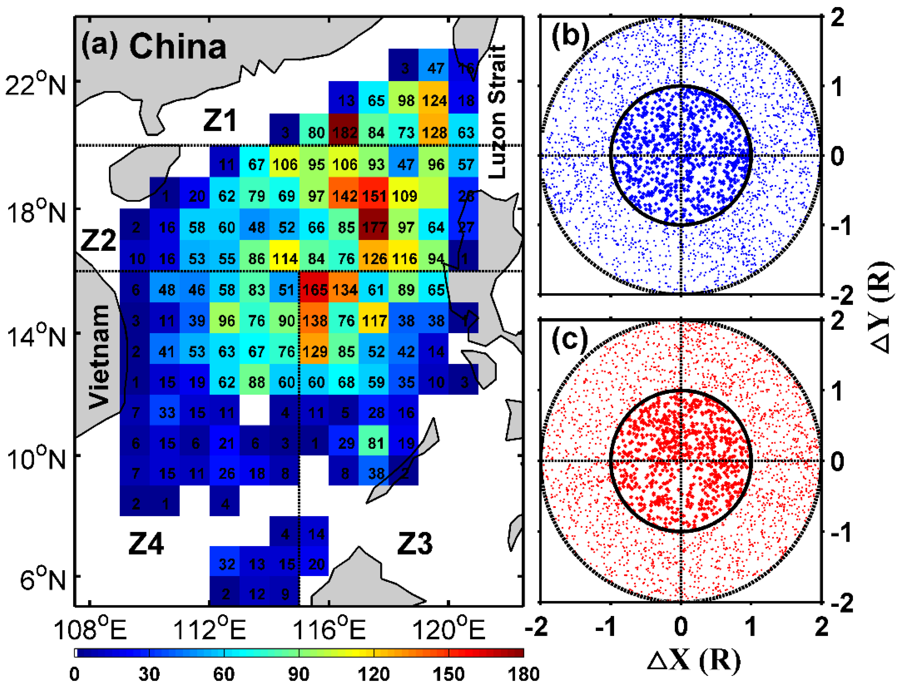
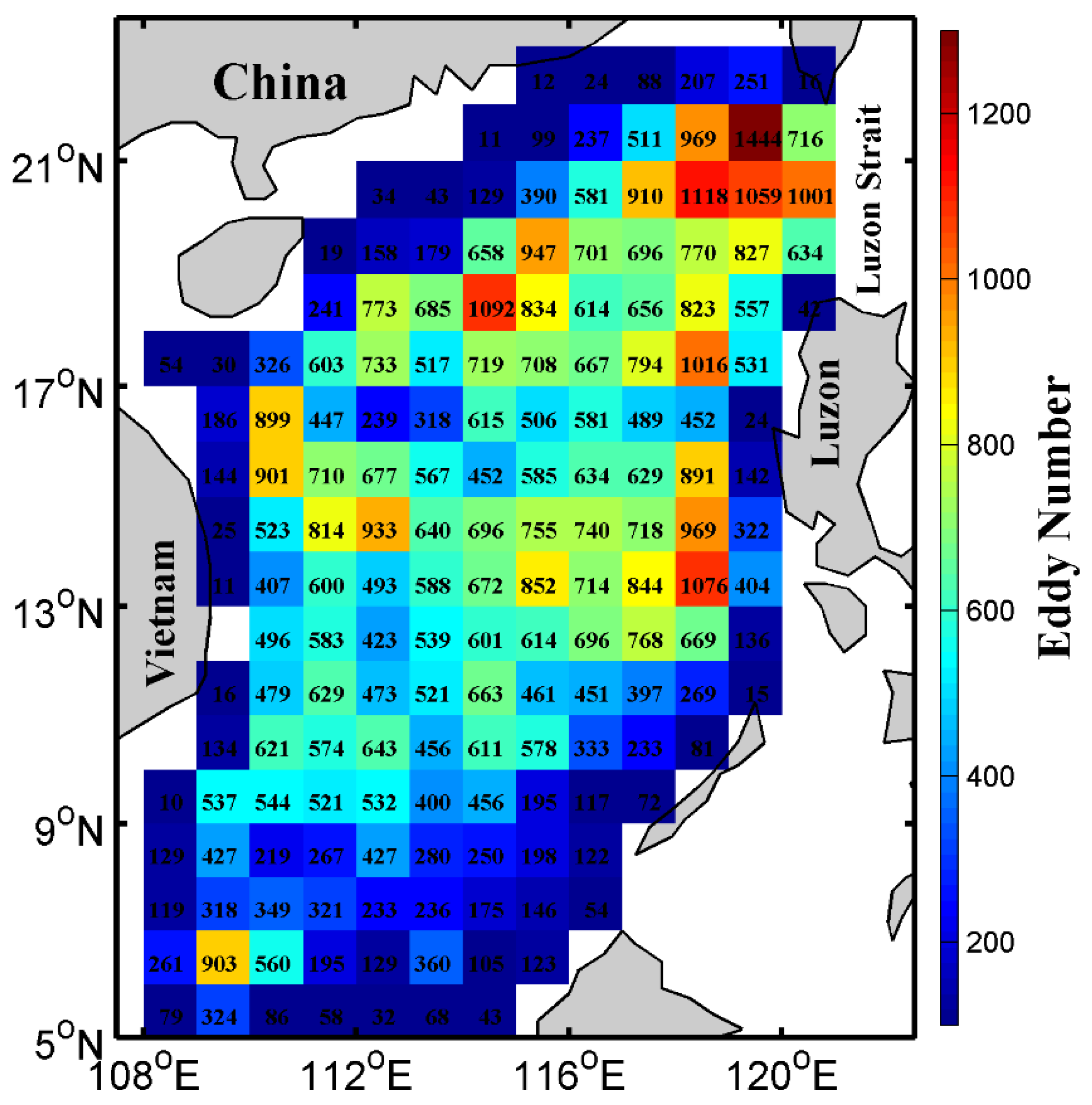
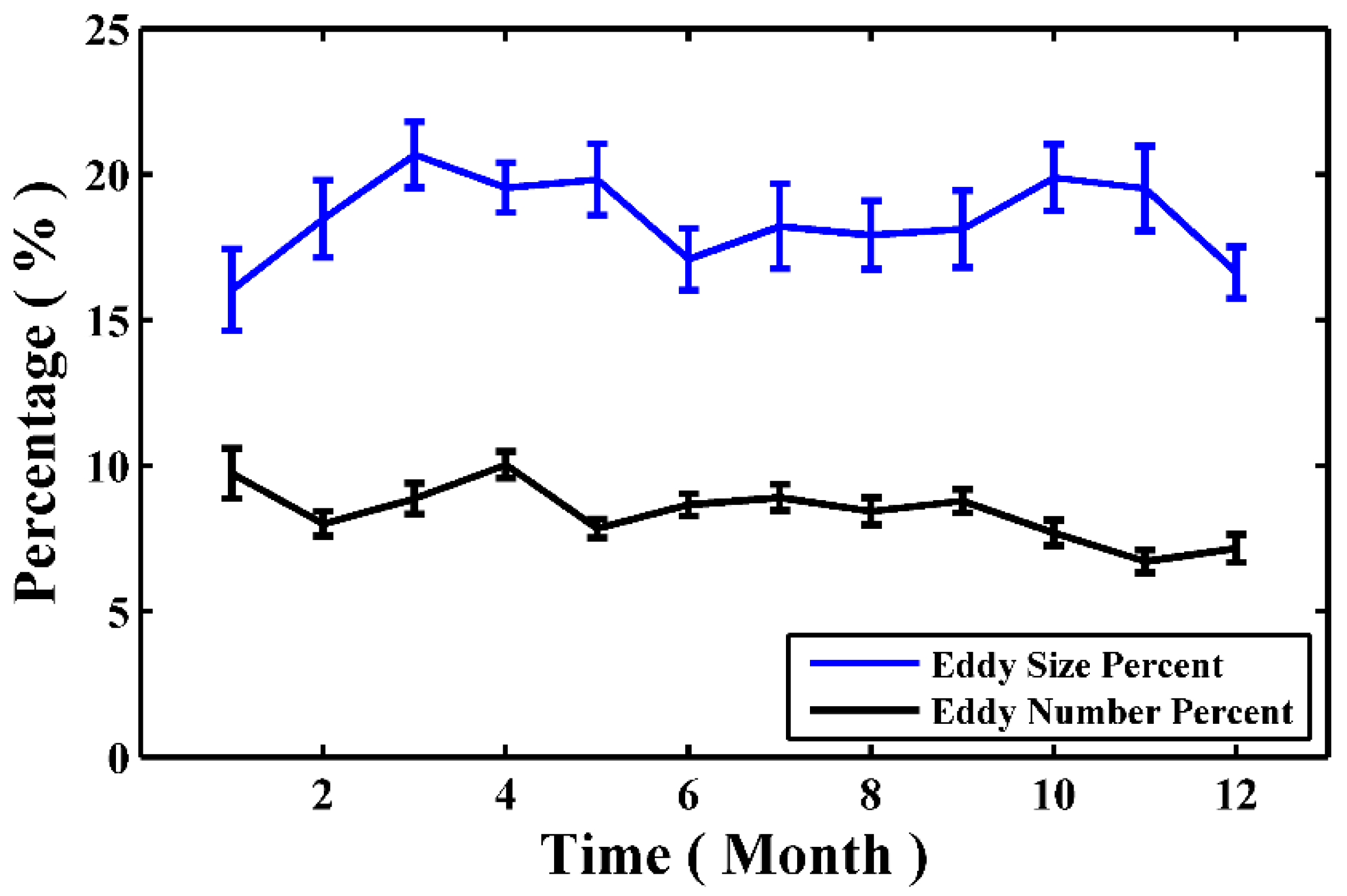
3.1. Eddy Distribution and Evolution

In total, 31,744 CEs (snapshot) and 29,324 AEs, corresponding to 603 (track) and 541 eddies with lifespans longer than or equal to 30 days, respectively, were detected in the SCS between 1 January 2005 and 31 December 2016. The number of CEs (snapshot) is larger than that of AEs which disagrees with results from Chen et al. [36] who suggested that there are more AEs. However, we find the number of CEs (2645.3±64.7, snapshot) larger than that of AEs (2443.7±63.2) in every year (not shown). The reason may be that the coarse temporal-spatial resolution (weekly, 1/3°×1/3°) of SSHA data they used likely missed more CEs which usually have shorter lifespans and smaller radius compared to AEs. Figure 2 presents eddy snapshots distribution in 1°×1° bin in the SCS. To make the figure clearer, bins with fewer than 10 eddies are omitted. Similar to Chen et al. [36], eddies mainly distribute in a northeast–southwest direction along the continental slope and southwest of Luzon Island. Furthermore, the largest distribution density may be located northwest of Luzon Strait, which is associated with the Kuroshio intrusion in this area [7,36]. It is worth noting that the eddies in subregion Z4 are sparse compared with Chen et al. [36], due to a different eddy detection method and temporal-spatial resolution (as mentioned above).

Some studies in other areas pointed out that oceanic mesoscale eddies occupied 25–30% of oceanic surface area [59]. Xiu et al. [35] suggested the mean area covered by eddies with depths greater than 1000 m was around 9.8% of the SCS area each year. Figure 3 illustrates the monthly variation of the percentage of eddy covered area occupying the whole size in the SCS. The mean area covered by eddies is 16.0–20.7% in the SCS, where the highest (lowest) percentage appears in March (January). The monthly average percentage (black line in the Figure 3) indicates that the number of eddies is almost the same during the whole year, suggesting a weak seasonal variation of eddy generation in the SCS.

In this study, the average radius is 72.5 ± 1.5 km for CEs and 73.4 ± 1.6 km for AEs, which is consistent with Chelton et al. [63]. Those results may be caused by eddies mainly concentrating between 13° N and 22° N in the SCS (Figure 2). Eddies with radius larger than 100 km account for 19.6% and 19.9% of CEs and AEs, respectively, and the radiuses of 4.3% CEs and 3.6% AEs are equal to or larger than 150 km. The largest CE is about 292.0 km and the largest AE is about 256.4 km. These eddies have an average lifespan of 52.6 ± 1.1 and 54.2 ± 1.4 days for CEs and AEs, respectively. It is worth mentioning that, although the majority of eddies survive for about 40 days, the longest lifespan of CE is 221 days and 267 days for AE. Those averaged radius and lifespan are smaller than reported by Chen et al. [36], (132 km and 8.8 weeks), which seems to indicate that the higher temporal-spatial resolution data correspond to the smaller and shorter lifespan eddies.

As mentioned by Liu et al. [50], Samelson et al. [64] and others, the eddy lifespan can be divided into three stages: youth stage (increasing rapidly), mature stage (stable) and aged stage (decreasing rapidly). The different stages of an eddy can be characterized by the evolution of its radius, kinetic energy (EKE), vorticity, eccentricity ratio and so on. In this study, the EKE is defined as the sum of kinetic energy within the eddy area, i.e., $\mathrm{EKE}={\displaystyle \sum _{i=1}^N\frac{u^2+v^2}{2}}$, where $N$ is the number of the points within the eddy area. The eddy vorticity (i.e., relative vorticity, $\zeta =\frac{\partial v}{\partial x}-\frac{\partial u}{\partial y}$) is selected as the maximum value of vorticity within an eddy boundary (the maximum positive value for CEs and the maximum absolute value for AEs). The eddy eccentricity ratio is defined by the inner ellipse of the eddy boundary, which is calculated as $\mathrm{Ecc}=\frac{a-b}{a}$, where $a$ and $b$ are the long and short axes of the ellipse, respectively. From the formula, the more circular the eddy shape, the smaller eddy eccentricity ratio is. To compare eddies with different lifespans, as in Liu et al. [50], each eddy age is normalized by its lifespan. Meanwhile, the four physical parameters introduced above also normalized by their respectively maximum value within each eddy lifespan. Figure 4 shows the normalized temporal evolution for these four physical parameters which is obtained by averaging all eddies with lifespan longer than or equal to 30 days.

It is obvious that the normalized eddy radius, EKE and vorticity increase rapidly in the youth stage (first 1/5 of an eddy’s lifespan), then stay relatively stable at mature stage (middle of the lifespan) and finally sharply decrease at the aged stage (last 1/5 of the lifespan) (Figure 4a–c). In contrast, the eccentricity ratio shows the opposite trend: at the youth stage, the rate decreases rapidly; then, it stays roughly constant at the mature stage; and, finally, it increases sharply before the eddy eventually dissipates (Figure 4d). The evolution of these physical parameters shows similar feature, regardless of the eddy type. We cannot simply compare the magnitudes between the CEs and AEs in Figure 4 because they are normalized by the maximum values within that eddy lifespan. The mean normalized eddy radius, EKE, vorticity, and eccentricity ratio are 0.6 ± 0.02, 0.3 ± 0.03, 0.7 ± 0.01, and 0.80 ± 0.05 for CEs and AEs, respectively, all these being the same for both CEs and AEs.

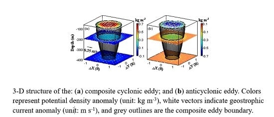
3.2. Composite 3-D Eddy Structure

Figure 5 shows the 3-D structures of the composite CE and AE in the SCS. The horizontal boundary of the composite eddy (the grey outlines) is defined as the outermost closed streamline around the eddy center with the velocity magnitude still increasing in the radial direction across its center [48]. The vertical depth of the composite eddy is considered as the depth of maximum geostrophic currents anomaly which is less than 0.02 m s⁻¹ inside the composite eddy horizontal boundary [40]. Figure 5 demonstrate that both composite CE and AE are bowl-shaped and have the thickness of about 400 m. Lin et al. [7] pointed out that the bowl-shaped eddies account for 65% of all eddies in this region by numerical simulation. The Argo data and composite method adopted in this study eliminate the possibility of other shapes (lens-shaped and cone-shaped).

The 3-D structure of the composite eddy has also been reported in other areas. With the aid of the numerical simulation, Dong et al. [51] also revealed three types of eddy shapes in the Southern California Bight, namely the bowl-shaped, lens-shaped and cone-shaped, with the largest eddy size on the surface, in the middle and at the bottom, respectively. All of these studies indicate that the composite eddies in the SCS may be thinner than those in other areas [65,66]. The findings of this 3-D structure of eddies promotes investigating the eddy-induced physical parameters anomalies as well as heat and freshwater transports (see Section 4 and Section 5).

4. Eddy-Induced Anomaly

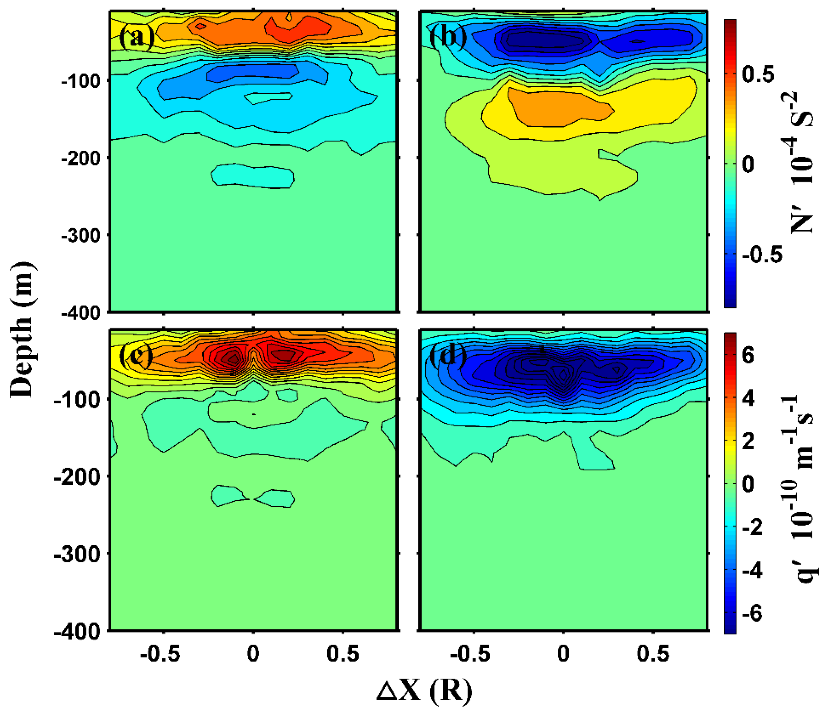
4.1. Eddy-Induced Geostrophic Current Anomaly

The geostrophic current of the composite eddy is calculated by the P-vector inverse method [67]. In this study, 1500 m is chosen as the reference depth. This method was used in many studies and reliable results were acquired [27,40,68,69]. The vertical sections of meridional geostrophic current anomaly component ($v$) across the composite eddy center along $\Delta \mathrm{Y}=0$ are shown in Figure 6a,b, and the horizontal sections of the composite eddies at depth 100 m are illustrated in Figure 6c,d. The geostrophic current anomaly presents a symmetric structure around the normalized eddy-coordinate center in each level (Figure 6a,b). In the vertical direction, $v$ is close to zero from the surface to the bottom through the normalized eddy-coordinate center in each layer. As is illustrated in the eddy detection method, along $\Delta \mathrm{Y}=0$ and passing through the composite eddy center, $v$ increases proportionally with increasing distance from the eddy center and decreases after reaching its maximum. As expected, the composite CE (Figure 6c) and AE (Figure 6d) are associated with a counterclockwise and clockwise rotational current field, respectively.

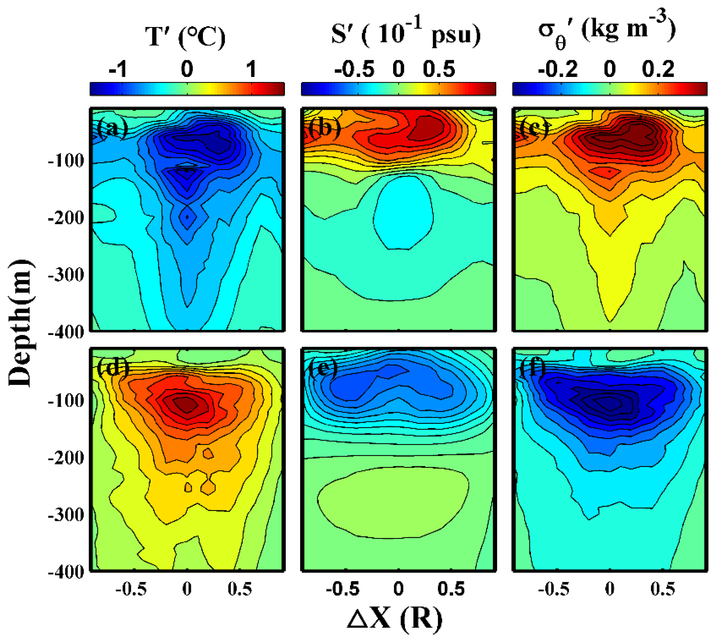
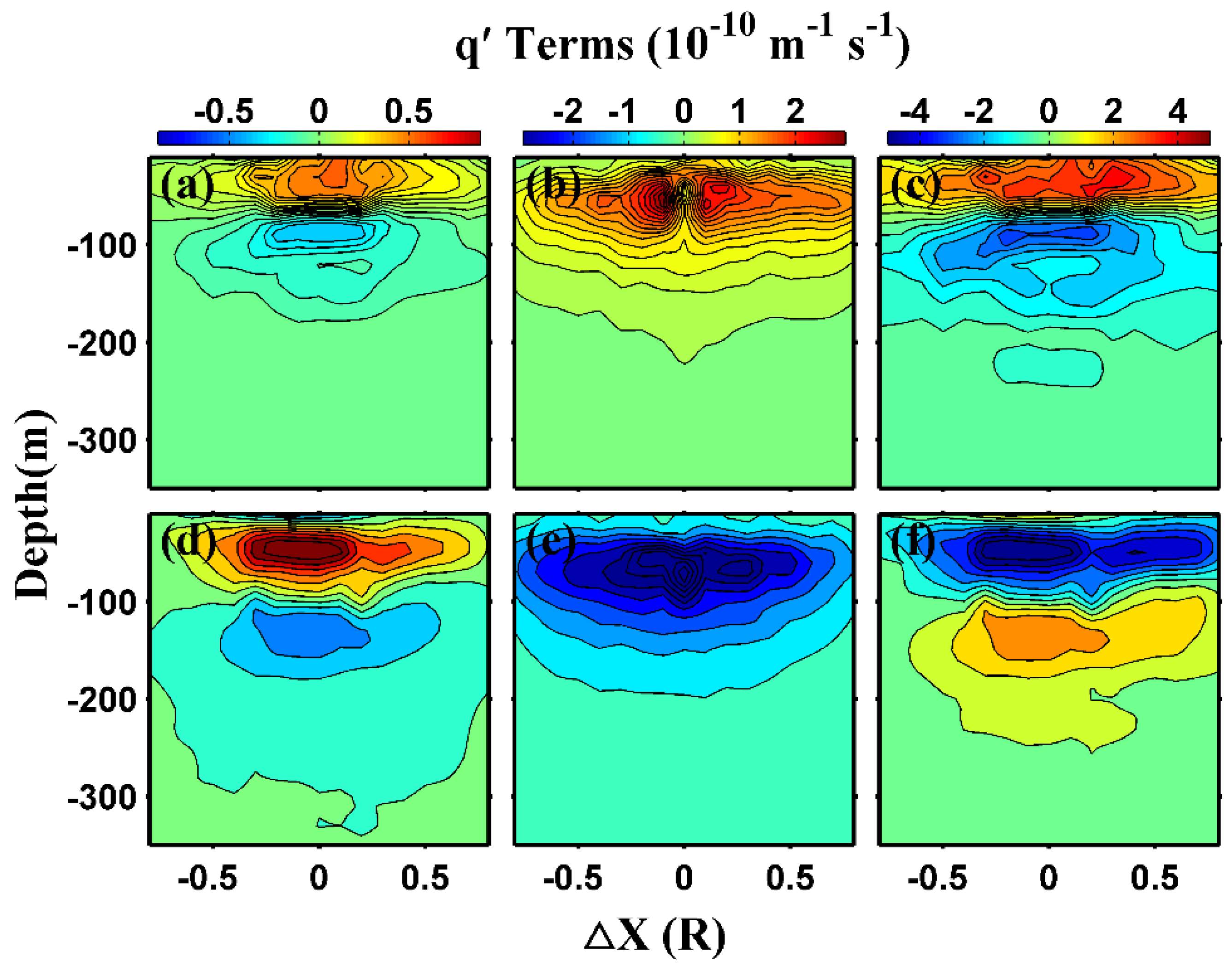
4.2. Eddy-Induced Temperature, Salinity and Potential Density Anomaly

Eddy-induced anomaly of the physical parameters can extend to the ocean interior [40]. Based on all the Argo profiles captured by eddies, Figure 7 gives the vertical profiles of average temperature anomaly ($\mathrm{T}\prime$), salinity anomaly ($\mathrm{S}\prime$), and potential density anomaly (${{\sigma }^{\prime }}_{\theta }$) within the eddy-coordinate system. As mentioned in Section 3.2, both composite eddies’ are about 400 m thick while an eddy’s influence can reach much deeper. From the sea surface to a depth of more than 1000 m, the composite CE corresponds to a negative $\mathrm{T}\prime$, while the composite AE is associated with a positive $\mathrm{T}\prime$ (not shown). The vertical distribution of $\mathrm{T}\prime$ is characterized by an increase with depth from the sea surface followed by a decrease after reaching its maximum. It should be noted from Figure 7a that the maximum $\mathrm{T}\prime$ is much shallower than that in the Kuroshio Extension region [40]. Maximum $\mathrm{T}\prime$ is about –0.7 °C (0.6 °C) centered at about 70 m (100 m) for the composite CE (AE). $\mathrm{T}\prime$ is obviously confined to the upper layer in the SCS.

The averaged vertical profiles of $\mathrm{S}\prime$ within the composite CE (blue solid curve) and AE (red solid curve) are presented in Figure 7b. Comparing Figure 7b with Figure 7a, there are three characteristics worth noting. First, $\mathrm{S}\prime$ has a two-layered structure changing sign at about 160 m. This two-layered structure is generated from the non-monotonic distribution of the oceanic salinity in the vertical direction. Second, the depth of maximum anomaly (in terms of magnitude) is located at about 50 and 60 m for the composite CE and AE, respectively, which is shallower for $\mathrm{S}\prime$ than that for $\mathrm{T}\prime$. Third, although the magnitude of $\mathrm{S}\prime$ for both composite CE and AE reaches almost 0.1 psu, it is small and negligible below 400 m, which demonstrates again that the eddy-induced changes are mainly confined to the upper layer.

Figure 7c presents the averaged vertical profiles of ${{\sigma }^{\prime }}_{\theta }$ obtained inside the composite eddies. The ${{\sigma }^{\prime }}_{\theta }$ modulated by the composite eddies has the same sign structure throughout the whole water column. The maximum ${{\sigma }^{\prime }}_{\theta }$ inside the composite CE is about 0.2 kg m⁻³ at 60 m, while that inside the composite AE is −0.2 kg m⁻³ at about 80 m. The composite CE (AE) creates a lower (higher) temperature and higher (lower) salinity in the upper 160 m, which cause the corresponding increase (decrease) in potential density. Sun et al. [40] pointed out that the composite CE (AE) modulated the lower (higher) temperature and lower (higher) salinity in the upper layer, which has the opposite impact on potential density. Therefore, the impact of temperature and salinity results in little change of potential density in the Kuroshio Extension region. In the SCS, consistent change of temperature and salinity induced by mesoscale eddies co-determines the larger change of potential density in the upper layer of the SCS. In the depth between 160 m and 430 m, the impact of $\mathrm{T}\prime$ and $\mathrm{S}\prime$ on ${{\sigma }^{\prime }}_{\theta }$ is opposite. The variation trend of ${{\sigma }^{\prime }}_{\theta }$ is the same as $\mathrm{T}\prime$ in those depth, which implies the impact of $\mathrm{T}\prime$ on ${{\sigma }^{\prime }}_{\theta }$ is larger than that of $\mathrm{S}\prime$.

Figure 7 also gives the $\mathrm{T}\prime$ and $\mathrm{S}\prime$ in the four subregions. The variation trend of $\mathrm{T}\prime$ and $\mathrm{S}\prime$ are almost the same in each subregion. However, an interesting characteristic about $\mathrm{S}\prime$ in subregion Z1 should be noted. The $\mathrm{S}\prime$ induced by the cyclonic (anticyclonic) eddy is associated with negative (positive) salinity anomaly in the upper layer. This variation of $\mathrm{S}\prime$ is opposite to other subregions (Z2, Z3, and Z4). It implies that the eddy-induced freshwater transport is opposite in other subregions (see Section 5). These salinity anomaly profiles (in subregion Z1) correspond to those observed in the Kuroshio Extension region [40], and are thus indicative of the fact that waters with high temperature and high salinity from the Kuroshio might be intruding in this area [7,36]. This is an important finding and needs more attention in future study.

Figure 8 shows vertical sections of the composite eddies along $\Delta \mathrm{Y}=0$ and across the composite eddy center. The changes of oceanic physical parameters are mainly confined to one times the normalized radius around the composite eddy center in the meridional direction and within the upper 400 m in the vertical direction. We approximate the bottom of the composite eddy as 400 m, since the physical parameters within an oceanic eddy are strikingly different from its ambient environment until this depth. Contrasting Figure 8a (Figure 8d) with Figure 8b (Figure 8e), the composite eddy-modulated $\mathrm{T}\prime$ has a consistent change at all depth, while $\mathrm{S}\prime$ has an opposite change at below and above about 160 m, as we mention above. The maximum change of $\mathrm{T}$, $\mathrm{S}$ and ${\sigma }_{\theta }$ within the composite CE reaches −1.5 °C at about 70 m, 0.1 psu at about 50 m, and 0.5 kg m⁻³ at about 60 m, respectively. In contrast, the maximum change of T, S and ${\sigma }_{\theta }$ in the composite AE reaches 1.6 °C at about 110 m, −0.1 psu at about 70 m, and −0.5 kg m⁻³ at about 90 m, respectively.

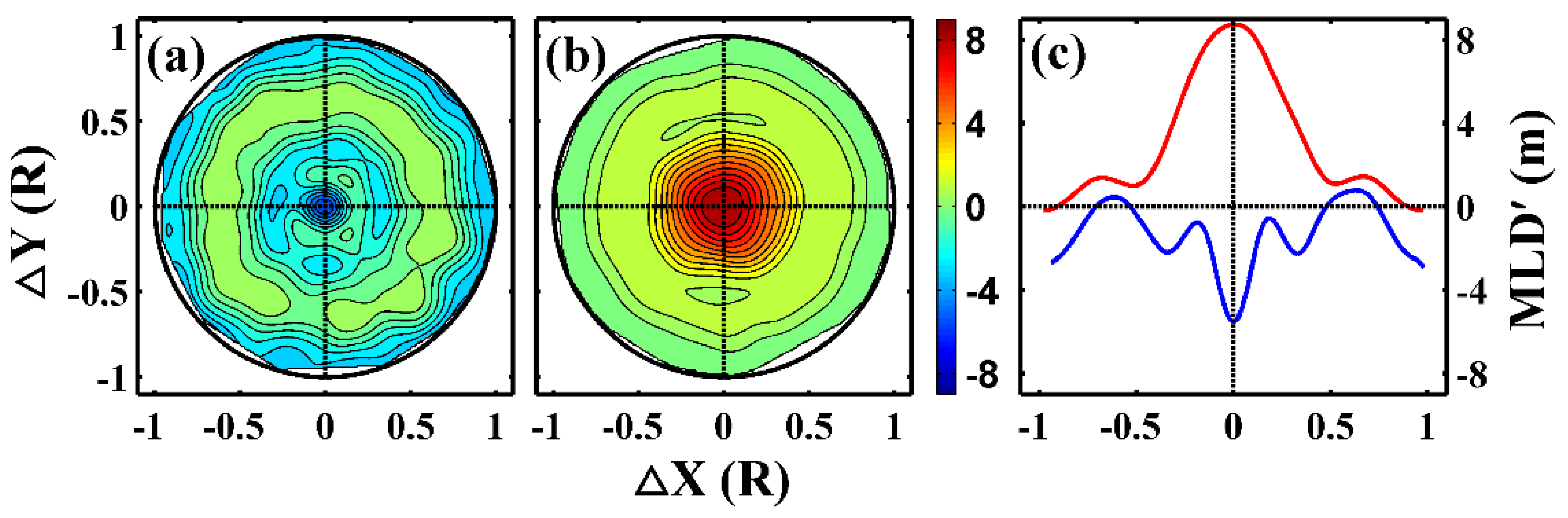
4.3. Composite Eddy-Modulated Mixed Layer Depth Anomaly

As mentioned in Section 4.2, the composite eddy modulates obvious anomaly T, S and ${\sigma }_{\theta }$ within eddies. The composite eddy also modulates changes in other physical parameters within the eddy, such as mixed layer depth (MLD), buoyancy frequency (N), and potential vorticity (PV). Furthermore, we can presume that the composite eddy-modulated changes about other physical parameters also mainly focus on the upper layer. In this subsection, we discuss in detail the anomaly associated with the composite eddies in terms of MLD. The composite eddy modulated N and PV anomaly will be illustrated in details in Section 6.

Figure 9a,b reveals the averaged MLD anomaly modulated by the composite CE and AE, respectively, and Figure 9c gives MLD anomaly across the composite eddy center along $\Delta \mathrm{Y}=0$. The composite CE- and AE-modulated maximum anomaly of MLD are 5.5 and 8.7 m, respectively, both appearing in the center of the composite eddies. As the climatological MLD in the SCS is about 27.2 m (calculated from all available Argo profiles in the SCS), it means the composite CE- and AE-modulated maximum MLD anomaly are about 20.2% and 32.0%, respectively. The eddy-induced MLD variation in the South China Sea (5.5 m for composite CE and 8.7 m for composite AE) is shallower than that in the Kuroshio Extension region (11.6 m for composite CE and 18.5 m for composite AE, Sun et al. [40]) However, in terms of percentage change modulated by the composite eddy, there are no obvious differences between them (23.6% for composite CE and 38.4% for composite AE in Kuroshio Extension region). It is visible in Figure 9c that MLD anomaly modulated by the composite eddy is just like a parabola whose vertex is located at the composite eddy center.

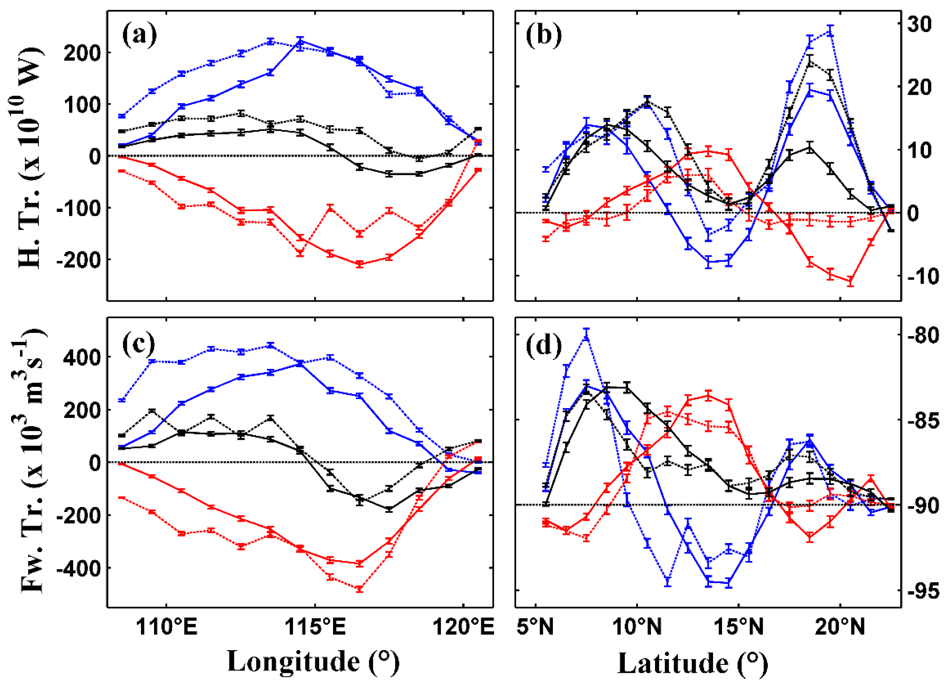
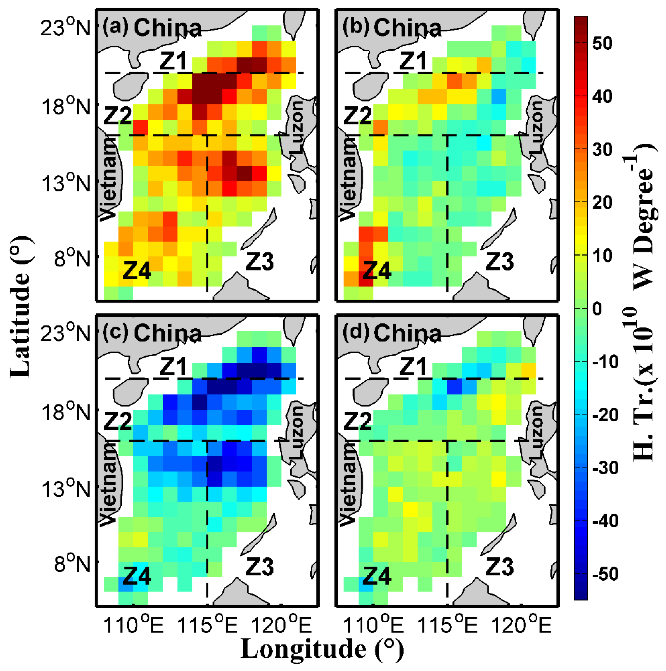
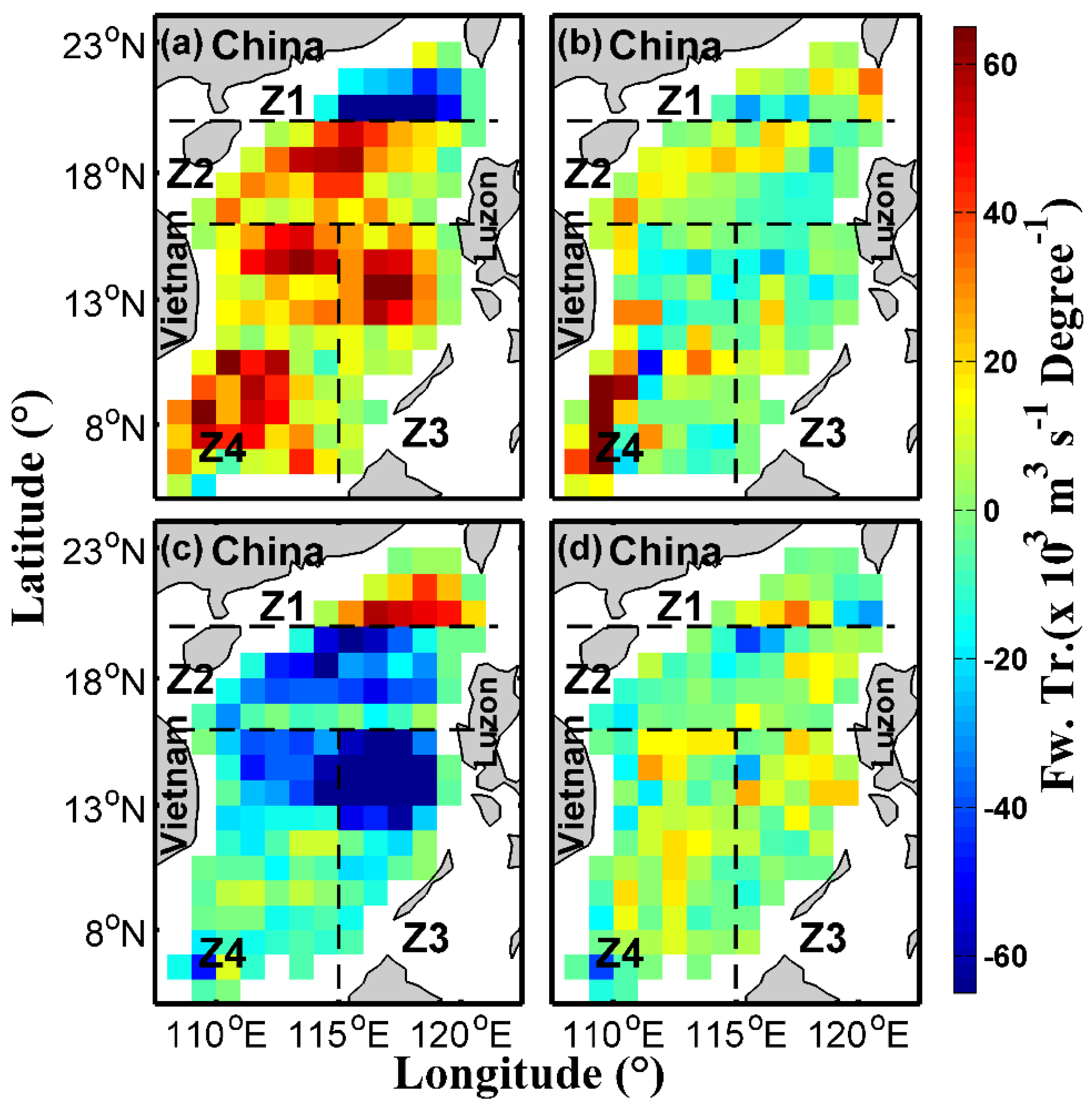
5. Eddy-Induced Heat and Freshwater Transports

Figure 10 presents the eddy-induced heat and freshwater transports in the SCS area. The largest time-averaged heat transport, induced by CE in zonal direction, is about (222.8 ± 6.2) × 10¹⁰ W which is integrated in the meridional direction with 1° width (Figure 10a, blue solid curve). Correspondingly, that AE-induced is about (209.9 ± 5.92) × 10¹⁰ W (Figure 10a, red solid curve). Overall, the CE-induced eastward heat transport and AE-induced westward heat transport almost offset each other. In detail, west of about 117° E the eddy-induced heat transport is eastward, while east of that longitude the heat transport is westward. At the whole SCS scale, the heat transport induced by the eddy is generally eastward (Figure 10a, black solid curve).

Figure 10c,d shows similar patterns to Figure 10a,b, respectively, because, as mentioned above, the eddy-induced $\mathrm{T}\prime$ and $\mathrm{S}\prime$ have very similar patterns in the vertical direction. The maximum freshwater transport by CEs reaches (373.6 ± 9.7) × 10³ m³ s⁻¹ and (384.2 ± 10.8) × 10³ m³ s⁻¹ by AEs, corresponding to $(8.5\pm 0.2)$% and $(8.7\pm 0.2)$% of the annual mean Luzon Strait transport, respectively (about 4.4 Sv, 1 Sv = 10⁶ m³ s⁻¹ according to Fang et al. [70] and Nan et al. [71]). Even though this brings a certain degree of uncertainty, the results shown in this study do not affect the conclusion that the eddy-modulated heat and freshwater transports plays a crucial role in the SCS. To validate our results, Figure 10 (dashed curves) also gives the results derived from the method proposed by Dong et al. [22]. As shown in Figure 10, the magnitudes of eddy-induced heat and freshwater transports are consistent in both methods.

The distribution of the meridional heat transport induced by the eddy is much complex than that in the zonal direction. The heat transport in meridional direction can be divided into three sections: south of 11° N, the cyclonic eddy-induced northward heat transport (Figure 10b, black solid curve); from 11° N to 17° N, the total heat transport is very small, resulting from the positive transport by the AE (Figure 10b, red solid curve) and the negative transport by the CE (Figure 10b, blue solid curve) offsetting each other; and north of 17°N, the northward heat transport mainly rests in the CE.

Figure 11 gives the eddy-induced heat transport in each 1°×1° bin, from which we know the CE- and AE-induced zonal heat transport is positive (Figure 11a) and negative (Figure 11c) in general, respectively. The positive value means that the zonal heat transport is eastward which stems from the westward eddy movement and its negative temperature anomaly (Figure 7a, blue solid curve). Conversely, the negative heat transport modulated by AE, meaning the AE transport heat westward which is caused by the AE’s west movement velocity and its positive temperature anomaly (Figure 7a, red solid curve). Comparing Figure 11a or Figure 11c with Figure 2, we found that they have the similar patterns: the maximum value both appearing at the northwest continental shelf area and the southwest area of Luzon Island. The distribution of zonal heat transport related to eddy is dependent on the intensity of the eddy activity. In Figure 11b (Figure 11d), along the northwest boundary, the meridional heat transport is positive (negative), while it is negative (positive) in other areas.

Figure 12 gives the distribution of eddy-induced freshwater transport in each 1°×1° bin. Comparing Equations (1) and (2), it is clear that the difference between eddy-induced heat and freshwater transports mainly depends on the vertical profile of $\mathrm{T}\prime$ and $\mathrm{S}\prime$, both following a similar pattern (Figure 7a,b). Comparing Figure 12a,c with Figure 11a,c, there are two significant characteristics worth noting. (1) The eddy-induced freshwater transport in subregion Z1 is opposite to other subregions (as mentioned in Section 4.2). The opposite variation of $\mathrm{S}\prime$ in subregion Z1 and other subregions can account for this distribution. This finding is very interesting and could be used to study the Kuroshio intrusion in future study. (2) The eddy induced freshwater transport is significantly strengthened in the Z3 area (near the Luzon Island). Considering the eddy-induced salinity anomaly in Z3 area is larger than that in other subregions (Figure 7b), this distribution of the freshwater transport is easy to understand. The eddy-induced meridional freshwater transport (Figure 12b,d) also has those two characteristics, although not very significant.

6. Discussion

Buoyancy frequency ($\mathrm{N}=\sqrt{-\frac{g}{\rho }\frac{\partial \rho }{\partial z}}$) reflects the oceanic stratification in the vertical direction, and limits the maximum frequency of oceanic internal wave. Nurser and Zhang [72] found that eddy could change the pre-existing oceanic stratification by eddy-induced upwelling or downwelling within the eddy. Figure 13a,b describes the vertical section of buoyancy frequency squared anomaly (${\mathrm{N}}^2{}^{\prime }$) along the zonal direction ($\Delta \mathrm{Y}=0$) across the composite eddy center. The most outstanding characteristic from Figure 13a,b is that ${\mathrm{N}}^2{}^{\prime }$ has a two-layer structure for both composite CE and AE (the upper layer is obviously stronger than the lower one). The composite CE-modulated maximum increase of ${\mathrm{N}}^2{}^{\prime }$ is $6.3\times {10}^{-5}$ s⁻² at about 30 m and the maximum decrease is $-4.7\times {10}^{-5}$ s⁻² at about 100 m (Figure 13a), while the composite AE-modulated maximum increase of ${\mathrm{N}}^2{}^{\prime }$ is $4.6\times {10}^{-5}$ s⁻² at about 130 m and the maximum decrease is $-8.7\times {10}^{-5}$ s⁻² at about 40 m (Figure 13b).

Those two-layer structures suggest that the composite CE (AE) compresses (stretches) the pre-existing stratification above 70 (80) m, while it stretches (compresses) the pre-existing stratification below that depth. The upwelling modulated by the composite CE brings sea water from the thermocline into the mixed layer and then strengthens the vertical stratification in the upper 70 m while it weakens the vertical stratification below 70 m because of the loss of high-density water mass. On the other hand, the composite AE causes a similar but opposite progress, i.e., the downwelling modulated by the composite AE press-in sea water from the mixed layer into the thermocline and then weakens the vertical stratification in the upper 80 m, while it strengthens the vertical stratification below 80 m because of the obtained low-density water mass.

Potential vorticity (PV) is calculated by the formula: $q=-\frac{f+\zeta }{{\rho }_0}\frac{\partial \rho }{\partial z}$, where $f$ is the vertical component of planetary vorticity, $\zeta$ is the vertical component of relative vorticity calculated by $\zeta =\frac{\partial v}{\partial x}-\frac{\partial u}{\partial y}$, and ${\rho }_0$ is the reference density valued at 1,025 kg m⁻³. $u$ and $,v$ are the geostrophic velocity anomaly component in zonal and meridional direction, respectively. Figure 13c,d presents the vertical section of potential vorticity anomaly ($q^{\prime }$) across the composite eddy center and along $\Delta \mathrm{Y}=0$. $q^{\prime }$ is defined as the D-value between the potential vorticity within eddy ($q_{eddy}$) and the background potential vorticity ($q_{bg}$). It is demonstrated that the composite CE-modulated $q^{\prime }$ has a clear two-layer structure and the upper layer is stronger than the lower one (Figure 13c). However, the composite AE-modulated $q^{\prime }$ is small and negligible below about 100 m and presents almost a one-layer structure (Figure 13d). The composite CE-modulated maximum positive $q^{\prime }$ is $7.6\times {10}^{-10}$ m⁻¹ s⁻¹ at about 40 m and the maximum negative $q^{\prime }$ is $-0.7\times {10}^{-10}$ m⁻¹ s⁻¹ at about 100 m, while the composite AE-modulated maximum positive $q^{\prime }$ is $9.3\times {10}^{-11}$ m⁻¹ s⁻¹ at about 150 m and maximum negative $q^{\prime }$ is $-9.8\times {10}^{-10}$ m⁻¹ s⁻¹ at about 50 m. From the PV definition, both relative vorticity ($\zeta$) and gradient of potential density ($\frac{\partial \rho }{\partial z}$) could induce PV change. Sun et al. [40] suggested that the two-layer structure of $q^{\prime }$ depends on the vertical potential density gradient anomaly. The vertical potential density gradient can reflect stratification of the ocean, which is seen as an intimate bond between $q^{\prime }$ and stratification.

As PV plays a vital role in explaining eddy’s movement direction, stability and other features, we will give a detailed discussion on the composite eddy-modulated $q^{\prime }$ in this section. On the one hand, PV gradient generally induces a westward displacement for eddies (both CE and AE), with an additional northward or southward component for CE or AE, respectively [73]. On the other hand, PV (more precisely Ertel PV) is the key quantity for diagnosing eddy instability. An eddy is unstable to symmetric instability when its PV is negative [74,75,76]. The composite eddy-modulated $q^{\prime }$ can be calculated by:

$$\begin{array}{l}{q}^{\prime }=q_{eddy}-q_{bg}\\ =(-\frac{{\zeta }_{eddy}+f}{{\rho }_0}\frac{\partial {\rho }_{eddy}}{\partial z})-(-\frac{{\zeta }_{bg}+f}{{\rho }_0}\frac{\partial {\rho }_{bg}}{\partial z})\\ =\frac{\rho {\zeta }_{eddy}}{g{\rho }_0}(-\frac{g}{\rho }\frac{\partial {\rho }_{eddy}}{\partial z}+\frac{g}{\rho }\frac{\partial {\rho }_{bg}}{\partial z})+\frac{\rho f}{g{\rho }_0}(-\frac{g}{\rho }\frac{\partial {\zeta }_{eddy}}{\partial z}+\frac{g}{\rho }\frac{\partial {\rho }_{bg}}{\partial z})-\frac{\rho {\zeta }_{eddy}}{g{\rho }_0}\frac{g}{\rho }\frac{\partial {\rho }_{eddy}}{\partial z}+\frac{\rho {\zeta }_{bg}}{g{\rho }_0}\frac{g}{\rho }\frac{\partial {\rho }_{bg}}{\partial z}\\ =\frac{\rho }{g{\rho }_0}{\zeta }_{eddy}{N}^2{}^{\prime }+\frac{\rho }{g{\rho }_0}f{N}^2{}^{\prime }+\frac{\rho }{g{\rho }_0}({\zeta }_{eddy}-{\zeta }_{bg})N_{bg}^2\\ =\frac{\rho }{g{\rho }_0}{\zeta }_{eddy}{N}^2{}^{\prime }+\frac{\rho }{g{\rho }_0}{\zeta }_{eddy}{N}_{bg}^2+\frac{\rho }{g{\rho }_0}f{N}^2{}^{\prime },\end{array}$$

(5)

where $q_{eddy}$ is the potential vorticity within the eddy and $q_{bg}$ is the background potential vorticity. We assume the background relative vorticity is equal to zero (${\zeta }_{bg}=0$) in this study. Following the above equation, $q^{\prime }$ can be divided into three terms.

To illustrate the effect of each term on $q^{\prime }$, Figure 14 gives the vertical sections of those terms across the composite eddy center along $\Delta \mathrm{Y}=0$. For the composite CE, both the first (Figure 14a) and the third (Figure 14c) terms are characterized by a two-layer structure with their upper layers (shallower than about 50 m) displaying positive values and the lower layers (deeper than about 50 m) negative values, while the second term only has a single layer with the positive values. Because it is obvious from Formula (5) that ${\zeta }_{eddy}$ associated with CE and $f$ are positive at all depth (northern hemisphere), we can deduce that the two-layer structure in Figure 14a,c must be induced by ${\mathrm{N}}^2{}^{\prime }$ (Figure 13a). In a depth shallower than 50 m, given that each of the three terms induces a positive potential vorticity change, then the composite CE makes an intense $q^{\prime }$ in the upper layer (Figure 13c). However, in the lower layer (deeper than 60 m), the opposite change (the first and third term exhibit negative change, but the second term shows positive change) leads to an obviously weaker $q^{\prime }$ than that in the upper layer (Figure 13c).

The composite AE-modulated $q^{\prime }$ also have a two-layer structure for the first (Figure 14d) and the third (Figure 14f) term, but their phase is opposite to each other. Therefore, the first and the third term will weaken each other at all depths. The second term is characterized by negative anomaly at all depths, which is consistent with the composite AE having a clockwise current field (Figure 6d). The composite AE-modulated negative changes in the second and the third term eliminate the positive change in the first term in the upper layer (shallower than about 70 m) resulting in $q^{\prime }$ presenting negative change, while the positive change in the third term eliminates the negative changes in the first and the second term to induce a weak positive change in the lower layer (Figure 13d).

Although PV is a 3-D vector, we only discuss its vertical component, because of the limited resolution of the data. In fact, seeing that the horizontal component of PV plays an important role in the stability of the oceanic mesoscale eddy [74,75,76], high-resolution numerical simulation will be utilized in the future to study the eddy-induced 3-D PV change.

In addition, the MLD anomaly are also strongly influenced by the submesoscale process [46,77,78,79]. Zhang et al. [34] proposed that the mesoscale eddy would release most energy to submesoscale process, and the latter would induce intense mixing and then change the MLD. However, the resolution of our data is obviously not enough to study the MLD anomaly induced by submesoscale processes, which is a very interesting future study requiring high-resolution data from observation and/or numerical modeling.

7. Conclusions

In this study, we focused on the eddy’s surface features, 3-D structures, impacts on oceanic physical parameters and heat/freshwater transports in the SCS. Studying 12 years of satellite altimetry data, we find that mesoscale eddies occupy 16.0%–20.7% of the sea surface area and mainly concentrate in the northwestern area in the SCS and southwest of Luzon Island. The average radial size and lifespan for CEs are 72.5 ± 1.5 km and 52.6 ± 1.1 days and those for AEs are 73.4 ± 1.6 km and 54.2 ± 1.4 days, respectively. Those radius and lifespans are smaller than the ones reported by Chen et al. [36] (132 km and 8.8 weeks). This difference might come from the different temporal-spatial resolution data and the different eddy detection methods used in those two studies.

As suggested by Liu et al. [50], the eddy lifespan can be divided into three stages: radial size, EKE and relative vorticity increase rapidly in the youth stage, remain relative stable in the mature stage and decrease quickly in the aged stage. The eddy eccentricity ratio presents the opposite variation trend to the eddy radial size, EKE and vorticity, which indicates that, in the mature stage, the eddy shape is closer to a circle than that in the youth and aged stage.

By satellite altimetry and Argo profiles data, the 3-D structure of the composite eddies are revealed. Using the composite analysis method, we found that both composite CE and AE are bowl-shaped and extend to about 400 m in the vertical direction. The composite CE and AE correspond to the counterclockwise and clockwise current field, respectively, and the magnitude of their swirl speed is on the order of 0.1 m s⁻¹ on the eddy surface. At the composite eddy center, the composite CE-modulated maximum change of T, S and ${\sigma }_{\theta }$ are −1.5 °C (at about 70 m), 0.1 psu (at about 50 m), and 0.5 kg m⁻³ (at about 60 m), respectively, while the composite AE-modulated maximum T, S and ${\sigma }_{\theta }$ are 1.6 °C (at about 90 m), −0.1 psu (at about 70 m), and −0.5 kg m⁻³ (at about 90 m), respectively. Although the composite CE- (AE-) modulated $\mathrm{T}\prime$, $\mathrm{S}\prime$ and ${{\sigma }^{\prime }}_{\theta }$ can extend to more than 1000 m, those changes all focus on the upper 400 m. In contrast to the temperature situation, the distribution of oceanic salinity is not monotonous in the vertical direction, which makes $\mathrm{S}\prime$ exhibit a two-layer structure, i.e., positive (negative) above 160 m, but negative (positive) below that depth.

At the composite eddy center, the composite CE-modulated (AE-modulated) MLD shallows by 5.5 m (deepens by 8.7 m), corresponding to 20.2% (32.0%) of the climatological MLD in the SCS. The composite eddy not only modulates the MLD changes but also lead to changes in ${\mathrm{N}}^2$ and PV within the composite eddies. The ${\mathrm{N}}^2{}^{\prime }$ associated with the composite eddy is characterized by a two-layer structure where the phases of the composite CE and AE are opposite to each other. In other words, the composite CE is positive in the upper layer and negative in the lower layer, while the composite AE is negative in the upper layer and positive in the lower layer. The order of ${\mathrm{N}}^2{}^{\prime }$ is O (10⁻⁴ s⁻²), similar to ${\mathrm{N}}_{bg}^2$ in the SCS. The positive PV change modulated by the composite CE can extend to about 70 m, while that modulated by the composite AE reaches about 120 m. We divide the composite eddy-modulated $q^{\prime }$ into three terms: (1) the interaction between ${\zeta }_{eddy}$ and ${\mathrm{N}}^2{}^{\prime }$; (2) the interaction between ${\zeta }_{eddy}$ and ${\mathrm{N}}_{bg}^2$; and (3) the interaction between $f$ and ${\mathrm{N}}^2{}^{\prime }$.

The heat and freshwater transports induced by oceanic mesoscale eddy is also discussed in the study. In the SCS, the CE-induced eastward heat transport and the AE-induced westward heat transport almost offset each other. Moreover, the zonal heat transport induced by the eddy is not significant. The zonal freshwater transport induced by CE and AE is (373.6 ± 9.7) × 10³ m³ s⁻¹ and (384.2 ± 10.8) × 10³ m³ s⁻¹, respectively, which is equivalent to (8.5±0.2)% and (8.7±0.2)% of the annual mean transport through the Luzon Island. This result indicates that the eddy plays a critical role in mass transport in the SCS, findings which must be considered in other relevant researches.

These results provide a full-scale understanding of mesoscale eddies in the SCS. Revealed characteristics of eddy spatial distribution can provide guides to deploy the reference for placing buoys for relevant researches. By illustrating the 3-D structure of the composite eddy, the information is available for studying the effect of mesoscale eddy on oceanic physical parameters (e.g., eddy induced heat/salt/freshwater transports) in this region. The discussion of PV changes modulated by the composite eddy promotes our understanding of eddy dynamic processes in the upper ocean. Due to the limited resolution of data, the submesoscale process, which plays a vital role in oceanic eddy stability, is not addressed in this study but will be the emphasis of future work.

References

1. Su, J.; Xu, J.; Cai, S.; Wang, O. Gyres and eddies in the South China Sea. In Onset and Evolution of the South China Sea Monsoon and Its Interaction with the Ocean; Ding, Y., Li, C., Eds.; Meteorol. Press: Beijing, China, 1999; pp. 272–279. [Google Scholar]
2. Shaw, P.T.; Chao, S.Y.; Fu, L. Sea surface height variations in the South China Sea from satellite altimetery. Oceanol. Acta 1999, 22, 1–17. [Google Scholar] [CrossRef]
3. Hwang, C.; Chen, S. Circulations and eddies over the South China Sea derived from TOPEX/Poseidon altimetry. J. Geophys. Res. 2000, 105, 23943–23965. [Google Scholar] [CrossRef]
4. Wang, G.; Su, J.; Chu, P.C. Mesoscale eddies in the South China Sea detected from altimeter data. Geophys. Res. Lett. 2003, 30, 2121. [Google Scholar] [CrossRef]
5. Faghmous, J.H.; Frenger, I.; Yao, Y.; Warmka, R.; Lindell, A.; Kumar, V. A daily global mesoscale ocean eddy dataset from satellite altimetry. Sci. Data 2015, 2. [Google Scholar] [CrossRef] [PubMed]
6. Sun, M.; Tian, F.; Liu, Y.; Chen, G. An improved automatic algorithm for global eddy tracking using satellite altimeter data. Remote Sens. 2017, 9, 206. [Google Scholar] [CrossRef]
7. Lin, X.; Dong, C.; Chen, D.; Liu, Y.; Yang, J.; Zou, B.; Guan, Y. Three-dimensional properties of mesoscale eddies in the South China Sea based on eddy-resolving model output. Deep Sea Res. 2015, 99, 46–64. [Google Scholar] [CrossRef]
8. Dale, W. Wind and drift current in the South China Sea. Malaysian J. Trop. Geogr. 1956, 8, 1–31. [Google Scholar]
9. Chelton, D.B.; Schlax, M.G.; Samelson, R.M.; De Szoeke, R.A. Global observations of large oceanic eddies. Geophys. Res. Lett. 2007, 34, 87–101. [Google Scholar] [CrossRef]
10. Chelton, D.B.; Gaube, P.; Schlax, M.G.; Early, J.J.; Samelson, R.M. The influence of nonlinear mesoscale eddies on near-surface oceanic chlorophyll. Science 2011, 334, 328–332. [Google Scholar] [CrossRef] [PubMed]
11. Chen, G.; Gan, J.; Xie, Q.; Chu, X.; Wang, D.; Hou, Y. Eddy heat and salt transports in the South China Sea and their seasonal modulations. J. Geophys. Res. 2012, 117. [Google Scholar] [CrossRef]
12. Gaube, P.; McGillicuddy, D.J.; Chelton, D.B.; Behrenfeld, M.J.; Strutton, P.G. Regional variations in the influence of mesoscale eddies on near-surface chlorophyll. J. Geophys. Res. 2014, 119. [Google Scholar] [CrossRef]
13. Dong, C.; McWilliams, J.C.; Liu, Y.; Chen, D. Global heat and salt transports by eddy movement. Nat. Commun. 2014, 5. [Google Scholar] [CrossRef] [PubMed]
14. Zhang, Y.; Liu, Z.; Zhao, Y.; Wang, W.; Li, J.; Xu, J. Mesoscale eddies transport deep-sea sediments. Sci. Rep. 2014, 4, 5937. [Google Scholar] [CrossRef] [PubMed]
15. Zhang, Z.; Wang, W.; Qiu, B. Oceanic mass transport by mesoscale eddies. Science 2014, 345, 322–324. [Google Scholar] [CrossRef] [PubMed]
16. Zhang, Z.; Zhong, Y.; Tian, J.; Yang, Q.; Zhao, W. Estimation of eddy heat transport in the global ocean from Argo data. Acta Oceanol. Sin. 2014, 33, 42–47. [Google Scholar] [CrossRef]
17. He, Q.; Zhan, H.; Cai, S.; Li, Z. Eddy effects on surface chlorophyll in the northern South China Sea: Mechanism investigation and temporal variability analysis. Deep Sea Res. 2016, 112, 25–36. [Google Scholar] [CrossRef]
18. McGillicuddy, D.J., Jr. Mechanisms of Physical-Biological-Biogeochemical interaction at the oceanic mesoscale. Ann. Rev. Mar. Sci. 2016, 8, 125–159. [Google Scholar] [CrossRef] [PubMed]
19. He, Q.; Zhan, H.; Shuai, Y.; Cai, S.; Li, Q.; Huang, G.; Li, J. Phytoplankton bloom triggered by an anticyclonic eddy: The combined effect of eddy-Ekman pumping and winter mixing. J. Geophys. Res. 2017, 122, 4886–4901. [Google Scholar] [CrossRef]
20. Rubio, A.; Caballero, A.; Orfila, A.; Hernández-Carrasco, I.; Ferrer, L.; González, M.; Solabarrieta, L.; Mader, J. Eddy-induced cross-shelf export of high Chl-a coastal waters in the se bay of Biscay. Remote Sens. Environ. 2018, 205, 290–304. [Google Scholar] [CrossRef]
21. Hausmann, U.; Czaja, A. The observed signature of mesoscale eddies in sea surface temperature and the associated heat transport. Deep Sea Res. 2012, 70, 60–72. [Google Scholar] [CrossRef]
22. Dong, D.; Brandt, P.; Chang, P.; Schütte, F.; Yang, X.; Yan, J.; Zeng, J. Mesoscale eddies in the northwestern pacific ocean: Three-dimensional eddy structures and heat/salt transports. J. Geophys. Res. 2017, 122, 9795–9813. [Google Scholar] [CrossRef]
23. Byrne, D.; Munnich, M.; Frenger, I.; Gruber, N. Mesoscale atmosphere ocean coupling enhances the transfer of wind energy into the ocean. Nat. Commun. 2016, 7. [Google Scholar] [CrossRef] [PubMed] [Green Version]
24. Frenger, I.; Gruber, N.; Knutti, R.; Münnich, M. Imprint of Southern Ocean eddies on winds, clouds and rainfall. Nat. Geosci. 2013, 6, 608–612. [Google Scholar] [CrossRef]
25. Ma, J.; Xu, H.; Dong, C.; Lin, P.; Liu, Y. Atmospheric responses to oceanic eddies in the Kuroshio Extension region. J. Geophys. Res. 2015, 120, 6313–6330. [Google Scholar] [CrossRef]
26. Villas Bôas, A.B.; Sato, O.T.; Chaigneau, A.; Castelão, G.P. The signature of mesoscale eddies on the air-sea turbulent heat fluxes in the South Atlantic Ocean. Geophys. Res. Lett. 2015, 42, 1856–1862. [Google Scholar] [CrossRef]
27. Chu, P.C.; Fan, C. Low salinity, cool-core cyclonic eddy detected northwest of Luzon during the South China Sea Monsoon Experiment (SCSMEX) in July 1998. J. Oceanogr. 2001, 57, 549–563. [Google Scholar] [CrossRef]
28. Chen, G.; Hou, Y.; Zhang, Q.; Chu, X. The eddy pair off eastern Vietnam: Interannual variability and impact on thermohaline structure. Cont. Shelf. Res. 2009, 30, 715–723. [Google Scholar] [CrossRef]
29. Nan, F.; He, Z.; Zhou, H.; Wang, D. Three long-lived anticyclonic eddies in the northern South China Sea. J. Geophys. Res. 2011, 116. [Google Scholar] [CrossRef]
30. Hu, J.; Gan, J.; Sun, Z.; Zhu, J.; Dai, M. Observed three-dimensional structure of a cold eddy in the southwestern South China Sea. J. Geophys. Res. 2011, 116, 86. [Google Scholar] [CrossRef]
31. Zhang, Z.; Zhang, Y.; Wang, W.; Huang, R. Universal structure of mesoscale eddies in the ocean. Geophys. Res. Lett. 2013, 40, 3677–3681. [Google Scholar] [CrossRef]
32. Chu, X.; Xue, H.; Qi, Y.; Chen, G.; Mao, Q.; Wang, D.; Chai, F. An exceptional anticyclonic eddy in the South China Sea in 2010. J. Geophys. Res. 2014, 119, 881–897. [Google Scholar] [CrossRef]
33. Chen, G.; Wang, D.; Dong, C.; Zu, T.; Xue, H.; Shu, Y.; Chu, X.; Qi, Y.; Chen, H. Observed deep energetic eddies by seamount wake. Sci. Rep. 2015, 5. [Google Scholar] [CrossRef] [PubMed]
34. Zhang, Z.; Tian, J.; Qiu, B.; Zhao, W.; Chang, P.; Wu, D.; Wan, X. Observed 3D structure, generation, and dissipation of oceanic mesoscale eddies in the South China Sea. Sci. Rep. 2016, 6, 24349. [Google Scholar] [CrossRef] [PubMed]
35. Xiu, P.; Chai, F.; Shi, L.; Xue, H.; Chao, Y. A census of eddy activities in the South China Sea during 1993–2007. J. Geophys. Res. 2010, 115. [Google Scholar] [CrossRef]
36. Chen, G.; Hou, Y.; Chu, X. Mesoscale eddies in the South China Sea: Mean properties, spatiotemporal variability, and impact on thermohaline structure. J. Geophys. Res. 2011, 116. [Google Scholar] [CrossRef]
37. Zeng, L.; Wang, D.; Du, Y.; Shi, P. Mesoscale structure of the central South China Sea detected by SCSMEX Buoy and Argo float. Chin. J. Oceanol. Limnol. 2010, 28, 1102–1111. [Google Scholar] [CrossRef]
38. Chaigneau, A.; Le Texier, M.; Eldin, G.; Grados, C.; Pizarro, O. Vertical structure of mesoscale eddies in the eastern South Pacific Ocean: A composite analysis from altimetry and Argo profiling floats. J. Geophys. Res. 2011, 116. [Google Scholar] [CrossRef]
39. Yang, G.; Wang, F.; Li, Y.; Lin, P. Mesoscale eddies in the northwestern subtropical Pacific Ocean: Statistical characteristics and three-dimensional structures. J. Geophys. Res. 2013, 118, 1906–1925. [Google Scholar] [CrossRef]
40. Sun, W.; Dong, C.; Wang, R.; Liu, Y.; Yu, K. Vertical structure anomalies of oceanic eddies in the Kuroshio Extension region. J. Geophys. Res. 2017, 122, 1476–1496. [Google Scholar] [CrossRef]
41. Wu, C.R.; Chiang, T.L. Mesoscale eddies in the northern South China Sea. Deep Sea Res. 2007, 54, 1575–1588. [Google Scholar] [CrossRef]
42. Zhang, Z.; Zhao, W.; Tian, J.; Liang, X. A mesoscale eddy pair southwest of Taiwan and its influence on deep circulation. J. Geophys. Res. 2013, 118, 6479–6494. [Google Scholar] [CrossRef]
43. Waite, A.M.; Stemmann, L.; Guidi, L.; Calil, P.H.R.; Hogg, A.M.C.; Feng, M.; Thompson, P.A.; Picheral, M.; Gorsky, G. The wineglass effect shapes particle export to the deep ocean in mesoscale eddies. Geophys. Res. Lett. 2016, 43, 9791–9800. [Google Scholar] [CrossRef]
44. Pujol, M.I.; Faugère, Y.; Taburet, G.; Dupuy, S.; Pelloquin, C.; Ablain, M.; Picot, N. DUACS DT2014: The new multi-mission altimeter data set reprocessed over 20 years. Ocean Sci. 2016, 12, 1067–1090. [Google Scholar] [CrossRef]
45. Wong, A.P.S.; Johnson, G.C.; Owens, W.B. Delayed-mode calibration of autonomous CTD profiling float salinity data by θ-S climatology. J. Atmos. Oceanic Technol. 2003, 20, 308–318. [Google Scholar] [CrossRef]
46. Boccaletti, G.; Ferrari, R.; Foxkemper, B. Mixed layer instabilities and restratification. J. Phys. Oceanogr. 2007, 37, 2228–2250. [Google Scholar] [CrossRef]
47. Owens, W.B.; Wong, A.P. An improved calibration method for the drift of the conductivity sensor on autonomous CTD profiling floats by θ–S climatology. Deep Sea Res. 2009, 56, 450–457. [Google Scholar] [CrossRef]
48. Nencioli, F.; Dong, C.; Dickey, T.; Washburn, L.; Mcwilliams, J.C. A Vector Geometry-Based Eddy Detection Algorithm and Its Application to a High-Resolution Numerical Model Product and High-Frequency Radar Surface Velocities in the Southern California Bight. J. Atmos. Oceanic Technol. 2010, 27, 564–579. [Google Scholar] [CrossRef]
49. Dong, C.; Timothy, M.; Francesco, N.; Jiang, S.; Yusuke, U.; Mcwilliams, J.C.; Tommy, D.; Michael, O.; Zhang, H.; Clark, D.K. An oceanic cyclonic eddy on the lee side of Lanai Island, Hawai’i. J. Geophys. Res. 2009, 114, C10008–C10020. [Google Scholar] [CrossRef]
50. Liu, Y.; Dong, C.; Guan, Y.; Chen, D.; Mcwilliams, J.C.; Nencioli, F. Eddy analysis in the subtropical zonal band of the North Pacific Ocean. Deep Sea Res. 2012, 68, 54–67. [Google Scholar] [CrossRef]
51. Dong, C.; Lin, X.; Liu, Y.; Nencioli, F.; Chao, Y.; Guan, Y.; Chen, D.; Dickey, T.; Mcwilliams, J.C. Three-dimensional oceanic eddy analysis in the Southern California Bight from a numerical product. J. Geophys. Res. 2012, 117, 92–99. [Google Scholar] [CrossRef]
52. Couvelard, X.; Caldeira, R.M.A.; Araújo, I.B.; Tomé, R. Wind mediated vorticity-generation and eddy-confinement, leeward of the Madeira Island: 2008 numerical case study. Dyn. Atmos. Oceans 2012, 58, 128–149. [Google Scholar] [CrossRef]
53. Peliz, A.; Boutov, D.; Teles-Machado, A. The Alboran Sea mesoscale in a long term high resolution simulation: Statistical analysis. Ocean Modell. 2013, 72, 32–52. [Google Scholar] [CrossRef]
54. Aguiar, A.C.B.; Peliz, Á.; Carton, X. A census of Meddies in a long-term high-resolution simulation. Prog. Oceanogr. 2013, 116, 80–94. [Google Scholar] [CrossRef]
55. Park, Y.G.; Choi, A. Long-term changes of South China Sea surface temperatures in winter and summer. Cont. Shelf. Res. 2017, 143, 185–193. [Google Scholar] [CrossRef]
56. Holte, J.; Talley, L. A new algorithm for finding mixed layer depths with applications to Argo data and subantarctic mode water formation. J. Atmos. Oceanic Technol. 2009, 26, 1920–1939. [Google Scholar] [CrossRef]
57. Castelao, R.M. Mesoscale eddies in the South Atlantic Bight and the Gulf Stream Recirculation region: Vertical structure. J. Geophys. Res. 2014, 119, 2048–2065. [Google Scholar] [CrossRef]
58. Yang, G.; Yu, W.; Yuan, Y.; Zhao, X.; Wang, F.; Chen, G.; Liu, L.; Duan, Y. Characteristics, vertical structures, and heat/salt transports of mesoscale eddies in the southeastern tropical Indian Ocean. J. Geophys. Res. 2015, 120, 6733–6750. [Google Scholar] [CrossRef]
59. Chaigneau, A.; Eldin, G.; Dewitte, B. Eddy activity in the four major upwelling systems from satellite altimetry (1992–2007). Prog. Oceanogr. 2009, 83, 117–123. [Google Scholar] [CrossRef]
60. Roemmich, D.; Gilson, J. Eddy transport of heat and thermocline waters in the North Pacific: A key to interannual/decadal climate variability? J. Phys. Oceanogr. 2001, 31, 675–687. [Google Scholar] [CrossRef]
61. Qiu, B.; Chen, S. Eddy-induced heat transport in the subtropical North Pacific from Argo, TMI, and altimetry measurements. J. Phys. Oceanogr. 2005, 35, 458–473. [Google Scholar] [CrossRef]
62. Volkov, D.L.; Lee, T.; Fu, L.-L. Eddy-induced meridional heat transport in the ocean. Geophys. Res. Lett. 2008, 35, L20601. [Google Scholar] [CrossRef]
63. Chelton, D.B.; Schlax, M.G.; Samelson, R.M. Global observations of nonlinear mesoscale eddies. Prog. Oceanogr. 2011, 91, 167–216. [Google Scholar] [CrossRef]
64. Samelson, R.M.; Schlax, M.G.; Chelton, D.B. Randomness, Symmetry, and Scaling of Mesoscale Eddy Life Cycles. J. Phys. Oceanogr. 2014, 44, 1012–1029. [Google Scholar] [CrossRef]
65. Pegliasco, C.; Chaigneau, A.; Morrow, R. Main eddy vertical structures observed in the four major Eastern Boundary Upwelling Systems. J. Geophys. Res. 2015, 120, 6008–6033. [Google Scholar] [CrossRef]
66. Schütte, F.; Brandt, P.; Karstensen, J. Occurrence and characteristics of mesoscale eddies in the tropical northeastern Atlantic Ocean. Ocean Sci. 2016, 12, 663–685. [Google Scholar] [CrossRef] [Green Version]
67. Chu, P.C. P-vector method for determining absolute velocity from hydrographic data. Mar. Technol. Soc. J. 1995, 29, 3–14. [Google Scholar]
68. He, J.; He, Y.; Cai, S. Assessing the application of Argo profiling float data to the study of the seasonal variation of the hydrological parameters and the current field east of Luzon Strait. Atmos. Ocean 2012, 50, 77–91. [Google Scholar] [CrossRef]
69. Yuan, D.; Zhang, Z.; Chu, P.C.; Dewar, W.K. Geostrophic circulation in the Tropical North Pacific Ocean based on Argo profiles. J. Phys. Oceanogr. 2014, 44, 558–575. [Google Scholar] [CrossRef]
70. Fang, G.; Wang, Y.; Wei, Z.; Fang, Y.; Qiao, F.; Hu, X. Interocean circulation and heat and freshwater budgets of the South China Sea based on a numerical model. Dyn. Atmos. Oceans 2009, 47, 55–72. [Google Scholar] [CrossRef]
71. Nan, F.; Xue, H.; Yu, F. Kuroshio intrusion into the South China Sea: A review. Prog. Oceanogr. 2015, 137, 314–333. [Google Scholar] [CrossRef]
72. Nurser, A.; Zhang, J.W. Eddy-induced mixed layer shallowing and mixed layer/thermocline exchange. J. Geophys. Res. 2000, 105, 21851–21868. [Google Scholar] [CrossRef]
73. Herbette, S.; Morel, Y.; Arhan, M. Erosion of a Surface Vortex by a Seamount. J. Phys. Oceanogr. 2003, 33, 1664–1679. [Google Scholar] [CrossRef]
74. Haine, T.W.N.; Marshall, J. Gravitational, Symmetric, and Baroclinic Instability of the Ocean Mixed Layer. J. Phys. Oceanogr. 1998, 28, 634–658. [Google Scholar] [CrossRef]
75. Yang, Q.; Zhao, W.; Liang, X.; Dong, J.; Tian, J. Elevated mixing in the periphery of mesoscale eddies in the South China Sea. J. Phys. Oceanogr. 2017, 47. [Google Scholar] [CrossRef]
76. Thomas, L.N.; Taylor, J.R.; D’Asaro, E.A.; Lee, C.M.; Klymak, J.M.; Shcherbina, A. Symmetric Instability, Inertial Oscillations, and Turbulence at the Gulf Stream Front. J. Phys. Oceanogr. 2015, 46. [Google Scholar] [CrossRef]
77. Johnston, T.M.S.; Rudnick, D.L. Observations of the transition layer. J. Phys. Oceanogr. 2009, 39, 780–797. [Google Scholar] [CrossRef]
78. Klein, P.; Lapeyre, G. The oceanic vertical pump induced by mesoscale and submesoscale turbulence. Annu. Rev. Mar. Sci. 2009, 1, 351–375. [Google Scholar] [CrossRef] [PubMed]
79. Callies, J.; Flierl, G.; Ferrari, R.; Fox-Kemper, B. The role of mixed-layer instabilities in submesoscale turbulence. J. Fluid Mech. 2016, 788, 5–41. [Google Scholar] [CrossRef]
80. Doglioli, A.M.; Blanke, B.; Speich, S.; Lapeyre, G. Tracking coherent structures in a regional ocean model with wavelet analysis: Application to Cape Basin eddies. J. Geophys. Res. 2007, 112, C05043. [Google Scholar] [CrossRef]
81. Chaigneau, A.; Gizolme, A.; Grados, C. Mesoscale eddies off Peru in altimeter records: Identification algorithms and eddy spatiotemporal patterns. Prog. Oceanogr. 2008, 79, 106–119. [Google Scholar] [CrossRef]
Figure 1. (a) Number of Argo profiles in each 1°×1° bin in the South China Sea (from 17 April 2006 to 31 December 2016). The dashed lines are the boundaries of the subregions. (b,c) The distribution of Argo profiles in the normalized eddy-coordinate space ( Δ X , Δ Y ) associated with cyclonic and anticyclonic, respectively.
Remotesensing 10 00795 g001
Figure 2. The distribution of eddy numbers from 1 January 2005 to 31 December 2016 in each 1°×1° bin in the South China Sea. Unit is the occurrence number of eddy snapshot. Bins with fewer than 10 eddies are omitted.
Remotesensing 10 00795 g002
Figure 3. Monthly variation of the percentage of the eddy surface size compared to the whole size of the South China Sea (blue line) and the percentage of eddy number occupying all the eddies (black line). The standard errors are also shown in the figure.
Remotesensing 10 00795 g003
Figure 4. Time evolution of the mean eddy characteristic parameters with normalized lifespan: (a) normalized radius; (b) normalized eddy kinetic energy; (c) normalized vorticity; and (d) normalized eccentricity ratio. Each eddy’s age is normalized by its lifespan. Only eddies with lifespan longer than or equal to 30 days are included in the analysis. Blue and red lines indicate cyclonic and anticyclonic eddies, respectively. The standard errors are also shown in the figure.
Remotesensing 10 00795 g004
Figure 5. 3-D structure of the: (a) composite cyclonic eddy; and (b) anticyclonic eddy. Colors represent potential density anomaly (unit: kg m−3), white vectors indicate geostrophic current anomaly (unit: m s−1), and grey outlines are the composite eddy boundary.
Remotesensing 10 00795 g005
Figure 6. (a) Vertical section of eddy swirl velocity in meridional component v (unit: m s−1) of the composite cyclonic eddy center along Δ Y = 0 . (c) Horizontal distribution of swirl velocity of the composite cyclonic eddy on the sea surface. The dashed line is the boundary of the composite cyclonic eddy, and the asterisk indicates the composite eddy center. (b,d) The same as (a,c), respectively, but for the composite anticyclonic eddy.
Remotesensing 10 00795 g006
Figure 7. (a) Vertical profiles of average temperature anomaly (unit: °C); (b) average salinity anomaly (unit: 1−1 psu); and (c) average potential density anomaly (unit: 1−1 kg m−3). Red (blue) solid curves are averages of all the available Argo profiles within anticyclonic (cyclonic) eddies, and green/cyan/magenta/black solid (dashed) curves are averages of all the available Argo profiles within cyclonic (anticyclonic) eddies in subregions Z1/Z2/Z3/Z4, respectively.
Remotesensing 10 00795 g007
Figure 8. Vertical sections of temperature anomaly (left column (a,d), unit: °C), salinity anomaly (middle column (b,e), unit: 11 psu), and potential density anomaly (right column (c,f), unit: kg m−3) across the composite eddy center along Δ Y = 0 . Upper panels represent the composite cyclonic eddy, while the lower ones, the composite anticyclonic eddy.
Remotesensing 10 00795 g008
Figure 9. (a) Mixed layer depth anomaly modulated by composite cyclonic eddy which is averaged with 0.02 R around the composite eddy center after smoothing out local disturbances (unit: m). (b) The same as (a), but for composite anticyclonic eddy. (c) Mixed layer depth anomaly variation curve across the composite eddy center and along Δ Y = 0 . The blue and red curve denotes the composite cyclonic and composite anticyclonic eddy, respectively.
Remotesensing 10 00795 g009
Figure 10. Heat and freshwater transports induced by eddy movement in the South China Sea: (a) time-averaged zonal heat transport induced by eddy movement integrated in the meridional direction (unit: 1010 W); (b) time-averaged meridional heat transport caused by eddy movement integrated in the zonal direction; and (c,d) the same as (a,b), respectively, but for the freshwater transport (unit: 103 m3 s−1). The blue/red/black solid curves indicate the cyclonic/anticyclonic/total transport, respectively, which is calculated by the method of Dong et al. [13]. The blue/red/black dashed curves are the same as the solid curves, but for the method of Dong et al. [22]. The standard errors are also shown in the figure.
Remotesensing 10 00795 g010
Figure 11. Distribution of (a) zonal and (b) meridional heat transport induced by the cyclonic eddy in 1°×1° bin in the South China Sea (unit: 1010 W Degree−1). (c,d) The same as (a,b), respectively, but for the anticyclonic eddy.
Remotesensing 10 00795 g011
Figure 12. The same as Figure 11, but for freshwater transport.
Remotesensing 10 00795 g012
Figure 13. Vertical sections of buoyancy frequency squared anomaly (upper row, unit: 1−4 s−2) and potential vorticity anomaly (lower row, unit: 1−10 m−1 s−1) across the composite eddy center along Δ Y = 0 : (a,c) the composite cyclonic eddy; and (b,d) the composite anticyclonic eddy.
Remotesensing 10 00795 g013
Figure 14. Vertical sections of each potential vorticity anomaly term (unit: 10−10 m−1 s−1) modulated by the composite eddy across the eddy center along ∆Y = 0: (ac) the composite cyclonic eddy; and (df) the composite anticyclonic eddy.
Remotesensing 10 00795 g014