Article

System Noise Removal for Gaofen-4 Area-Array Camera

1
Collaborative Innovation Center of Geospatial Technology, 129 Luoyu Road, Wuhan 430079, China
2
School of Resource and Environment Sciences, Wuhan University, Wuhan 430079, China
3
State Key Laboratory of Information Engineering in Surveying, Mapping and Remote Sensing (LIESMARS), Wuhan University, Wuhan 430079, China
*
Author to whom correspondence should be addressed.
Remote Sens. 2018, 10(5), 759; https://doi.org/10.3390/rs10050759
Submission received: 23 April 2018 / Revised: 8 May 2018 / Accepted: 12 May 2018 / Published: 15 May 2018
(This article belongs to the Special Issue Data Restoration and Denoising of Remote Sensing Data)

Abstract

:
Gaofen-4 is a geostationary orbit area array imaging satellite. Due to the difficulty of the on-orbit radiometric calibration of area array cameras, there is system noise in the images. This paper analyzes the source of the system noise, constructs a noise model of Gaofen-4, and proposes a practical method to remove the system noise using multiple images. Gaussian filtering is used to remove radiometric characteristics, and the Grubbs criterion is used to remove gradient characteristics, thereby transforming the images into noise images. System noise can be removed using correction coefficients obtained by superimposing multiple noise images. Using a variety of denoising methods to perform contrast experiments, the results show that the proposed method can effectively maintain image edge details and texture information while removing image noise.

1. Introduction

The non-uniform response of charge-coupled device (CCD) detectors, dark current in CCDs and other factors will cause system noise in remote sensing images. Most system noises can be filtered out in relative radiometric calibration; however, if the relative radiometric calibration coefficients are not accurate enough or the satellite state has changed, there will be some residual system noise in the images, which will seriously affect the application of remote sensing data [1]. Gaofen-4 is the first civil high-resolution geostationary orbit area array imaging satellite of China [2]. Due to the special structure of the area array camera, its on-orbit radiometric calibration is more complicated, and its radiometric calibration accuracy is weaker than low-orbit pushbroom satellites. The purpose of this paper is to reduce the system noise in Gaofen-4 images and improve data quality.
Image denoising methods can be divided into spatial domain methods and transform domain methods. Spatial domain methods utilize the correlation and statistical characteristics between pixels to design filters that reduce image noise [3]. Typical methods, such as median filtering and mean filtering, use neighborhood correlation to remove noise. There are two problems with denoising methods that are based on neighborhood correlation. First, they use pixel gray value differences to measure the similarity between pixels and determine corresponding weights, but due to the influence of random noise, there may be large deviations between the noise-containing value and the actual value. Second, because self-similarity is a basic attribution of an image, similar pixels may spread over the entire image, rather than apply selectively to its neighborhood. Toward the resolution of above problems, non-local mean (NLM) denoising methods have achieved great progress. Buades et al. proposed a patch-based filtering method [4], which Dabov et al. extended to three dimensions to propose BM3D, which obtained a very high image recovery signal-to-noise ratio (SNR) [5]. Denoising methods based on partial differential equations (PDEs) also have huge potential. Koendierink and Witkin introduced scale space theory and laid the foundation for PDE in digital image processing [6]. Perona and Malik proposed a Perona-Malik (P-M) equation method and achieved good performance in denoising and edge reservation [7]. Weikert developed it into an anisotropic diffusion equation, further improving the denoising ability [8]. Denoising algorithms based on the intersection of confidence intervals (ICI) has also had great progress. Lerga proposed a fast denoising of video singles [9], and Mandić proposed an adaptive denoising algorithm of X-ray images [10]. In addition, after solving a rational covariance extension problem [11,12], noise can be suppressed by image compression and decompression, which is also an important research direction.
Transform domain methods use Fourier transform, wavelet transform, or other transform functions to simulate the original signal, and divide noise and the real signal by their different features in the transform domain. Denoising methods based on Fourier transform generally design two-dimensional low-pass filters of various characteristics to remove noise. Wavelet transform evolved based on Fourier transform. Due to its low entropy, multi-resolution, decorrelation, flexibility in base selection, and other characteristics, wavelet transform-based methods have better noise reduction effects. Mallet distinguished signal from noise using the propagation characteristics of wavelet transform modulus maxima at different decomposition scales [13]. Researchers also remove noise by the multi-scale statistical modeling of wavelet transform coefficients; typical models include the Gaussian mixture model, generalized Gaussian distribution model, and hidden Markov model [14,15,16]. In high dimensions, wavelet transform cannot fully utilize geometric features, and therefore it is not the optimal representation method. In order to find the image transformation methods with flexible direction selection ability, multi-scale geometric analysis ideas came into being; typical methods include ridgelet transform, monoscale ridgelet, and curvelet [17,18,19].
This paper analyzes the source of Gaofen-4 system noise, points out that the inaccurate radiometric calibration of the area array camera is the main reason, and indicates that the system noise has correlation on the time axis of the multiple images. However, this correlation is disturbed by the image radiation and gradient characteristics, and is impossible to be obtained by the superposition of dozens of images. Therefore, the image radiation and gradient characteristics are eliminated by Gaussian filtering and the Grubbs criterion respectively, and the corresponding multiple noise images can be obtained. Correction coefficients are obtained by the multiple noise images, and further used to filter out the Gaofen-4 system noise.

2. Materials and Methods

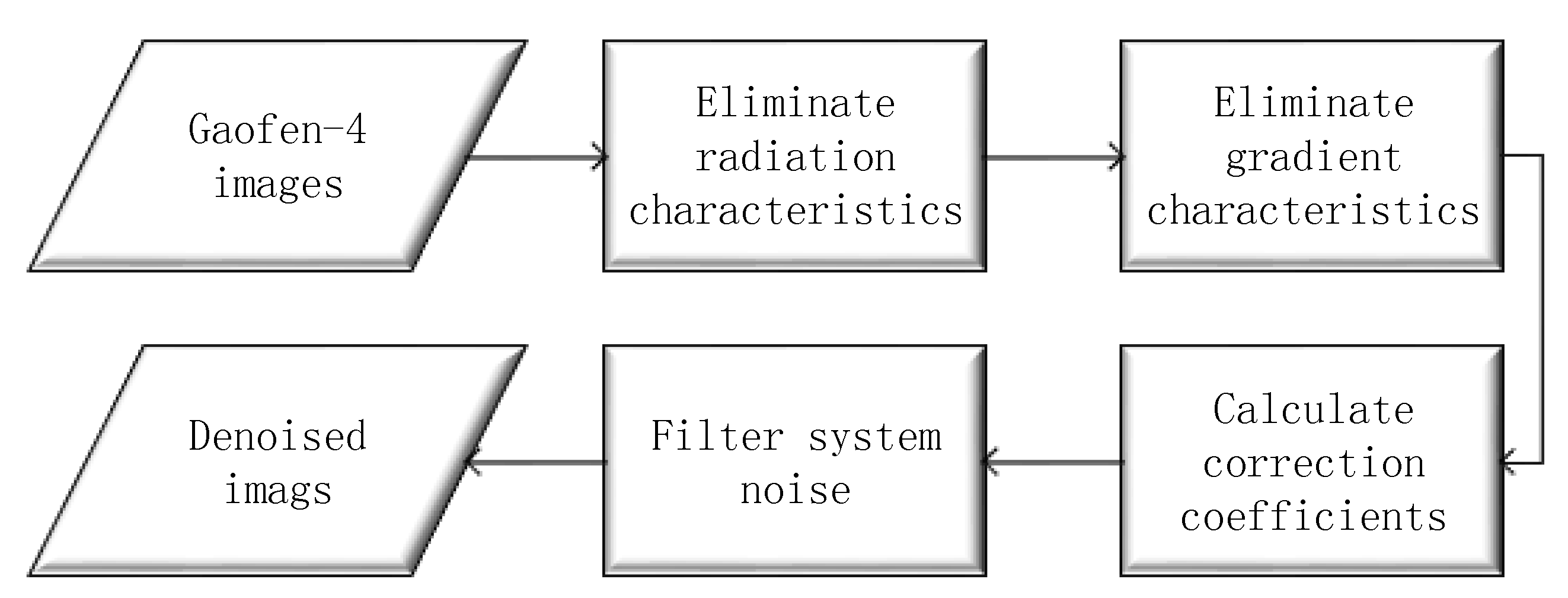
2.1. Principle of Gaofen-4 System Noise Removal

Gaofen-4 is equipped with an area array complementary metal–oxide semiconductor (CMOS) sensor and a mercury cadmium telluride (HgCdTe) sensor. The CMOS sensor is used to generate visible light and near-infrared (VNIR) images. VNIR images have five bands with a spatial resolution of 50 m. The HgCdTe sensor is used to generate medium-wave infrared (MIR) images with a spatial resolution of 400 m. Figure 1 shows the five bands of a Gaofen-4 VNIR image. It can be seen in Figure 1 that the fourth band (630–690 nm, red light) is the most serious band of noise pollution. Figure 2 shows the noise situation of four different VNIR images within band 4; all of the sub-figures are cut from same image location. It can be seen from Figure 2 that the noise locations are the same, and the noise intensities are similar. These phenomena indicate that the noise is systematic, rather than random.
The system noise of Gaofen-4 are mainly caused by the different responses of optical systems, the different responses of CCD detectors, broken detectors, dark currents in CCDs, and so on [20]. These factors will cause stripe noise in pushbroom satellites. However, as Gaofen-4 is equipped with an area array camera, these factors will cause point noise. Among these factors, the different responses of optical systems, the different responses of CCD detectors, and broken detectors will cause multiplicative noise; dark currents in CCDs will cause additive noise.
In general, these influencing factors should be filtered out in the relative radiometric correction. However, if the correction coefficients are not accurate enough or the satellite state changes, multiplicative and additive noise will remain in the images and become system noise. For a linear responsive sensor, the relative radiometric correction model can be described by Equation (1):
D N c = D N r B N G ,
where D N c is the corrected digital number (DN) value without system noise, D N r is the original DN value of the received data (Level-0 image), B is the offset value, and N G is the normalized gain value. The original DN value D N r was polluted by multiplicative noise and additive noise. The experimental data are all Level-1 images that have already been processed by relative radiometric correction in the data production stage. So, the DN value of a Level-1 image has changed, and can be described by Equation (2):
D N c , 1 = D N r B 1 N G 1 ,
where B 1 and N G 1 are the relative radiometric correction coefficients used in the data production stage, and D N c , 1 is the DN value of a Level-1 image. Equation (2) is substituted into Equation (1), and Equation (1) can be modified as:
D N c = ( D N c , 1 N G 1 + B 1 ) B N G = N G 1 N G D N c , 1 B B 1 N G = α D N c , 1 β .
Equation (3) is still a linear function, where α = N G 1 / N G is used to correct multiplicative noise and β = ( B B 1 ) / N G is used to correct additive noise. Multiplicative noise is the major factor of system noise, and additive noise is the secondary factor. In addition, the number of multiple images is small; it is difficult to calculate β accurately based on the least square method by such a small sample. Based on these considerations, we set β to 0, and α can be obtained by Equation (4):
α = D N c / D N c , 1 .
If the accurate α can be obtained, the system noise of Gaofen-4 can be filtered out. Therefore, the key to filtering out the Gaofen-4 system noise lies in simulating the corresponding noise-free image.
Pushbroom optical satellites are equipped with linear array CCD cameras. Linear array CCD cameras have a small number of detector cells, typically several thousands. Each column of the image is taken by same detector cell. With the accumulation of data, the response curve of each detector cell can be drawn and used for uniform correction. However, geostationary satellites are equipped with area array cameras. Area array cameras have up to hundreds of millions of detector cells, and every pixel in a picture is taken by a different detector cell. Even though the thousands of images are used for statistics, it is still not enough to describe the response curve of each detector cell. Therefore, traditional on-orbit radiometric calibration is ineffective for area array cameras, and the radiometric calibration coefficients are relatively inaccurate.
Suppose there are unlimited numbers of noise-free images, and the feature distribution of each image is irrelevant. As the number of multiple images increases, their superimposed image should tend to be uniform gradually. If system noise exists in multiple images, it will be highlighted in the superimposed image; then, random variables, such as radiation features, random noise, topography, and spatial information will be gradually eliminated. However, both prerequisites are not established in reality. First, the number of multiple images is limited. Second, the data contain many gaze images, repeated images, and overlapping images, which means there is a correlation between images. Therefore, these random variables cannot be completely eliminated, and become error terms. Among these random variables, the greatest influencing factors are the different radiation characteristics and gradient characteristics among the multiple images. If the radiation characteristics and gradient characteristics can be eliminated, the position and intensity of the system noise can be determined by multiple images of a small number, and the system noise can be removed easily.
Based on this idea, the main flow of system noise removal for the Gaofen-4 area array camera includes four steps: (1) eliminate the radiation characteristics, (2) eliminate the gradient characteristics, (3) calculate the correction coefficients, and (4) filter the system noise. The flow chart is as shown in Figure 3:

2.2. Elimination of Radiation Characteristics

The radiation characteristics of remote sensing images are affected by many factors, including light intensity, imaging angle, spectral range, and underlying surface type. Under the coupling of various factors, it is almost impossible to construct a complete and accurate model, and exclude each influencing factor one-by-one based on the constructed model. Therefore, we convert the original image into a texture image to eliminate most of the radiation characteristics and only retain gradient distribution and noises. The texture image is produced by Equation (5):
T ( i , j ) = I ( i , j ) I f ( i , j ) ,
where T is the texture image, I is the input image, I f is the blurred image processed by Gaussian filtering, and ( i , j ) are the image coordinates.
Figure 4 shows the radiation characteristics elimination result, where (a) is the original image, (b) is the corresponding blurred image, and (c) is the corresponding texture image. It can be seen from Figure 4 that snow, rocks, and shadows in the original image are easy to distinguish. However, in the texture image, the difference between rock and snow is basically eliminated, and the difference between shadows and normal features is also weakened. Noise can hardly be observed in the original image, but after the elimination of radiation characteristics, noise is greatly enhanced in the texture image.
Figure 5 is the spectra before and after filtering of a random pixel in the Gaofen-4 VNIR image. It can be seen from Figure 5 that the dispersion of the spectrum is greatly reduced by the elimination of the radiation characteristics. The spectrum before filtering is distributed between 0.3252 and 0.4785, and the spectrum after filtering is distributed between 0.9916 and 0.9996.
These phenomenon indicate that most of the spectral information and part of the structural information can be eliminated, and the noise intensity and image gradient information can be enhanced by the elimination of radiation characteristics.

2.3. Elimination of Gradient Characteristics

After the elimination of radiation characteristics, most of the spectral information has been removed, and most of the noise and gradient information has been preserved and enhanced. As the above description, system noise mainly comes from the different responses of CCD detectors, so their position, change direction, and range are fixed. Gradient information mainly comes from topography, and their position, change direction, and range are random. For multiple texture images, values with the same image coordinates can be constituted as an array. In this array, the distributed elements will be centrally influenced by system noise, and randomly influenced by gradient information. So, gradient information can be removed by rejecting gross errors in this array.
Since the elements distribution satisfies the Gaussian distribution and the number of samples is small (in this paper, the number of multiple images is 38), the Grubbs criterion is used to reject gross errors. The Grubbs criterion is suitable for rejecting gross errors from samples of a small number, and the determination of gross errors is independent of the mean and variance, and is easy to adjust and control [21]. The samples are written as y i ,   i = 1 , , N , and the observation data model can be constructed as Equation (6):
y i = μ + x i , x i N ( 0 , σ 2 ) .
The mean y ¯ and standard deviation σ ¯ of the samples are expressed as Equation (7):
{ y ¯ = 1 N i = 1 N y i σ ¯ = 1 N i = 1 N ( y y ¯ ) 2 .
Based on Shen et al. [21], a variable v can be established as Equation (8):
v = max | y i y ¯ | σ ,
and the variable can be transferred as Equation (9):
v N 2 N 1 v 2 t a ( N 2 ) .
Equation (9) is a t-distribution variable with N 2 degrees of freedom. Based on Shen et al. [21], when a test level α is given, t α ( N 2 ) can be calculated. The statistic v α , which is independent of both the mean and standard deviation, can be further calculated as Equation (10):
v α = t α N 1 N 2 t α 2 .
The statistic v α is the threshold that is used to determine if the elements are normal. If v > v α , the sample can be judged as a gross error and removed. In this paper, α is set to 90%, and the gross error obtained by each test is replaced by the mean of the samples. The results are shown in Figure 6, where (a) shows the compared arrays before and after removing the gross errors, (b) is a texture image, and (c) is the corresponding noise image. By comparing (b) and (c), it can be clearly seen that the high-gradient regions in the texture image, such as mountains and rivers, are filtered out basically, and only the noise points are revised in the noise image.

2.4. System Noise Removal

After eliminating radiation characteristics and gradient characteristics from the multiple images, the mean value of the array is used as the correction coefficient:
u ( i , j ) = M m = 1 M n m ( i , j ) ,
where u ( i , j ) is the correction coefficient, m is the order of multiple images, M is the number of multiple images, and n m ( i , j ) is the pixel of the corresponding noise image. The denoised image is obtained by Equation (12):
f ( i , j ) = f ( i , j ) × u ( i , j ) ,
where f is the denoised image and f is the original image.

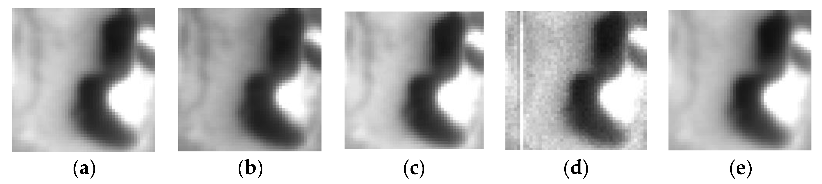
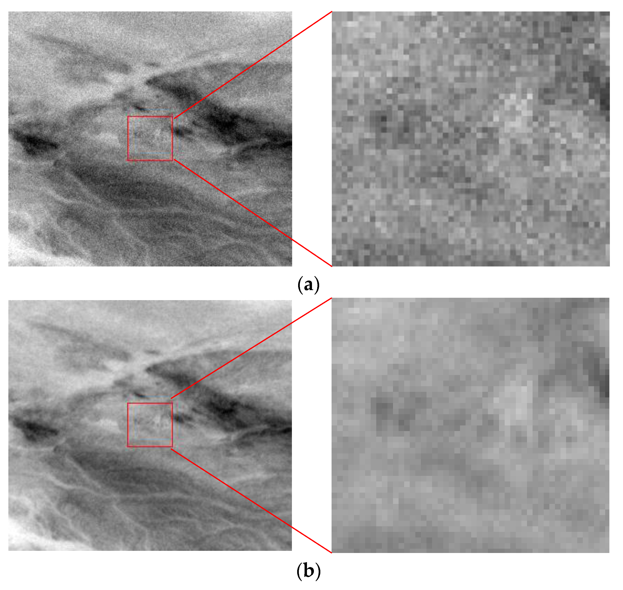
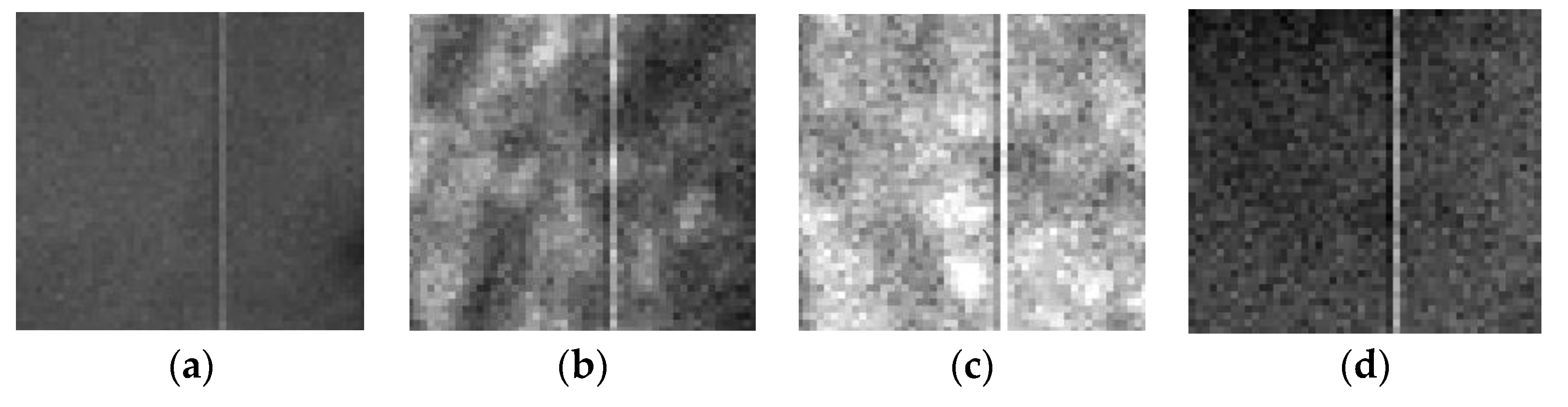
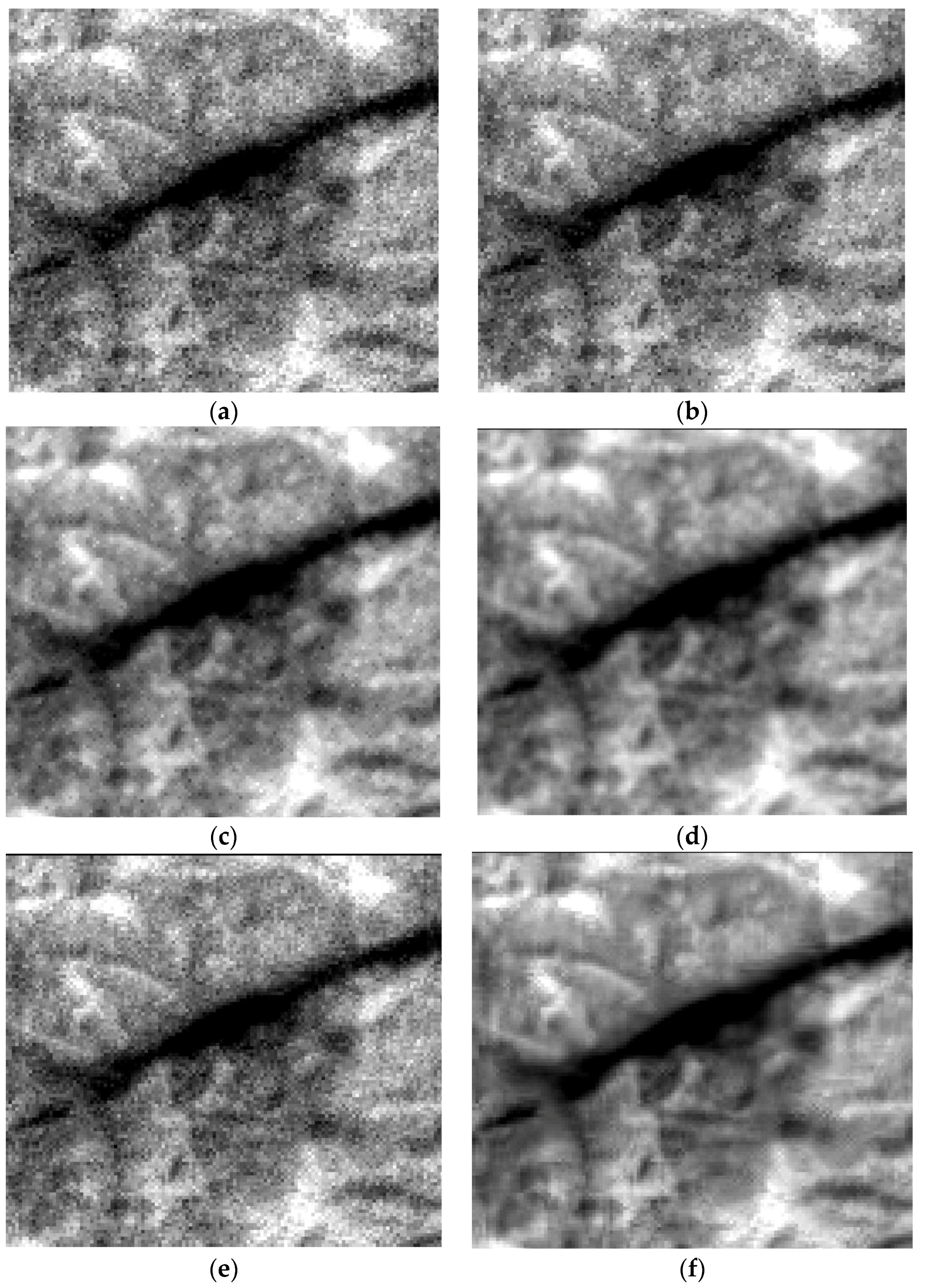
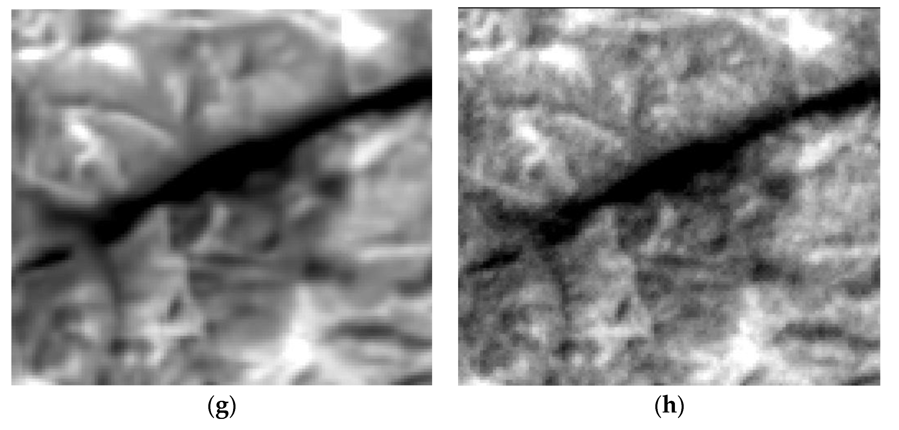
3. Results and Discussion

Thirty-eight Gaofen-4 VNIR images are selected as experiment data to calculate the correction coefficients, and one of them is selected as test data to check the denoising effect. The correction coefficient map of Gaofen-4 VNIR band 4 is shown in Figure 7, and the denoised result is shown in Figure 8.
Local sigma, BM3D, and the proposed method are separately applied to process the same Gaofen-4 VNIR image; the results are shown in Figure 9. The results are quantitatively evaluated by mean, standard deviation, and SNR, and the evaluation parameters are listed in Table 1. All of the evaluated parameters are calculated by the same test: one Gaofen-4 VNIR image. Due to the lack of a real noise-free image, SNR is measured by local standard deviation (LSD) [22]. The measurement procedure of LSD includes four steps: (1) calculate the mean value of the whole image, which is written as M ; (2) divide the image into small blocks with 10 × 10 pixels and calculate the standard deviation of all of the blocks; (3) set up 1000 bins with equal width within the minimum and maximum block standard deviation (the bin with the largest number, written as L S D max , is regarded as noise; and (4) calculate the results using Equation (13):
S N R = 20 lg ( M / L S D max )
The effective removal of image noise while preserving edge details and texture information is key to remote sensing image denoising. It can be seen from the results in Figure 9 that local sigma, BM3D, and the proposed method all have considerable denoising effects. With the increase of sigma value, the denoising ability of local sigma and BM3D are both improving, but their edge details and texture information retention effects are degenerating. When sigma is equal to three, local sigma has a similar SNR to the proposed method, which are 35.6646 dB and 35.8638 dB, respectively. However, it can be seen from comparing Figure 9d and Figure 9h that local sigma has lost more edge details and texture information than the proposed method. Figure 9e–g are all processed by BM3D. When sigma is equal to one, a lot of noise remained in Figure 9e. When sigma is equal to two, the noise intensity is decreasing rapidly in Figure 9f, but blocky traces are appearing, which seriously influences the visual effect. When sigma is equal to three, the noise is further denoising in Figure 9g, and the SNR is substantially increasing to 37.3435 dB. However, the image is overly smoothed at this time, and the similarity with the original image is seriously decreased, which has affected the practical application of the data. The proposed method removes system noise based on correlation to the time axis of the multiple images, not correlation of neighborhood. Therefore, the proposed method can remove system noise while retaining edge details and texture information effectively.

4. Conclusions

Gaofen-4 is equipped with an area array CMOS camera and an HgCdTe camera. When the relative radiometric calibration is not accurate enough or the satellite state changes, system point noise will appear in the images. Since the system noise is correlated to the time axis of the multiple images, we propose a denoising method based on this feature. Firstly, Gaussian filtering is used to eliminate the radiation characteristics in order to obtain multiple texture images. Secondly, the Grubs criterion is used to eliminate the gradient characteristics in order to obtain multiple noise images. Thirdly, the multiple noise images are used to calculate the correction coefficients. Finally, the correction coefficients are used to obtain the denoised image. Experiments show that this method can remove system noise from Gaofen-4 images effectively. In addition, this method is based on the correlation of the time axis to the multiple images, rather than correlation within the image neighborhood. So, it can keep edge details and texture information effectively.

Author Contributions

X.C. conceived and designed experiments; L.H. performed the experiments, analyzed the data and wrote paper.

Acknowledgments

The research was supported from the National Natural Science Foundation of China (No.41701527), the China Postdoctoral Science Foundation (2017M612509), the Fundamental Research Funds for the Central Universities (2042017kf0042). We are grateful to the data support from China Centre for Resources Satellite Data and Application, and the anonymous reviewers for their valuable suggestions.

Conflicts of Interest

The authors declare no conflict of interest.

References

  1. Mendenhall, J.A.; Lencioni, D.E.; Evans, J.B. Earth Observing-1 Advanced Land Imager: Radiometric Response Calibration; MIT/LL Project Report EO-1-3; Massachusetts Institute of Technology: Cambridge, MA, USA, 2000. [Google Scholar]
  2. Wang, M.; Cheng, Y.; Long, X.; Yang, B. On-Orbit Geometric Calibration Approach for High-Resolution Geostationary Optical Satellite GaoFen-4. Int. Arch. Photogramm. Remote Sens. Spat. Inf. Sci. 2016, 41, 389–394. [Google Scholar] [CrossRef]
  3. Gonzalez, R.C.; Woods, R.E. Digital Image Processing; Prentice Hall International: Englewood Cliffs, NJ, USA, 2005; Volume 28, pp. 484–486. [Google Scholar]
  4. Buades, A.; Coll, B.; Morel, J.M. A Review of Image Denoising Algorithms, with a New One. Siam J. Multiscale Model. Simul. 2005, 4, 490–530. [Google Scholar] [CrossRef]
  5. Dabov, K.; Foi, A.; Katkovnik, V.; Egiazarian, K. Image Denoising by Sparse 3-D Transform-Domain Collaborative Filtering. IEEE Trans. Image Process. 2007, 16, 2080–2095. [Google Scholar] [CrossRef] [PubMed]
  6. Witkin, A.P. Scale-space filtering. In Proceedings of the International Joint Conference on Artificial Intelligence, Karlsruhe, Germany, 8–12 August 1983; pp. 1019–1022. [Google Scholar]
  7. Perona, P.; Malik, J. Scale-Space and Edge Detection Using Anisotropic Diffusion. IEEE Trans. Pattern Anal. Mach. Intell. 1990, 12, 629–639. [Google Scholar] [CrossRef]
  8. Weickert, J. Theoretical Foundations of Anisotropic Diffusion in Image Processing. In Theoretical Foundations of Computer Vision; Springer: Vienna, Austria, 1996; pp. 221–236. [Google Scholar]
  9. Lerga, J.; Grbac, E.; Sucic, V. An ICI Based Algorithm for Fast Denoising of Video Signals. Automatika 2014, 55, 351–358. [Google Scholar] [CrossRef]
  10. Mandić, I.; Peić, H.; Lerga, J.; Štajduhar, I. Denoising of X-ray Images Using the Adaptive Algorithm Based on the LPA-RICI Algorithm. J. Imaging 2018, 4, 34. [Google Scholar] [CrossRef]
  11. Zorzi, M. An interpretation of the dual problem of the THREE-like approaches. Automatica 2015, 62, 87–92. [Google Scholar] [CrossRef]
  12. Ringh, A.; Karlsson, J.; Lindquist, A. Multidimensional Rational Covariance Extension with Applications to Spectral Estimation and Image Compression. Mathematics 2016, 306 Pt 1, 823–834. [Google Scholar] [CrossRef]
  13. Mallat, S.G. A Theory for Multiresolution Signal Decomposition: The Wavelet Representation. IEEE Trans. Pattern Anal. Mach. Intell. 1989, 11, 674–693. [Google Scholar] [CrossRef]
  14. Chipman, H.; Kolaczyk, E.; Mcculloch, R. Adaptive Bayesian Wavelet Shrinkage. J. Am. Stat. Assoc. 1997, 92, 1413–1421. [Google Scholar] [CrossRef]
  15. Moulin, P.; Liu, J. Analysis of multiresolution image denoising schemes using generalized Gaussian and complexity priors. IEEE Trans. Inf. Theory 2015, 45, 909–919. [Google Scholar] [CrossRef]
  16. Romberg, J.K.; Choi, H.; Baraniuk, R.G. Bayesian tree-structured image modeling using wavelet-domain hidden Markov models. IEEE Trans. Image Process. 2001, 10, 1056–1068. [Google Scholar] [CrossRef] [PubMed]
  17. Donoho, D.L. Ridge Functions and Orthonormal Ridgelets; Academic Press, Inc.: Cambridge, MA, USA, 2001. [Google Scholar]
  18. Emmanuel, J.C. Monoscale Ridgelets for the Representation of Images with Edges; Technical Report; Department of Statistics Stanford University: Stanford, CA, USA, 1999. [Google Scholar]
  19. Pennec, E.L.; Mallat, S. Image compression with geometrical wavelets. In Proceedings of the IEEE International Conference on Image Processing, Vancouver, BC, Canada, 10–13 September 2000; Volume 1, pp. 661–664. [Google Scholar]
  20. Duan, Y.; Zhang, L.; Yan, L.; Wu, T.; Liu, Y.; Tong, Q. Relative radiometric correction methods for remote sensing images and their applicability analysis. J. Remote Sens. 2014, 18, 597–617. [Google Scholar]
  21. Shen, Y.; Ran, Q.; Liu, Y. Application of Improved Grubbs’ Criterion to Estimation of Signal Detection Threshold. J. Harbin Inst. Technol. 1999, 31, 111–113. [Google Scholar]
  22. Gao, B.C. An operational method for estimating signal to noise ratios from data acquired with imaging spectrometers. Remote Sens. Environ. 1993, 43, 23–33. [Google Scholar] [CrossRef]
Figure 1. Noise situation of different Gaofen-4 visible light and near-infrared (VNIR) bands. (a) is band 1, (b) is band 2, (c) is band 3, (d) is band 4, and (e) is band 5.
Remotesensing 10 00759 g001
Figure 2. Noise situation of different VNIR images within band 4, where (ad) are all cut from the same image location.
Remotesensing 10 00759 g002
Figure 3. Flow chart of system noise removal for the Gaofen-4 area array camera.
Remotesensing 10 00759 g003
Figure 4. Result of radiation characteristics elimination. Where (a) is the original image; (b) is the corresponding blurred image processed by Gaussian filtering (sigma is 1, and kernel size is 5 × 5); and (c) is the corresponding texture image.
Remotesensing 10 00759 g004
Figure 5. Spectra before and after filtering of a random pixel in a Gaofen-4 VNIR image.
Remotesensing 10 00759 g005
Figure 6. Results of the gradient characteristics elimination, where (a) shows compared arrays before and after removing gross errors, and red dots are the gross errors; (b) is a texture image; and (c) is the corresponding noise image after the elimination of gradient characteristics.
Remotesensing 10 00759 g006
Figure 7. Correction coefficient of Gaofen-4 VNIR band 4.
Remotesensing 10 00759 g007
Figure 8. Result of Gaofen-4 system noise removal, where (a) is the original noisy image, and (b) is the corresponding denoised image processed by the proposed method.
Remotesensing 10 00759 g008
Figure 9. Processed results by different denoising methods, where (a) is the original noised image, (b) is the denoised image processed by local sigma whose sigma is equal to one, (c) is the denoised image processed by local sigma whose sigma is equal to two, (d) is the denoised image processed by local sigma whose sigma is equal to three, (e) is the denoised image processed by BM3D whose sigma is equal to one, (f) is the denoised image processed by BM3D whose sigma is equal to two, (g) is the denoised image processed by BM3D whose sigma is equal to three, and (h) is the denoised image processed by the proposed method.
Remotesensing 10 00759 g009aRemotesensing 10 00759 g009b
Table 1. Evaluation parameters of denoised images. BM3D: three-dimensional patch-based filtering method; SNR: signal-to-noise ratio.
MethodMeanStandard DeviationSNR (dB)
Original Image375.3394119.405527.4280
Local Sigma (sigma = 1)375.3642119.227428.6714
Local Sigma (sigma = 2)375.3359118.721432.7983
Local Sigma (sigma = 3)375.3507118.525035.6646
BM3D (sigma = 1)375.3382119.285928.2042
BM3D (sigma = 2)375.3355119.054931.0448
BM3D (sigma = 3)375.3325118.857137.3436
Proposed Method375.4924119.017035.8638

