Article

Metrology Assessment of the Accuracy of Precipitable Water Vapor Estimates from GPS Data Acquisition in Tropical Areas: The Tahiti Case

1
Geodesy Observatory of Tahiti, University of French Polynesia, Faa’a 98702, French Polynesia
2
Institute of Space Sciences, Shandong University, Weihai 264209, China
3
Department of Real Estate and Built Environment, National Taipei University, New Taipei 23741, Taiwan
*
Author to whom correspondence should be addressed.
Remote Sens. 2018, 10(5), 758; https://doi.org/10.3390/rs10050758
Submission received: 22 March 2018 / Revised: 5 May 2018 / Accepted: 11 May 2018 / Published: 15 May 2018
(This article belongs to the Special Issue Remote Sensing Water Cycle: Theory, Sensors, Data, and Applications)

Abstract

:
High precision Global Positioning System (GPS) receivers, with the advantages of all-weather work and low cost, are now widely used to routinely monitor precipitable water (PW) vapor. They are so successful that the progressive phasing out of the costly and sparse in situ radio soundings (RS) is now a certainty. Nevertheless, the sub-daily to annual monitoring of high levels of the PW by GPS receivers in the tropics and the equatorial area still needs to be asserted in terms of metrology accuracy. This is the subject of this paper, which focuses on a tropical site located in mid-ocean (Tahiti). The metrology assessment was divided into two steps. Firstly, a GPS internal assessment, with an in-house processing based on the Bernese GNSS Software Version 5.2 and a comparison with the Center for Orbit Determination in Europe (CODE) products. Secondly, an external assessment, with a comparison with RS PW estimates. In contrast with previous works that only used PW estimates from the Integrated Global Radiosonde Archive (IGRA) website, we estimated the RS PW from the balloon raw data. This is especially important in tropical areas, where IGRA estimates only consider balloon measurements taken below approximately 5500 m. We show that, in our case, this threshold is one of the main sources of bias between GPS and RS estimates, and that the formula used to translate the GPS zenith wet delays (ZWD) to PW estimates also needs to be revisited for high level water vapor contents in the atmosphere.

1. Introduction

Atmospheric water vapor plays an important role in atmospheric processes including atmospheric radiation balance, water cycles, the transfer of energy, and the formation of clouds and precipitation [1,2,3]. Water vapor is also the most abundant and a critical component of the greenhouse gases driving global weather and climate changes [4,5,6]. Integrated precipitable water vapor (IPWV, or PW for short) is the total water vapor contained in an air column from the Earth’s surface to the top of the atmosphere. About 45–65% of the PW is included from the surface to 850 hPa altitude (roughly 1500 m) and its distribution is highly variable in time and space [7,8]. Real-time and accurate estimates of characterization of the PW at high spatial and temporal resolution are now needed for severe weather forecasting and climate warming studies [9,10].
Many meteorological techniques that have been used for decades to retrieve PW, such as radiosondes, water vapor radiometer, and infrared sounders are expensive and may give poor data quality and poor spatial coverage [11,12,13]. Besides, these traditional techniques measure the PW distribution only at coarse scales. These limitations form the main source of error in short-term precipitation forecasts [14]. In contrast, PW estimates derived from Global Positioning System (GPS) measurements have been routinely done in the last twenty years with high internal repeatability, all-weather capability, and low cost [15,16]. The spatial resolution of PW by using GPS data depends on the number GPS receivers deployed on the Earth surfaces [17,18]. Nowadays, with the always increasing density of GPS sites, the application of ground-based GPS PW detection is strongly promoted in the meteorological field [19]. Many studies are focused on the PW estimates obtained from GPS technique. Ohtani et al. (2000) have investigated the accuracy and features of PW estimates obtained from Japanese GPS networks and compared them with radiosonde observations [20]. Kwon et al. (2008) have made a comparison between GPS PW estimates derived from a permanent ground-based GPS network on the Korean Peninsula and radiosonde measurements [21]. Choy et al. (2015) have compared PW derived from grounded-based GPS receiver with traditional radiosonde measurement in Australia [22].
GPS radio signals are delayed when they pass through the ionosphere (the upper part of the atmosphere) and the neutral atmosphere. Part of this propagation delay is caused by the atmospheric water vapor, which is mostly concentrated in the troposphere, and this delay can be estimated as a function of the temperature, pressure, and water vapor contents of the atmospheric layers [23,24]. It can be essentially reduced to the knowledge of the zenithal total delay (ZTD), itself divided into two components: zenithal hydrostatic delay (ZHD) and zenithal wet delay (non–hydrostatic) (ZWD) [25,26]. The GPS ZWD can be converted to a PW estimate by a conversion coefficient   Π , which is related to the weighted mean temperature of water vapor (Tm) [27,28,29]. A standard processing is to compute Tm, then Π and finally PW from ZTD minus ZHD. It is clear that, from a mathematical point of view, this standard processing defines an iterative procedure, as we need an a priori guess of the water vapor contents of the atmosphere to determine the PW estimate. In practice, Tm is expressed as a linear function of surface temperature (Ts).
The ultimate goal is to get the slope and intercept of this linear function almost site-independent. This linear relationship has been explored by many scientists, both globally and regionally, from an a priori knowledge of the water vapor contents of the atmosphere from radio soundings. In 1992, Bevis et al. [30] came up with T m = 70.2 + 0.72 × T s from the analysis of 8718 profiles of radiosonde launches at 13 stations in the US over two years. This relation has been widely used in North Hemisphere mid-latitude regions between 27°N and 65°N, and was revised in 1994 by Bevis et al. [31], from a nearly global distribution of about 250,000 radiosonde profiles. In 1998, Mendes et al. [32] proposed another linear Tm model by using about 32,500 radiosonde profiles over one year at 50 sites between 62°S and 83°N. A dedicated model is available for high latitudes [33]. Liou et al. [34], Bai [35], Wang et al. [36], Raju et al. [37], Emardson et al. [38] also established regional and global linear relationships between Tm and Ts [39,40,41,42].
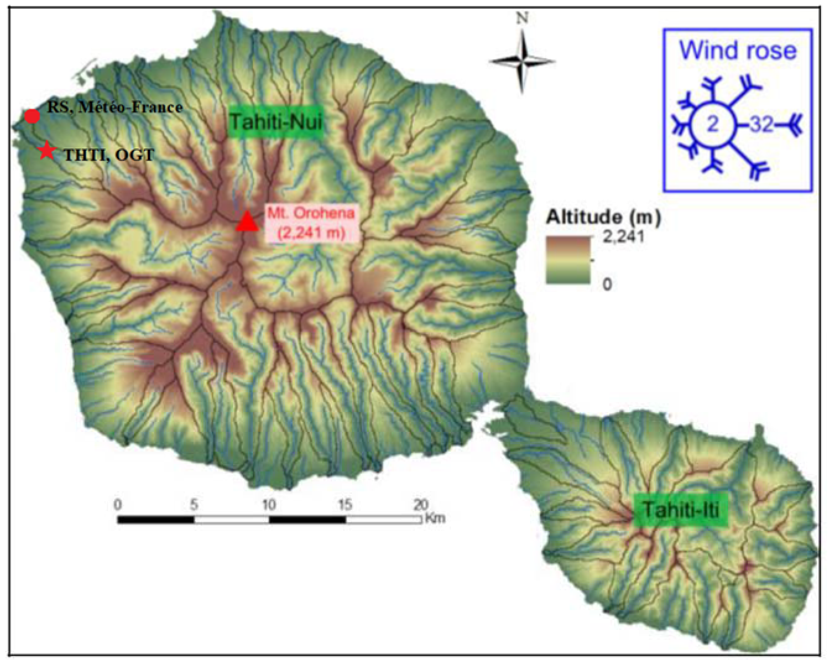
Of course, if we have an on-site good estimate of both the PW from an external source (essentially radio soundings, but this can be also absorption lines of water vapor in the atmosphere or radiometric observations), and ZWD from a collocated GPS receiver, then Π   and Tm can be directly derived. If, furthermore, we have a collocated weather station giving us Ts, then we can obtain by linear regression over a time series of Tm and Ts site-dependent values of the slope and intercept. This is basically the approach we applied in this paper, as we had the luxury to have a radio sounding station close to the Geodesy Observatory of Tahiti (OGT), with an International GNSS Service (IGS)-grade GPS receiver with weather data.
In this paper, the dataset and methodology are described in Section 2. The comparisons of GPS-derived results with the Center for Orbit Determination in Europe (CODE) products [43], as well as results obtained by using the Saastamoinen model are given in Section 3. In Section 4, we compare PW values downloaded from IGRA website and PW values computed from balloon raw data. The comparisons between our all-seasons Tm model and our season-specific Tm models with respect to the Bevis Tm model take place in Section 5. In Section 6, we compare and analyze the GPS-derived PW estimates based on our new Tm models with the corresponding RS PW estimates. Conclusions are presented in Section 7.

2. Study Area, Methodology and Datasets

2.1. The Study Area

The study area of this paper is the Tahiti island of French Polynesia, located on the tropical South Central Pacific Ocean (149°25′W, 17°40′S; Figure 1 [44]). The island of Tahiti (around 1000 km2) includes two volcanic systems that culminate at 2241 m (Tahiti-Nui), and at 1332 m in the southeast peninsula (Tahiti-Iti) [45]. The local climate, much more humid than in the other islands of French Polynesia [46], is governed by the South Pacific Convergence Zone (SPCZ) on the large scale, and by the topography of a high volcanic island on the orographic scale, including a fresh and dry period (“dry” season, with August being the driest month with 48 mm of precipitations) when southeast winds prevail (from May to October) and a warm and rainy period (“wet” season, the wettest month of which is January, peaking at 340 mm of rain in average) when northeast trade winds are predominant (from November to April) [47]. During the wet season, from November to April, significant land-slides and flash-floods are common, generating large property damages and casualties. For our data processing, we used the GPS data from the permanent IGS station (THTI) of the OGT and the radio soundings from the nearby (2 km) Météo-France weather station. Both locations (Figure 1) are in the suburbs of Tahiti capital city, Papeete.

2.2. GPS and Weather Data

The permanent GPS station THTI (IGS reference name) of the OGT (about 100 m altitude) consists of a TRIMBLE NETR8 receiver with an ASHTECH geodetic L1/L2 antenna. GPS satellite precise orbits and clocks as well as consistent Earth-rotation parameters provided by the Center for Orbit Determination in Europe (CODE), together with precise positioning point (PPP) approach under the Bernese GNSS Software Version 2, were used to estimate ZTD [43]. The software parameters are set, in all our processing, as follows: sampling rate is 300 s, elevation cut-off angle is 3 degrees, temporal resolution is 2 h and ionosphere correction is L3 free linear combination. We also considered the atmospheric loading and the ocean tidal loading corrections in the Bernese processing. In this study, we used the hydrostatic Vienna mapping function (VMF1) [48], with input data from the European Center for Medium-Range Weather Forecasts (ECMWF), as the a priori ZHD model, with wet and dry VMF1 mapping function [49,50].
The GPS-derived ZTD comprises ZHD and ZWD, as shown in Equation (1):
Z T D = Z H D + Z W D
And, the relationship between ZWD and PW [27] can be expressed as:
P W = Π · Z W D
where
Π = 10 6 ρ · R v ( k 3 T m + k 2 )
and
T m = P v T d z P v T 2 d z
where ρ = 1000   kg / m 3   is the density of liquid water, R v = 461.495   J / Kg · K is the specific gas constant of water vapor, k 2 = 22.1   K / mb and k 3 = 3.739 · 10 5   K 2 / mb are physical constants. The coefficient Π is a conversion coefficient, in practice a mean value of about 0.15 ± 20%. Pv is the partial pressure of water vapor, T is the absolute temperature in Kelvin. Both Pv and T are pointwise values taken along the vertical column. In our case, Tm (in Kelvin) is linearly related to Ts, as given by Equation (5):
T m = a + b · T s
where a and b are the intercept and slope of this linear function.
The estimation of ZWD (Equation (1)) from GPS-derived ZTD essentially requires empirical models of the ZHD, like the Saastamoinen model, the accuracy of which is approximately 1–2 mm [51] for the ZHD estimation.
The Saastamoinen model is defined as:
Z H D = 2.2768 P s f ( λ , H )
where f ( λ , Η ) = 1 0.00266 · cos ( 2 λ ) 0.00028 · H , λ (rad) is the station latitude, H (km) is the geoid height in kilometers and Ps (hPa) is the surface pressure. For sub-diurnal studies of the water vapor contents from GNSS data, the sampling rate is usually 30 min or less, but in our case, as we were primarily interested in comparisons with the CODE products and radio soundings in regard to a seasonal time frame, a 2 h sampling is perfectly adapted.
In our study, the meteorological parameters (the surface pressure Ps and the surface temperature Ts) are from the gridded VMF1 (vmf1_g) data of the European Center for Medium Range Weather Forecasts (ECMWF, http://ggosatm.hg.tuwien.ac.at). They are based on a 2 ° × 2.5 ° global grid (2 degrees sampling from North to South and 2.5 degrees sampling from West to East), with a 6-hourly temporal resolution (at 0h00, 6h00, 12h00 and 18h00 UTC). These gridded data have facilitated some high accuracy geodetic applications over the past years [52]. To validate the vmf1_g, we compared the vmf1_g downloaded values to the corresponding values measured at the OGT site (weather station of the TAH1 GPS receiver, ftp://garner.ucsd.edu, collocated within a few meters from THTI).
To validate the accuracy of the estimates of the ZTD and ZWD computed through the Bernese software with the VMF1 mapping function, we compared them with the CODE troposphere products (ftp://ftp.unibe.aiub.ch) and with the ZTD and ZWD derived from the Saastamoinen model (SAAS ZWD) relative to the THTI station with on-site weather data. The CODE products are also calculated by using the Bernese 5.2 software, but with a relative positioning technique and ionosphere-free linear combination of L1 and L2, their sampling rate is 180 s. The a priori ZHD model and mapping functions and the other processing parameters of CODE troposphere products are, from their documentation [43], the same as the ones used for our GPS data processing.

2.3. Radiosonde Level 1 and Level 2 Data

As mentioned above, a radio sounding balloon station is located close to our THTI GPS receiver in Tahiti Island (Figure 1). The horizontal distance is about 2 km and the height difference is around 100 m [44]. Balloons are launched once a day (0:00 UT) or twice a day (0:00 and 23:00 UT or 0:00 and 12:00 UT). They include pressure, temperature, relative humidity velocity and wind direction sensors.
In our study, the RS PW values coming from this station are relative to two different processing levels of the same raw data. The level 1 PW values are retrieved from the Integrated Global Radiosonde Archive (IGRA: ftp://ftp.ncdc.noaa.gov/) managed by the National Oceanic and Atmospheric Administration (NOAA) [53,54]. This archive is highly compressed, based on the characteristic points of data profiles, from the surface to 500 hPa (about 5500 m). This geopotential altitude is often referred to as a steering level, because the weather systems beneath, near to the Earth’s surface, roughly move in the same direction as the winds at the 500 hPa level. We computed in our observatory the level 2 data from the 1-second balloon raw data that we retrieved from the Météo-France in-house archive. They consist of pressure, temperature, relative humidity and GPS positioning from the surface to the maximum altitude of the balloon, i.e., 25,500 m (around 1 h 20 min of ascent). When the balloon explodes, its lateral drift can reach up to 20 to 50 km, depending on the direction and intensity of the wind. Macpherson [55] found that we can neglect the space-time drift of radiosonde balloons during their ascent for mesoscale numerical weather prediction models. Specifically, while the impact of balloon drift can indeed be detected, it is small compared with the impact from the observation when assimilated into the numerical weather prediction model with neglect of balloon drift. We computed these level 2 PW values by applying the procedure outlined in [8,56] as:
P W = 1 ρ ρ w d h
with
ρ w = R H 100 · R v · T · e s
and
e s = f · 6.1121 · e ( 18.729 t 227.3 ) · t t + 257.87
where h is the geopotential altitude, ρ   is the density of liquid water, ρ w   is the density of water vapor, R H   is the relative humidity, R v   is the specific gas constant of water vapor, T = t + 273.15 , t   is the surface temperature in Celsius, e s   is the saturation vapor pressure in hPa, f = 1.0007 + 3.46 · P s · 10 6   is the enhancement factor, and P s is the surface water vapor pressure.

2.4. Construction of the Tm Models

As we have two series of GPS (ZWD_GPS) and RS (PW_RS) data coming side by side, we can construct time series of “instantaneous” Π   according to Equation (10), which is the reversed version of Equation (2):
P W _ R S Z W D _ G P S = Π
Then the time series of Π values can be linearly fitted with respect to the ground temperature Ts for a given duration of time (Equation (5)). We can then distinguish many subcases, depending on how PW_RS is exactly computed (choice of mapping function and local tailoring of the chosen mapping function, including temperature and pressure) and which level (1 or 2) is chosen for PW_RS. We can also distinguish between wet and dry seasons for the fit to the local ground temperature Ts.
For the meteorological parameters entering the mapping functions, we used the data from the VMF1/ECWMF archive and local data from the nearby local station GPS station TAH1 (which also provides the Ts time series).

2.5. Definitions

In the following sections, we will use the usual statistical tools of Bias, root mean square (RMS) and standard deviation (STD) between two time series. To avoid any misunderstanding, we precise the definitions here:
B i a s = 1 n i = 1 n ( S ( i ) R ( i ) )
S T D = 1 n i = 1 n ( ( S ( i ) R ( i ) ) B i a s ) 2
R M S = 1 n i = 1 n ( S ( i ) R ( i ) ) 2
where i = 1 , 2 , 3 , , n . is the number of data point, S and R represent any time series with the same time sampling, with R taken as a reference.
We will also do time averaging, in the form [45]:
S ¯ [ i ] = j = 1 n S [ j ] * v i j j = 1 n v i j
where S [ j ] is the value of S corresponding to the j-th epoch. We will always use an averaging over one month, t = MJD (Modified Julian Day), Δ t = t j t i , i , j = 1 , 2 , 3 , , n , if | Δ t | > T , we set v i j = 0 , otherwise,   v i j = 1 .

3. Comparisons of ZTD and ZWD Values from Our GPS Data Processing, CODE Products and Saastamoinen Model

3.1. Comparisons of Our GPS-Derived ZTD and ZWD Values with CODE Products

In a first step, we compared home-brew ZTD and ZWD estimates based on our Local VMF1 Processing (LVP) over three years (2011–2013) for the THTI station with the estimates from the CODE products relative to the same station, to detect any gross differences. For this purpose, we employed the Bernese 5.2 software with the hydrostatic VMF1/ECMWF model (VMF1 dry and wet mapping function). Nowadays, the VMF1 mapping function is widely seen as the mapping function providing, from a global point of view, the most accurate and reliable geodetic results [50]. It should be noted that we used the PPP approach, but that CODE products, also processed with the help of the Bernese 5.2 software and the VMF1 dry and wet mapping function, are using a relative positioning approach and an ionosphere-free linear combination of L1 and L2, with a sampling rate of 180 s.
Figure 2 and Table 1 summarize the results. The distribution of the differences between our LVP processing and the CODE products, both for the ZTD and ZWD estimates are clearly close to a Gaussian distribution with no appreciable bias and an RMS of 6 mm. We can then consider the two processing as consistent. The ZWD differences are probably coming from the choice of PPP versus relative positioning, and the different ionosphere-free linear combination and sampling rate settings. The ZTD differences are caused by the ZWD differences.
Besides, we noted that some El Niño events took place from 2014 to 2016 [46]. To validate our LVP ZTD and ZWD, we also made comparisons between our results and CODE products during these three years. Table 1 shows good agreement between our LVP ZTD and ZWD and CODE products. The bias between the ZTD and ZWD time series is respectively 0.34 mm and 0.50 mm and RMS and STD are all about 7 mm. The above discussions reflect that the results of our LVP ZTD and ZWD meet the accuracy requirement and can be used in the following data processing.

3.2. Comparison of Our SAAS ZWD with Our LVP ZWD and CODE ZWD

We did an estimation of the ZWD (called here SAAS ZWD) over the period of 2014–2016 by using the LVP ZTD from the Bernese 5.2 data processing and the Saastamoinen model [51], fed with pressure data from the vmf1_g, because the weather station of the TAH1 GPS receiver stopped working in 2015. Figure 3a,b and Table 2 summarize the results with a comparison with the ZWD estimates from the previous section (VMF1 mapping functions) and CODE products.
Table 1 and Table 2 indicate that all the processing (in-house VMF1 and on Saastamoinen) give essentially the same results (internal consistency), paving the way to a comparison of our LVP ZWD and their derived PW values with the RS PW values.

4. Comparison of Level 1 RS PW Values with Level 2 RS PW Values

We will now assert the internal consistency of RS data. For this purpose, we recalculate in this section the local PW data from raw balloon measurements (level 2 RS PW in the jargon of the meteorological community, that we split into two subsets: a/level 2-A RS PW values, from the surface to the 500 hPa level and b/level 2-B RS PW values from the surface to the maximum altitude of the balloon, roughly 25,500 m in the mean) and make a comparison with the corresponding archived PW data from the IGRA website (level 1 RS PW). We emphasize that the IGRA archive contains only the level 1 data, that are highly compressed by the archive builders, which only retained the “characteristics” points of the raw data profiles, in the sense that the behavior of the data is identified as linear between these points. Besides, the archive builders limited, by construction, the maximum altitude of the data used to compute the archive from the surface to the 500 hPa level. In other words, they assumed that no PW was present beyond this level, or that this PW is irrelevant for meteorological studies. Still, in other words, the level 1 data should be, at least, consistent with the level 2-A if the compression algorithm is correct, and consistent with level 2-B if the assumption that no PW is present beyond the 500 hPa level is correct. This is the topic of the following sub-sections.

4.1. Comparison of Level 1 RS PW Values with Level 2-A RS PW Values (from the Surface to the 500 hPa Level)

In this section, we analyze and compare the reconstructed and archived PW from the surface to 500 hPa altitude with the level 2-A RS PW values we computed from the balloon raw data. We only used the 2014–2016 period, as instrumentation was changed at the end of 2013 at the Météo-France weather station. We recall that level 1 RS PW values are relative to the surface to the 500 hPa level and were downloaded from the IGRA archive, and that level 2-B RS PW values are relative to the surface to the maximum altitude of the balloon, far over the tropopause. We recomputed the level 2 data from raw balloon data stored in Météo-France archive, but here only up to the 500 hPa level (so-called level 2-A) to assert the reliability of archived level 1 PW data with regard to this threshold altitude.
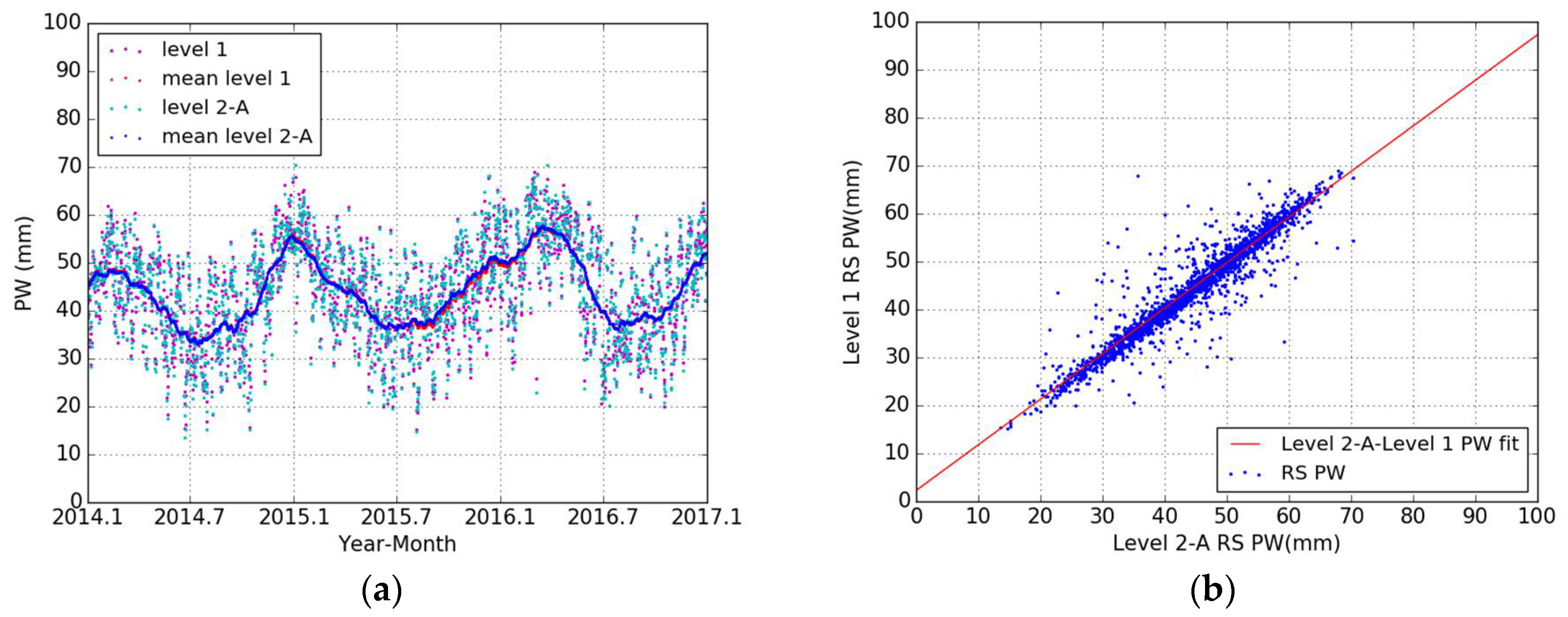
Figure 4a shows the time series of level 1 RS PW and level 2-A RS PW and the corresponding monthly averaged values from 2014 to 2017. Figure 4b shows the relationship between level 1 RS PW and level 2-A RS PW, and their least-squares fit is: level_1 = 0.95 × level_2-A − 2.29, with R2 = 94.62%. Figure 4a and Table 3 show clearly that the two sets of values are consistent, with a small bias (−0.10 mm) and an RMS of 1.30 mm. this means that the compression algorithm used to save space on the IGRA archive (storage of characteristic points of data profiles) is working, but with only a 95% “performance” in our particular case.

4.2. Comparison of Level 2-A RS PW Values (from the Surface to the 500 hPa Level) with Level 2-B RS PW Values (from the Surface to the Maximum Altitude of the Balloon)

Now, we compare the same sets of level 2-A data taken from the ground to 5500 m with regard to level 2-B data, i.e., data taken from the ground to the maximum altitude of the balloon (over 25,500 m). 
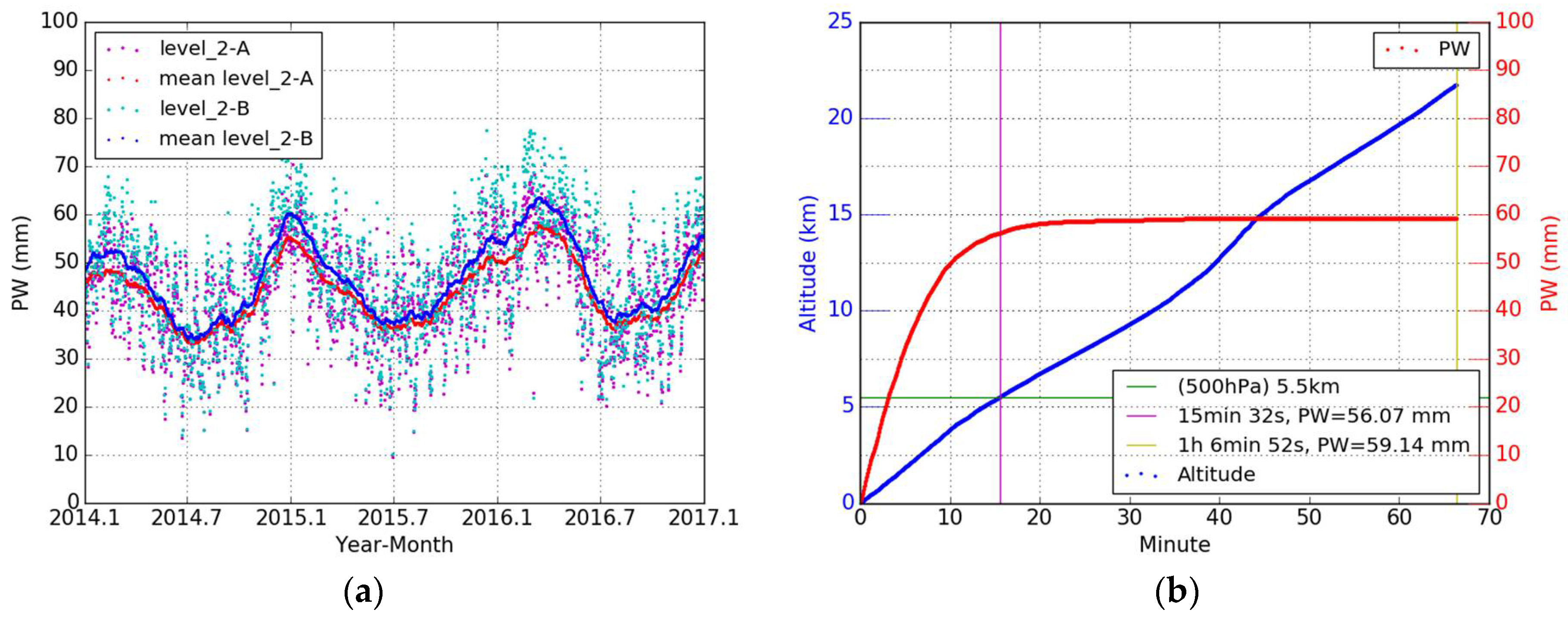
Figure 5a map level-2A versus level 2-B RS PW values over three years, with basically two launches of balloons per day. The level 2-B RS PW values are always larger than the corresponding level 2-A values. The statistic of their differences can be found in Table 4. The bias is 2.75 mm, the STD is 2.32 mm and the RMS is 3.60 mm. In order to better understand the relationship between the balloon altitude and the PW, we map in Figure 5b the level 2 data from a characteristic balloon launch at the Météo-France site, close to our observatory. The balloon reaches its maximum altitude, quasi-linearly with time, in about one hour. It is also clear from Figure 5b that the PW contents, integrated from the surface to the current altitude of the balloon also reaches a horizontal asymptote, and that this asymptote is pretty close, but does not correspond, to the 500 hPa level. About 95% of the maximum value of the PW is acquired after 15 min of ascent, and the last 5% in the remaining part of the ascent.
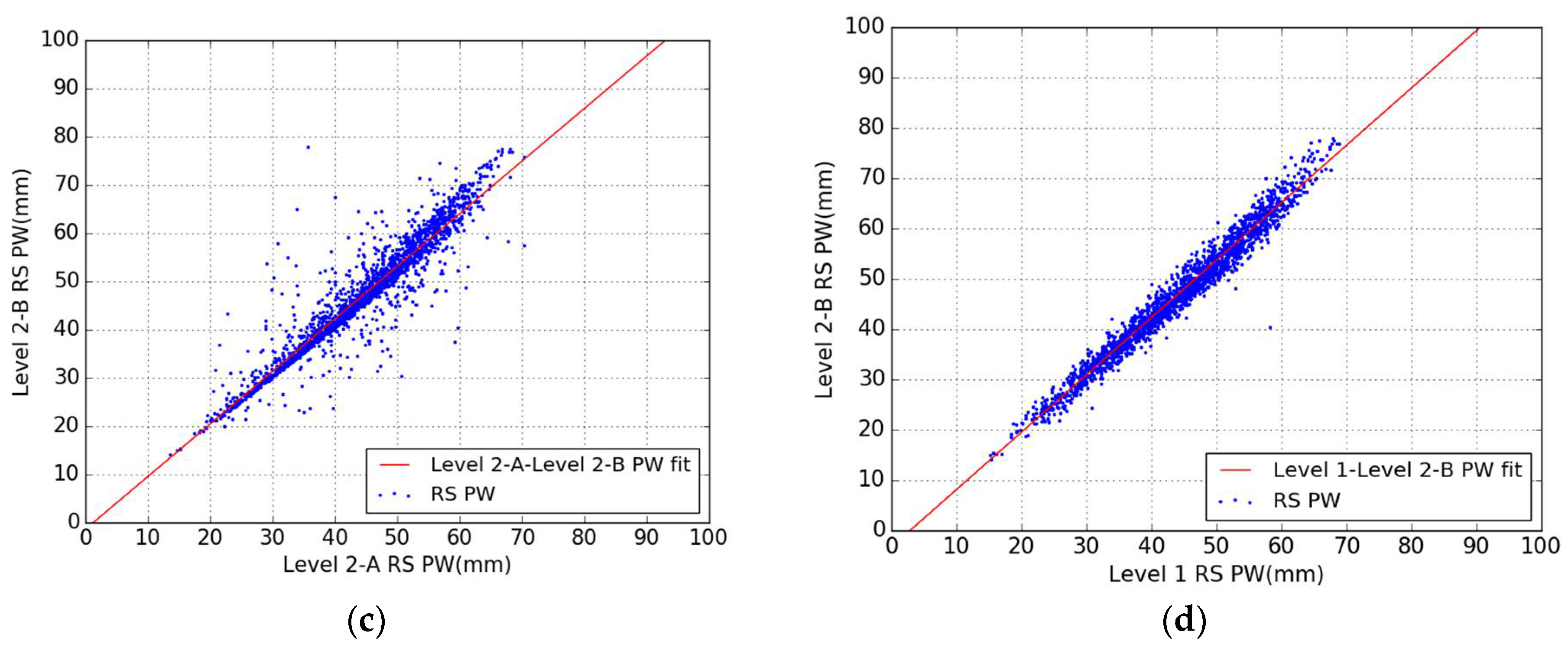
Figure 5c shows the relationship between level 2-A RS PW values and level 2-B RS PW values. Their least-squares linear fit is: level_2_B = 1.09 × level_2-A − 1.35, with R2 = 94.46%. Figure 5d shows the relationship between level 1 RS PW values and level 2-A RS PW values, and their least-squares linear fit is: level_2-B = 1.14 × level_1 − 3.29, R2 = 98.46%. Figure 5c and its linear fit indicates that, in the mean, the level 2-A values, in our case, underestimate the PW by about 9% with respect to the level 2-B values. One can argue that this difference is caused by the balloon lateral drift that can reach tens of kilometers when the balloon bursts. But the direction of the drift is highly variable as a function of the wind conditions during the balloon ascent, and this drift is essentially the cause of the scatter of the data points (about 2000 balloon launches) in Figure 5c. Therefore, our conclusion is still valid, in a certain sense. In Figure 5d we did the comparison between and level 2-B. The conclusion is the same, but in this case we add the “noise” coming from the compression algorithm used to build the level 1 data. We emphasize that all these conclusions are only relative to our site, which presents high values of the PW in the atmosphere, up to 60 mm, and sometimes even more. The level of 500 hPa was fixed decades ago by meteorologists for weather forecasting in temperate areas, and it is simply too low for tropical areas, contrary to the opinion of [57]. In tropical and equatorial areas, the water vapor layer reaches higher altitudes than in mid-latitudes areas, and up to 8 km in appreciable quantities [58].

5. All-Seasons Tm Model, Dry and Wet Season-Specific Tm Models for Our Site

5.1. Comparison of the Estimates of Our Tm Model, Bevies Tm Model and vmf1_g

The linear relationship T m = 70.2 + 0.72 × T s between Tm and Ts has been proposed by Bevis in 1992 [30], and is now used worldwide, thanks to its simplicity. Nevertheless, in 1997 Ross and Rosenfeld [59] found that this relationship weakens in the equatorial region and becomes even weaker in summer than in winter. It is clear from Figure 6 that the Tm values that we derived by applying Equation (10) differs greatly from the Bevis et al. estimates. Therefore, we decided to fit in our case local linear relationships, keeping in mind that the range of variations of our local ground temperature Ts is much smaller (8 K) than the range found in the Bevis et al. model (80 K).
In Figure 6a, we made a comparison among Tm estimates (Bevis et al. Tm, vmf1_g Tm and our Tm estimate from Equation (10)) over three years, from 2014 to 2016. The vmf1_g Tm estimate is calculated by using Equation (4) based on a 2 ° × 2.5 °   global grid with 6-hourly temporal spacing [48]. It is clear from Figure 6 that our Tm estimate shows an increasing uptrend with regard to the Bevis et al. and vmf1_g models, which exhibits much lower values and are almost equivalents. Figure 7 shows that the relationship between Tm and Ts in our case is still a linear one, albeit it is more “fuzzy” than in the work of Bevis et al., and that it also depends weakly on the season (dry or wet).
Table 5 shows the parameters (intercept and slope) of the linear least-squares fit to our LVP Tm corresponding to Figure 7. We applied the usual 3-sigma rejection rule for the rare outliers.
A Quantile-Quantile (QQ) plot of the residuals [60] indicates that no remaining structure can be found in the residuals of the fits in Figure 8, except maybe at the ends of the QQ line (see Section 6.2, Figure 12, and conclusions in Section 7).

5.2. Comparison of Mean LVP PW Based on the Local all Seasons Tm Model and Local Season-Specific Tm Models

Figure 9a shows the comparison of our monthly averaged values of LVP PW based on all-seasons Tm model and season-specific (dry and wet) Tm models. The consistency is pretty good, but it is also clear in Figure 9b that the use of separate dry and wet Tm models introduces discontinuities. During the dry season (from May to October), the mean PW differences between our LVP PW estimates computed with the all-seasons linear fit and our LVP PW estimates computed by distinguishing the dry and wet seasons (a linear fit per season) are a little bit closer to zero than the corresponding differences in the wet season (from November to April) (Figure 9b). It reflects the fact that the accuracy of PW estimates based on the wet season-specific Tm model is very close to the accuracy given by using the all-seasons specific Tm model. The LVP PW values derived by using the dry-season-specific Tm model seems to be not so good. This is may be related to the fact that during the dry season (less cloudy), the larger solar radiation heating of the humidity sensor may have caused larger biases [34].

6. Comparison of LVP PW Values with the Level 2-B RS PW Values

6.1. Comparison of LVP PW Based on Season-Specific Tm Model with Level 2-B RS PW Values

In order to test the accuracy of the PW estimates based on our new Tm models, we made a comparison between our LVP PW estimates based on our dry and wet season-specific Tm models and level 2-B RS PW values (from the surface to the maximum altitude of the balloon) from 2014 to 2016 (Figure 10a). We can see the consistency is good. Figure 10b shows that the PW differences are close to a Gaussian distribution with no appreciable bias (0.14 mm), an RMS of 3.29 mm and an STD of 3.29 mm, slightly biased toward positive differences (Table 6).

6.2. Comparison of Our LVP PW Values Based on Our all Seasons Tm Model with Level 2-B RS PW Values

Figure 11a shows the comparison of LVP PW estimates based on the all-seasons specific Tm model with the level 2-B RS PW estimates for the 2014–2016 period. We can see that their consistency is pretty good. Figure 11b shows that the PW differences are clearly close to a Gaussian distribution with no appreciable bias (0.04 mm), an RMS of 4.29 mm and an STD of 4.29 mm (Table 7). In term of bias, our all-seasons Tm model is better than our season-specific Tm model, but it is worse in terms of variance and extreme values.
We also made a comparison of our monthly averaged LVP PW values based on our all-seasons Tm model and season-specific (dry and wet) Tm models with the monthly averaged values of level 2-B RS PW from 2014 to 2016 (Figure 12a). The consistency is good (Figure 12a), but the differences (Figure 12b), albeit centered around zero, clearly indicate that a seasonal signal is still at play (see Figure 8b). It further reflects that the accuracy of our PW estimates based on our wet season-specific Tm model is better than the PW estimates based on our dry season-specific Tm model (Figure 9b), and in this case the all-seasons Tm model is a good choice to estimate the LVP PW values during the dry season.
From the above comparisons of our LVP PW values with level 2-B RS PW values, we can conclude that our Tm models according to the all-seasons, dry season and wet season are all reliable for accurate PW estimation in the tropical region of Tahiti. It further reflects that in our case the 500 hPa (5500 m) threshold is one of the main sources of bias between GPS PW and RS PW estimates.

6.3. Correlation of the Time Series of PW with the Fluctuations of Pressure and Temperature

We will now consider the correlations of our LVP PW estimates with weather data. We have two sources of weather data (temperature and pressure): The local TAH1 weather station (collocated with the THTI station), but, unfortunately, this weather station was stopped in mid-2015 and replaced by a new one by the end of 2017. The second one is the gridded VMF1 (vmf1_g) files (ECMWF grid weather data).
Figure 13a,c shows the comparison between the surface pressure and temperature downloaded from the gridded VMF1 files and the ones recorded at the TAH1 weather station, from 2011 to 2014. We note that the monthly averaged values of TAH1 recorded pressure and temperature is always higher than the vmf1_g values by 0.46 hPa and 0.73 K (Table 8). The vmf1_g documentation states that their records are relative to the site, and provides the station orthometric height. The observed bias of 0.46 hPa and 0.73 K may be due therefore to an instrumental bias on the sensor of the TAH1 weather station, but it is more likely related to how exactly the vmf1_g estimates are computed, and to the complex interactions between the lower atmosphere and the orography of the Tahiti Island. It cannot be due to the 100 m elevation of the station, as in this case the bias should have had the opposite value. According to these comparisons (Figure 13a,c and Table 8), we think that the surface pressure and temperature from gridded VMF1 files (ECMWF grid weather data) are reliable. Figure 13b,d shows the fluctuations of surface pressure and temperature downloaded from the gridded VMF1 files from 2014 to 2016. We used these surface pressure and temperature to calculate our ZHD values with regard to the Saastamoinen model (Equation (6)) and to model our new linear relationships (Equation (5)) between Tm and Ts for estimating the GPS PW values in Tahiti.
The variations of our mean LVP PW estimates (Figure 12a) are very clearly anti-correlated with the pressure variations (Figure 13a) and weakly correlated with the temperature variations (Figure 13c). This indicates that the culprit is probably the gridded VMF1 files (ECMWF grid weather data) that over-smooths the pressure and temperature that are entered in the VMF1 functions with respect to the true local values, and maybe, for high PW values, over-smooths the conversion factor Π of the Equation (3).

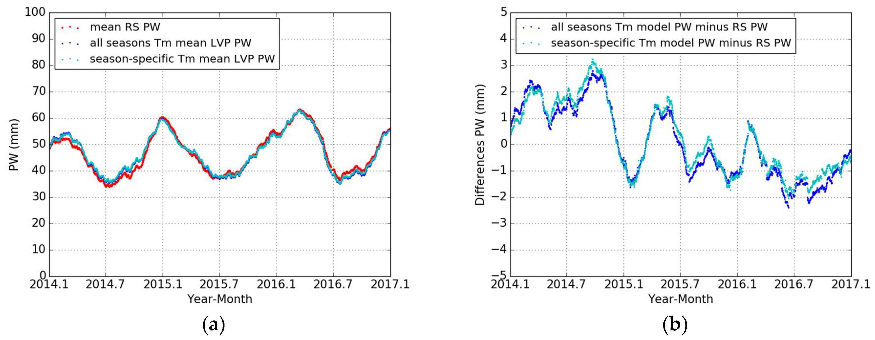
7. Conclusions and Outlook

In this research, we investigated, from a metrological point of view, the reliable retrieval of Integrated Precipitable Water Vapor (IPWV, or PW for short), from GPS data, in the tropical island of Tahiti. For this purpose, we did a cross-check between our GPS-derived estimates with the radio soundings data estimates from a nearby site, but also checked the internal consistency of the radio soundings estimates and of the GPS data estimates, in contrast to many studies that assume that the radio sounding data taken from the IGRA archive are “the” reference. In a first step, we checked the internal consistency of the modeling of the ZTD and ZWD estimates from our GPS data processing with respect to the CODE products and the Saastamoinen model. In a second step, we asserted the internal reliability of RS data. The first dataset we used, in this second step, is the archived PW data from the IGRA website (level 1 RS PW from the surface to the 500 hPa level). The second dataset, from the Météo-France archive, is the PW data from raw balloon measurements close to our site, sub-divided into two subsets: a/level 2-A RS PW, from the surface to the 500 hPa level and b/level 2-B RS PW from the surface to the maximum altitude of the balloon. Our analysis clearly indicates that the assumption of taking the IGRA archive as a reference can lead to an underestimation of the water vapor presents in the atmosphere in tropical areas (up to 9% in our case), and that only the RS level 2-B can be compared with the GPS-derived estimates in a consistent way. In a third step, we developed new models of the mean temperature Tm of the atmosphere with regard to its water vapor contents, based on a combination of level 2-B RS PW values and GPS ZWD values over Tahiti. The new Tm models based on all-seasons and different seasons (dry and wet) were derived by using meteorological data from the gridded VMF1 files. The results show that our all seasons Tm model and season-specific (dry and wet) Tm models are more reliable in our site (Tahiti) than the Bevis et al. model. In a fourth and last step, we compared our GPS PW estimates based on our new Tm models with level 2-B RS PW values. The results show that the PW derived with a “good” Tm model from GPS data is highly accurate, and as a final consequence confirms that the threshold of 500 hPa (5500 m) is the main source of bias between the GPS PW estimates and RS PW estimates taken from the IGRA archive in tropical areas.
Historically, the algorithms that are now widely employed to derive PW estimates from GNSS propagation delays can be traced down to the works of Owens in 1967 [61] on the optical refractive index of air, then Thayer in 1974 [62] on improved formulas, followed by Davis et al. in 1985 [27] who introduced the concept of the mean temperature Tm of the atmosphere with respect to its water vapor contents. The last essential brick to the edifice was laid down by Bevis et al. in 1992 [30] in the form of a linear relationship from the surface temperature Ts at the GNSS receiver site to the mean temperature Tm of the overlying column of the atmosphere and the introduction of the proportionality constant Π between the PW estimate and the ZWD estimate. On the GNSS side, Marini in 1972 [63] pioneered the introduction of the mapping functions, which are now culminating with mapping functions tailored to each site and to each epoch with the use of the VMF1 family of mapping functions and the online vmf1_g; the introduction of PPP orbits and precise clock information hammered down these sources of incertitude on the propagation delays [48,50]. A survey of mapping functions can be found in [64]. Nevertheless, the analysis done in this paper reveals some drawbacks, which can be either corrected and/or investigated.
The first one, as mentioned above, is linked to the use, by most of the authors, of the IGRA database that assume an air column limited to the 500 hPa level, i.e., roughly 5500 m. As the scale height of the water vapor is about 2000 m worldwide [65] with regard to a scale height of 8000 m for the whole atmosphere, that sounds reasonable, but this measurement threshold is probably too low in tropical and equatorial areas, were most of the water vapor exchanges between the ocean and the atmosphere take place, as evidenced by our analysis of Section 4. Secondly, the definition of Tm, as given by Davis et al. [27] is also derived under the hypothesis that water vapor contents are not so high [27]. In the paper of Bevis et al. [30], it is also apparent in their plot of Tm versus Ts that the scattering of these couples of values is larger for higher values of Ts [30]. This is evidenced by the study done in this paper in Section 5, where we found different linear relationships between Tm and Ts, with a good correspondence with the radio soundings taken up to the maximum altitude of the balloons, always roughly around 25,500 m. We have no indication in the paper of Bevis et al. of the altitude threshold of the measurements for the determination of the PW estimates, but it was likely also 5500 m. We have to stress that our linear relationships were determined only over a three-year period, and besides, that they are relative to only an 8 K range between the extrema of temperatures (294 K to 302 K) found on the small island of Tahiti, which is surrounded by the thermal buffer of the deep South Pacific ocean, redarding the 80 K range of Ts explored by Bevis et al. This, nevertheless, points to the fact that all the chain of state equations of the atmosphere and its optical properties must be revisited for high water vapor contents, not only by adding more GNSS and radio soundings observations in the tropical areas, but also by going back to the laboratory to check again the behavior of the atmosphere for high water vapor contents and maybe by redefining the concept of 
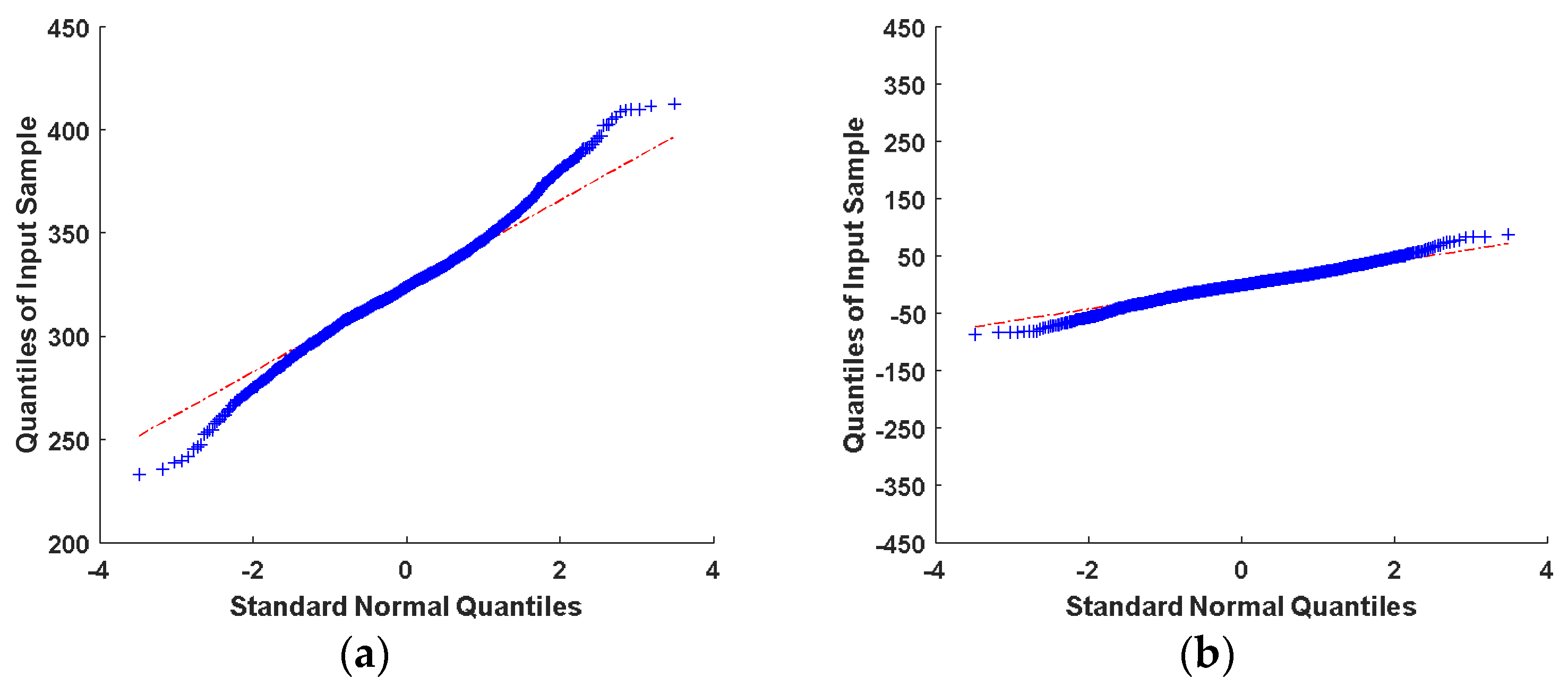
Tm. This is of course far beyond the scope of this study. It is our opinion that trying to derive better empirical-only relations between Tm and Ts, for example by adding a seasonal variation (probably related to the lack of fit at the ends of the QQ plot line in Figure 8), as done by Yao et al. [29] and Bai [35], is going nowhere without a firm understanding of the physics of the atmosphere for high water vapor contents.

Author Contributions

F.Z. conceived and performed the experiments under the supervision of J.-P.B.; F.Z., J.-P.B. and G.X. analyzed the data; F.Z. wrote the paper; and T.-K.Y. provided advice.

Acknowledgments

This research was funded by the French Space Agency (CNES) and the University of French Polynesia. The PhD grant of Fangzhao Zhang is paid for by the French Ministry of Research. We would like to thank the Center for Orbit Determination in Europe (CODE) for providing access to the GPS database, the Integrated Global Radiosonde Archive (IGRA) and Météo-France for providing the radiosonde profiles, and the European Center for Medium-Range Weather Forecasts (ECMWF) for giving access to the gridded VMF1 files (vmf1_g).

Conflicts of Interest

The authors declare no conflict of interest.

References

  1. Parkinson, C.L. Aqua: An Earth-Observing Satellite mission to examine water and other climate variables. IEEE Trans. Geosci. Remote Sens. 2003, 41, 173–183. [Google Scholar] [CrossRef]
  2. Man, S.W.; Jin, X.; Liu, Z.; Nichol, J.E.; Ye, S.; Jiang, P.; Pak, W.C. Geostationary satellite observation of precipitable water vapor using an empirical orthogonal function (eof) based reconstruction technique over eastern china. Remote Sens. 2015, 7, 5879–5900. [Google Scholar] [CrossRef]
  3. Wang, J.; Zhang, L.; Dai, A.; Van Hove, T.; Van Baelen, J. A near-global, 2-hourly data set of atmospheric precipitable water from ground-based GPS measurements. J. Geophys. Res. Atmos. 2007, 112. [Google Scholar] [CrossRef]
  4. Kiehl, J.T.; Trenberth, K.E. Earth’s annual global mean energy budget. Bull. Am. Meteorol. Soc. 1997, 78, 197–208. [Google Scholar] [CrossRef]
  5. Pikridas, C.; Katsougiannopoulos, S.; Zinas, N. A comparative study of zenith tropospheric delay and precipitable water vapor estimates using scientific GPS processing software and web based automated ppp service. Acta Geod. Geophys. 2014, 49, 177–188. [Google Scholar] [CrossRef]
  6. Duan, J.M. GPS meteorology:direct estimation of the absolute value of precipitable water. J. Appl. Meteorol. 1996, 35, 830–838. [Google Scholar] [CrossRef]
  7. King, M.D.; Kaufman, Y.J.; Menzel, W.P.; Tanré, D. Remote sensing of cloud, aerosol, and water vapor properties from the moderate resolution imaging spectrometer (modis). IEEE Trans. Geosci. Remote Sens. 1992, 30, 2–27. [Google Scholar] [CrossRef]
  8. Ross, R.J.; Elliott, W.P. Tropospheric Water Vapor Climatology and Trends over North America: 1973-93. J. Clim. 1996, 9, 3561–3574. [Google Scholar] [CrossRef]
  9. Dessler, A.E.; Zhang, Z.; Yang, P. Water-vapor climate feedback inferred from climate fluctuations, 2003–2008. Geophys. Res. Lett. 2008, 35, 293–310. [Google Scholar] [CrossRef]
  10. Yao, Y.; Shan, L.; Zhao, Q. Establishing a method of short-term rainfall forecasting based on GNSS-derived PWV and its application. Sci. Rep. 2017, 7. [Google Scholar] [CrossRef] [PubMed]
  11. Resch, G.M. Water Vapor Radiometry in Geodetic Applications. In Geodetic Refraction; Springer: Berlin/Heidelberg, Germany, 1984; pp. 53–84. [Google Scholar]
  12. Elliott, W.P.; Gaffen, D.J. On the Utility of Radiosonde Humidity Archives for Climate Studies. Bull. Am. Meteorol. Soc. 1991, 72, 1507–1520. [Google Scholar] [CrossRef]
  13. Ottle, C.; Outalha, S.; Francois, C.; Le Maguer, S. Estimation of total atmospheric water vapor content from split-window radiance measurements. Remote Sens. Environ. 1997, 61, 410–418. [Google Scholar] [CrossRef]
  14. Hanssen, R.F.; Weckwerth, T.M.; Zebker, H.A.; Klees, R. High-Resolution Water Vapor Mapping from Interferometric Radar Measurements. Science 1999, 283, 1297–1299. [Google Scholar] [CrossRef] [PubMed]
  15. Braun, J.; Rocken, C.; Ware, R. Validation of line-of-sight water vapor measurements with GPS. Radio Sci. 2016, 36, 459–472. [Google Scholar] [CrossRef]
  16. Baldysz, Z.; Nykiel, G.; Figurski, M.; Araszkiewicz, A. Assessment of the Impact of GNSS Processing Strategies on the Long-Term Parameters of 20 Years IWV Time Series. Remote Sens. 2018, 10, 496. [Google Scholar] [CrossRef]
  17. Mateus, P.; Nico, G.; Catalão, J. Maps of PWV Temporal Changes by SAR Interferometry: A Study on the Properties of Atmosphere’s Temperature Profiles. IEEE Geosci. Remote Sens. Lett. 2014, 11, 2065–2069. [Google Scholar] [CrossRef]
  18. Mateus, P.; Catalão, J.; Nico, G. Sentinel-1 Interferometric SAR Mapping of Precipitable Water Vapor over a Country-Spanning Area. IEEE Geosci. Remote Sens. Lett. 2017, 55, 2993–2999. [Google Scholar] [CrossRef]
  19. Jiang, P.; Ye, S.; Chen, D.; Liu, Y.; Xia, P. Retrieving Precipitable Water Vapor Data Using GPS Zenith Delays and Global Reanalysis Data in China. Remote Sens. 2016, 8, 389. [Google Scholar] [CrossRef]
  20. Ohtani, R.; Naito, I. Comparisons of GPS-derived precipitable water vapors with radiosonde observations in Japan. J. Geophys. Res. Atmos. 2000, 105, 26917–26929. [Google Scholar] [CrossRef]
  21. Kwon, H.T.; Lim, G.H. Comparison of precipitable water derived from ground-based GPS measurements with NWP analysis over the Korean Peninsula. J. Meteorol. Soc. Jpn. 2008, 85, 733–746. [Google Scholar] [CrossRef]
  22. Choy, S.; Wang, C.S.; Yeh, T.K.; Dawson, J.; Jia, M.; Kuleshov, Y. Precipitable Water Vapor Estimates in the Australian Region from Ground-Based GPS Observations. Adv. Meteorol. 2015, 2015, 1–14. [Google Scholar] [CrossRef]
  23. Janes, H.W.; Langley, R.B.; Newby, S.P. Analysis of tropospheric delay prediction models: Comparisons with ray-tracing and implications for GPS relative positioning. Bull. Géodésique 1991, 65, 151–161. [Google Scholar] [CrossRef]
  24. Flores, A.; Arellano, V.G.D.; Gradinarsky, L.P.; Rius, A. Tomography of the lower troposphere using a small dense network of GPS receivers. IEEE Trans. Geosci. Remote Sens. 2001, 39, 439–447. [Google Scholar] [CrossRef]
  25. Boccolari, M.; Fazlagic, S.; Frontero, P.; Lombroso, L. GPS Zenith Total Delays and Precipitable Water in comparison with special meteorological observations in Verona (Italy) during MAP-SOP. Ann. Geophys. 2002, 45, 599–608. [Google Scholar] [CrossRef]
  26. Alizadeh, M.; Wijaya, D.; Hobiger, T.; Schuh, H.; Weber, R. Atmospheric Effects in Space Geodesy; Springer Atmospheric Sciences; Springer: Berlin, Germany, 2013; pp. 35–71. [Google Scholar]
  27. Davis, J.L.; Herring, T.A.; Shapiro, I.I.; Rogers, A.E.E.; Elgered, G. Geodesy by radio interferometry: Effects of atmospheric modeling errors on estimates of baseline length. Radio Sci. 1985, 20, 1593–1607. [Google Scholar] [CrossRef]
  28. Askne, J.; Nordius, H. Estimation of tropospheric delay for microwaves from surface weather data. Radio Sci. 1987, 22, 379–386. [Google Scholar] [CrossRef]
  29. Yao, Y.B.; Zhu, S.; Yue, S.Q. A globally applicable, season-specific model for estimating the weighted mean temperature of the atmosphere. J. Geodesy 2012, 86, 1125–1135. [Google Scholar] [CrossRef]
  30. Bevis, M.; Businger, S.; Herring, T.A.; Rocken, C.; Anthes, R.A.; Ware, R.H. GPS meteorology: Remote sensing of atmospheric water vapor using the global positioning system. J. Geophys. Res. Atmos. 1992, 97, 15787–15801. [Google Scholar] [CrossRef]
  31. Bevis, M.; Businger, S.; Chiswell, S.; Herring, T.A.; Anthes, R.A.; Rocken, C.; Ware, R.H. GPS Meteorology: Mapping Zenith Wet Delays onto Precipitable Water. J. Appl. Meteorol. 1994, 33, 379–386. [Google Scholar] [CrossRef]
  32. Mendes, V.D.B. Modeling the Neutral-Atmosphere Propagation Delay in Radiometric Space Techniques. Ph.D. Thesis, The University of New Brunswick, Fredericton, NB, Canada, January 1998. [Google Scholar]
  33. Mendes, V.B.; Prates, G.; Santos, L.; Langley, R.B. An Evaluation of the Accuracy of Models for the Determination of the Weighted Mean Temperature of the Atmosphere. In Proceedings of the 2000 National Technical Meeting of the Institute of Navigation, Anaheim, CA, USA, 26–28 January 2000. [Google Scholar]
  34. Liou, Y.A.; Teng, Y.T.; Van Hove, T.; Liljegren, J.C. Comparison of Precipitable Water Observations in the Near Tropics by GPS, Microwave Radiometer, and Radiosondes. J. Appl. Meteorol. Climatol. 2000, 40, 5–15. [Google Scholar] [CrossRef]
  35. Bai, Z. Near-Real-Time GPS Sensing of Atmospheric Water Vapour. Ph.D. Thesis, Tongji University, Shanghai, China, 2005. [Google Scholar]
  36. Wang, J.; Zhang, L.; Dai, A. Global estimates of water-vapor-weighted mean temperature of the atmosphere for GPS applications. J. Geophys. Res. Atmos. 2005, 110. [Google Scholar] [CrossRef]
  37. Raju, C.S.; Saha, K.; Thampi, B.V.; Parameswaran, K. Empirical model for mean temperature for Indian zone and estimation of precipitable water vapor from ground based GPS measurements. Ann. Geophys. 2007, 25, 1935–1948. [Google Scholar] [CrossRef]
  38. Emardson, T.R.; Derks, H.J.P. On the relation between the wet delay and the integrated precipitable water vapour in the European atmosphere. Meteorol. Appl. 2010, 7, 61–68. [Google Scholar] [CrossRef]
  39. Gu, X.; Wang, C.; Wu, D. Research on the local algorithm for weighted atmospheric temperature used in GPS remote sensing water vapor. Sci. Meteorol. Sin. 2005, 25, 79–83. [Google Scholar]
  40. Singh, D.; Ghosh, J.K.; Kashyap, D. Weighted mean temperature model for extra tropical region of India. J. Atmos. Sol. Terr. Phys. 2014, 107, 48–53. [Google Scholar] [CrossRef]
  41. Isioye, O.A.; Combrinck, L.; Botai, J. Modelling weighted mean temperature in the West African region: Implications for GNSS meteorology. Meteorol. Appl. 2016, 23, 614–632. [Google Scholar] [CrossRef]
  42. Zhang, B.; Fan, Q.; Yao, Y.; Xu, C.; Li, X. An Improved Tomography Approach Based on Adaptive Smoothing and Ground Meteorological Observations. Remote Sens. 2017, 9, 886. [Google Scholar] [CrossRef]
  43. Rolf, D.; Simon, L.; Peter, W.; Pierre, F. Bernese GNSS Software Version 5.2; University of Bern, Bern Open Publishing: Bern, Switzerland, 2015; ISBN 978-3-906813-05-9. [Google Scholar]
  44. Pheulpin, L.; Recking, A.; Sichoix, L.; Barriot, J.P. Extreme floods regionalisation in the tropical island of Tahiti, French Polynesia. In Proceedings of the FLOODrisk 2016—3rd European Conference on Flood Risk Management, Lyon, France, 20 October 2016; p. 7. [Google Scholar] [CrossRef]
  45. Serafini, J.; Barriot, J.P.; Sichoix, L. The evolution of precipitable water and precipitation over the Island of Tahiti from hourly to seasonal periods. Int. J. Remote Sens. 2014, 35, 6687–6707. [Google Scholar] [CrossRef]
  46. Zhang, F.Z.; Barriot, J.P.; Keitapu, M.; Sichoix, L. Analysis of the Time Evolution (1974–2017) of Integrated Precipitable Water from Radiosonde Data over French Polynesia. In Proceedings of the 2017 International Conference on Earth Observations and Societal Impacts (ICEO&SI 2017), Yilan, Taiwan, 25–27 June 2017. [Google Scholar]
  47. Haffke, C.; Magnusdottir, G. The South Pacific Convergence Zone in three decades of satellite images. J. Geophys. Res. Atmos. 2013, 118, 10839–10849. [Google Scholar] [CrossRef]
  48. Boehm, J.; Schuh, H. Vienna mapping functions in VLBI analyses. Geophys. Res. Lett. 2004, 31, 195–196. [Google Scholar] [CrossRef]
  49. Steigenberger, P.; Boehm, J.; Tesmer, V. Comparison of GMF/GPT with VMF1/ECMWF and implications for atmospheric loading. J. Geodesy 2009, 83, 943–951. [Google Scholar] [CrossRef]
  50. Boehm, J.; Werl, B.; Schuh, H. Troposphere mapping functions for GPS and very long baseline interferometry from European Centre for Medium-Range Weather Forecasts operational analysis data. J. Geophys. Res. 2006, 111. [Google Scholar] [CrossRef]
  51. Saastamoinen, J. Atmospheric Correction for Troposphere and Stratosphere in Radio Ranging of Satellites. Use Artif. Satell. Geodesy 1972, 247–251. [Google Scholar]
  52. Min, W.; Chai, H.; Pan, Z.; Chen, Y. The Method to Inverse PWV Using VMF1 Grid Data. Lect. Notes Electr. Eng. 2013, 244, 303–310. [Google Scholar]
  53. Durre, I.; Vose, R.S.; Wuertz, D.B. Overview of the Integrated Global Radiosonde Archive. J. Clim. 2006, 19, 53–68. [Google Scholar] [CrossRef]
  54. Durre, I.; Williams, C.N.; Yin, X.; Vose, R.S. Radiosonde-based trends in precipitable water over the Northern Hemisphere: An update. J. Geophys. Res. Atmos. 2009, 114. [Google Scholar] [CrossRef]
  55. Macpherson, B. Radiosonde balloon drift—Does it matter for data assimilation? Meteorol. Appl. 2010, 2, 301–305. [Google Scholar] [CrossRef]
  56. Wiederhold, P.R. Water Vapor Measurement: Methods and Instrumentation; CRC Press: Plymouth, MA, USA, 1997; ISBN 9780824793197. [Google Scholar]
  57. Sun, Y.; Chen, Q.; Gui, K.; Dong, F.; Feng, X.; Long, Q. Characteristics of Water Vapor in the UTLS over the Tibetan Plateau Based on AURA/MLS Observations. Adv. Meteorol. 2017, 2017, 1–13. [Google Scholar] [CrossRef]
  58. Mapes, B.E. Water’s two height scales: The moist adiabat and the radiative troposphere. Q. J. R. Meteorol. Soc. 2001, 127, 2353–2366. [Google Scholar] [CrossRef]
  59. Ross, R.J.; Rosenfeld, S. Estimating mean weighted temperature of the atmosphere for Global Positioning System applications. J. Geophys. Res. Atmos. 1997, 102, 21719–21730. [Google Scholar] [CrossRef]
  60. Kapatou, A. Testing for normality. J. R. Stat. Soc. 1947, 45, 179. [Google Scholar] [CrossRef]
  61. Owens, J.C. Optical refractive index of air: Dependence on pressure, temperature and composition. Appl. Opt. 1967, 6, 51. [Google Scholar] [CrossRef] [PubMed]
  62. Thayer, G.D. An improved equation for the radio refractive index of air. Radio Sci. 2016, 9, 803–807. [Google Scholar] [CrossRef]
  63. Marini, J.W. Correction of Satellite Tracking Data for an Arbitrary Tropospheric Profile. Radio Sci. 1972, 7, 223–231. [Google Scholar] [CrossRef]
  64. Younes, A.M. Evaluation of Wet Mapping Functions Used in Modeling Tropospheric Propagation Delay Effect on GPS Measurements. Open Atmos. Sci. J. 2017, 11, 1–15. [Google Scholar] [CrossRef]
  65. Weaver, C.P.; Ramanathan, V. Deductions from a simple climate model: Factors governing surface temperature and atmospheric thermal structure. J. Geophys. Res. Atmos. 1995, 100, 11585–11591. [Google Scholar] [CrossRef]
Figure 1. The Island of Tahiti, highly dissected by erosion into a net of small radial elongated valleys. The locations of the Geodesy Observatory of Tahiti (International GNSS Service (IGS) Global Positioning System (GPS) receiver ( 149.6064 °   W, 17.5771 °   S), red star) and of the Météo-France weather station (radiosoundings ( 149.6145 °   W, 17.5553 °   S), red circle) are indicated by marks. Figure from Pheulpin et al. [44], with permission.
Remotesensing 10 00758 g001
Figure 2. Left column: Time series from 2011 to 2013 of: (a) estimates of the zenithal total delay (ZTD) from our GPS data processing, our Local VMF1 Processing (LVP) (cyan dots) and Center for Orbit Determination in Europe (CODE) products (magenta dots), and monthly averaged estimates of the ZTD from our GPS data processing (blue dots) and CODE products (red dots), and (c) estimates of the zenith wet delays (ZWD) from our GPS data processing (cyan dots) and CODE products (magenta dots), and monthly averaged estimates of the ZWD from our GPS data processing (blue dots) and CODE products (red dots). Right column: Histogram of (b) the raw ZTD differences between CODE ZTD and LVP ZTD, and (d) the raw ZWD differences between CODE ZWD and LVP ZWD.
Remotesensing 10 00758 g002
Figure 3. Time series from 2014 to 2016 of: (a) estimates of the SAAS_1 ZWD based on Saastamoinen model (LVP ZTD minus SAAS ZHD) (magenta dots) and VMF1 model (cyan dots), and monthly averaged estimates of the SAAS_1 ZWD based on Saastamoinen model (red dots) and VMF1 model (blue dots), and (b) estimates of the SAAS_2 ZWD derived from Saastamoinen model (CODE ZTD minus SAAS ZHD) (magenta dots) and CODE products (cyan dots), and monthly averaged estimates of the SAAS_2 ZWD derived from Saastamoinen model (red dots) and CODE products (blue dots).
Remotesensing 10 00758 g003
Figure 4. (a) Time series from 2014 to 2016 of level 1 radio soundings (RS) precipitable water (PW) from the surface to the 500 hPa level (cyan dots, from the Integrated Global Radiosonde Archive (IGRA) archive) and level 2-A RS PW from the surface to the 500 hPa level (magenta dots), and monthly averaged values of level 1 RS PW from the surface to the 500 hPa level (blue dots) and level 2-A RS PW from the surface to the 500 hPa level (red dots). (b) Relationship between level 2-A PW and level 1 RS PW and their least-squares linear fit (red line).
Remotesensing 10 00758 g004
Figure 5. (a) Time series from 2014 to 2016 of level 2-A RS PW values from the surface to the 500 hPa level (cyan dots) and level 2-B RS PW from the surface to the maximum altitude of the balloon (around 25,500 m, magenta dots), and monthly averaged values of level 2-A RS PW from the surface to the 500 hPa level (blue dots) and level 2-B RS PW from the surface to the maximum altitude of the balloon (red dots). (b) The evolution of the balloon altitude (blue dots) and the PW estimates (red dots) with respect to time at 0:00 on 1 February 2014 (UTC), the green line indicates the altitude of 5500 m (500 hPa), the yellow line indicates the burst of the balloon envelope at 1 h 6 min 52 s after launch and the magenta line indicates the time of the crossing of the 500 hPa level, 15 min 32 s after launch. (c) Relationship between level 2-A PW and level 2-B RS PW and their least-squares fit (red line). This figure is particularly important, as it shows that the difference between the level 2-A and level 2-B is a linear function of the level 2-A values. (d) Relationship between level 1 PW and level 2-B RS PW and their least-squares fit (red line), giving a similar conclusion, as level 1 and level 2-B are consistent (Figure 4b).
Remotesensing 10 00758 g005aRemotesensing 10 00758 g005b
Figure 6. Three-year time series of (a) estimates of our LVP Tm (blue dots), Bevis Tm model (cyan dots) and Tm vmf1_g (red dots), and ((b) partial enlargement of (a)) estimates of Tm from Bevis Tm model (cyan dots) and from vmf1_g (red dots), and monthly averaged estimates of Tm from Bevis Tm model (blue dots) and from vmf1_g (magenta dots).
Remotesensing 10 00758 g006
Figure 7. Relationship between Tm and Ts with (a) LVP raw Tm (blue dots) and the all-seasons least-squares fit (blue line) and the 3-sigma discarded values (red stars), Bevis Tm (magenta dots) based on Bevis Tm model (magenta line), and (b) “Dry” LVP Tm (red dots) based on LVP Tm model in the dry season (from May to October, red line) and “Wet” LVP Tm (green dots) based on LVP Tm model in the wet season (from November to April, green line).
Remotesensing 10 00758 g007
Figure 8. Quantile-Quantile (QQ) plots for (a) raw LVP Tm values (blue dots in Figure 7a); (b) the a posteriori residuals of LVP Tm with regard to the linear fit (line 1 of Table 5). No remaining structure can be found in the residuals of the fits in Figure 8b versus Figure 8a, except maybe at the ends of the QQ line (see the conclusions for a discussion of the origin of this possible misfit).
Remotesensing 10 00758 g008
Figure 9. Time series from 2014 to 2016 of (a) our local mean LVP PW estimates based on all-seasons Tm specific model (blue dots, see Figure 7a) and our mean LVP PW based on season-specific Tm models (red dots, dry or wet depending on the seasons, see Figure 7b), and (b) the differences between the mean PW estimates in Figure 9a. In order to improve legibility, we smoothed the raw PW time series through an averaging window of one month (Equation (14)) to obtain the mean time series shown in Figure 9a.
Remotesensing 10 00758 g009
Figure 10. Time series from 2014 to 2016 of (a) our LVP PW estimates based on our dry season-specific Tm model (cyan dots) and wet season-specific Tm model (blue dots) and level 2-B RS PW estimates from the surface to the maximum altitude of the balloon (red dots). (b) Histogram of the raw PW differences between LVP PW and RS PW of Figure 10a. The monthly averaged time series of the PW values can be found in Figure 12.
Remotesensing 10 00758 g010
Figure 11. Time series from 2014 to 2016 of (a) our LVP PW estimates based on our all-seasons Tm model (blue dots) and level 2-B RS PW estimates from the surface to the maximum altitude of the balloon (red dots). (b) Histogram of the raw PW differences between LVP PW and RS PW. The monthly averaged time series of the PW values can be found in Figure 12.
Remotesensing 10 00758 g011
Figure 12. Time series from 2014 to 2016 of (a) monthly averages of LVP PW based on the all-seasons Tm model (blue dots) and season-specific Tm models (cyan dots) and mean level 2-B RS PW (red dots), and (b) mean PW differences of mean LVP PW based on all seasons Tm model (blue dots) and season-specific Tm models (cyan dots) with RS PW.
Remotesensing 10 00758 g012
Figure 13. Left column: Time series from 2011 to 2014 of: (a) surface pressure recorded by the TAH1 weather station (cyan dots, with some gaps) and surface pressure as downloaded from the vmf1_g (red dots), and monthly averaged surface pressure recorded by the TAH1 weather station (blue dots, with some gaps) and monthly averaged surface pressure as downloaded from the vmf1_g (magenta dots), and (c) surface temperature Ts from the TAH1 weather station (cyan dots, with some gaps) and monthly averaged temperature Ts from the vmf1_g (red dots), and monthly averaged surface temperature Ts from the TAH1 weather station (green dots, with some gaps) and monthly averaged temperature Ts from the vmf1_g (magenta dots). Right column: Time series from 2014 to 2016 of: (b) surface pressure from the vmf1_g (red dots), and monthly averaged surface pressure from the vmf1_g (magenta dots), and (d) surface temperature Ts from the vmf1_g (red dots), and monthly averaged surface temperature Ts from the vmf1_g (magenta dots).
Remotesensing 10 00758 g013
Table 1. Statistical summary for the comparison between our LVP ZTD and ZWD and CODE products (LVP minus CODE) in terms of max, min, bias, STD, and RMS, from 2011 to 2013, relative to Figure 2b,d.
Data DifferencesMax (mm)Min (mm)Bias (mm)STD (mm)RMS (mm)Data Points
ZTD19.91−19.80−0.246.106.1112,702
ZWD20.17−19.64−0.166.116.1212,702
Table 2. Statistical summary for the comparisons between our LVP ZWD estimates and SAAS_1 ZWD estimates (LVP minus SAAS_1), CODE ZWD and SAAS_2 ZWD estimates (CODE minus SAAS_2) in terms of max, min, bias, STD and RMS, from 2014 to 2016, relative to Figure 3a,b.
Data DifferencesMax (mm)Min (mm)Bias (mm)STD (mm)RMS (mm)Data Points
LVP-SAAS_14.95−10.000.851.211.484178
CODE-SAAS_24.72−3.570.691.161.354178
Table 3. Statistical summary for the comparison between level 1 RS PW estimates and level 2-A RS PW estimates (level 1 minus level 2-A) in terms of max, min, bias, STD, and RMS, from 2014 to 2016.
PW DifferencesMax (mm)Min (mm)Bias (mm)STD (mm)RMS (mm)Data Points
Level 1-2-A6.21−5.22−0.101.301.302151
Table 4. Summary for the comparison between the level 2-A RS PW estimates from the surface to the 500 hPa level and level 2-B RS PW estimates from the surface to the maximum altitude of the balloon (the latter minus the former) in terms of max, min, bias, STD and RMS, from 2014 to 2016, relative to Figure 5b.
PW DifferencesMax (mm)Min (mm)Bias (mm)STD (mm)RMS (mm)Data Points
Level 214.19−19.242.752.323.602179
Table 5. Intercept and slope of our new on-site Tm models for all-seasons and the two different tropical seasons (dry and wet). Number of data points fitted: 2060, number of data points deleted by applying the 3-sigma rule: 33.
Tm ModelInterceptSigmaSlopeSigma
All seasons−476.44145.552.680.49
Dry season−535.69252.912.890.85
Wet season−979.71226.864.360.76
Table 6. Statistical summary of the comparison between our LVP PW estimates based on our season-specific Tm models and level 2-B RS PW (LVP PW minus RS PW) in terms of max, min, bias, STD and RMS, from 2014 to 2016, relative to Figure 10b.
PW DifferencesMax (mm)Min (mm)Bias (mm)STD (mm)RMS (mm)Data Points
LVP-level 2-B RS19.29−14.910.143.293.292060
Table 7. Statistical summary for the comparison between our LVP PW estimates based on our all-seasons Tm model and level 2 RS PW values (LVP minus RS) in terms of max, min, bias, STD, and RMS, from 2014 to 2016, relative to Figure 11b.
PW DifferencesMax (mm)Min (mm)Bias (mm)STD (mm)RMS (mm)Data Points
LVP-RS53.87−27.500.044.294.292060
Table 8. Statistical summary for the comparison between monthly averaged surface pressure and temperatures Ts from the gridded VMF1 files and from TAH1 weather station (vmf1_g minus TAH1) in terms of max, min, bias, STD, and RMS, from 2011 to 2014, relative to Figure 13a,c.
Mean DifferencesMaxMinBiasSTDRMSData Points
Pressure (hPa)−0.21−1.20−0.460.140.484882
Ts (K)0.15−1.51−0.730.360.814882

