Single Channel Circular SAR Moving Target Detection Based on Logarithm Background Subtraction Algorithm

Abstract

In this paper, a new moving target detection algorithm for single channel circular Synthetic Aperture Radar (SAR) is presented. Circular SAR can perform observation with circular trajectory and retrieve multiaspect information. Due to the circular trajectory, the moving target has long and complex apparent trace (smear trajectory), while the background (clutter) has relatively slow changing characteristic in limited azimuth integration. Thus, the background image can be filtered by using radiometric adjusted overlap subaperture images. Then, the Signal-to-Clutter Ratio (SCR) of the region where the strong backscattering clutter exists is enhanced with logarithm background subtraction technique. In the real data experiment, the maximum SCR improvement is 13 dB. Finally, the moving target can be detected using a Constant False Alarm (CFAR) detector. The algorithm is evaluated with one channel data of three channel GOTCHA-GMTI dataset.

1. Introduction

Due to its high resolution imaging and all weather capabilities, synthetic aperture radar (SAR) has become an important technique in remote sensing area. Ground moving target detection with SAR sensor is one of the challenging tasks in applications such as battle field surveillance and city traffic monitoring [1,2].

Thus far, detecting moving targets with SAR sensor mainly by performing clutter cancellation which is achieved with multichannel techniques such as Displaced Phase Center Array (DPCA) [3], Along-Track Interferometry (ATI) [4] and Space-Time Adaptive Processing (STAP) [5,6]. Such techniques have now been implemented on multiple airborne/spaceborne multichannel SAR systems such as PAMIR [2], and RADARSAT-2 [7]. The performance of detection can be improved by increasing the number of channels. However, with the number of channels increased, such system usually has high cost and high system complexity. Single channel methods play another important role in moving target detection application. Single channel moving target detection methods utilize the delocalization (Doppler shift) and defocusing characteristics of the moving target signature in SAR image. Methods utilizing Doppler shift cannot detect targets whose spectrum within the clutter spectrum [8]. Method utilizing defocusing characteristic usually have heavy computational burden due to the iteration process [9,10]. The above disadvantages limit the application of single channel system. However, with recent research development in Circular SAR, the single channel system can fulfill the requirement of moving target detection task.

Circular SAR is a new SAR acquisition mode first introduced in 1996 [11]. The SAR sensor performs circular flight while the main beam points to the scene of interest during the observation. This new imaging mode is validated with airborne experiments by several institutes [12,13,14,15]. The circular track causes difficulties in SAR signal processing. Thus, current CSAR studies are focusing on stationary scene/target application such as high resolution imaging [16], DEM estimation [17], concealed targets detection [18], etc. Comparing with CSAR stationary scene studies, the studies on CSAR moving target issue are just beginning.

In early research, researchers use long time observation characteristic of circular SAR to obtain the echo of moving target in the illuminated scene [19,20,21]. Many researchers have realized potential of using image sequence to detect moving targets in single channel SAR such as [20,22,23]. In 2015, Poisson et al. [24] proposed a single channel algorithm to reconstruct the real trajectory and estimate the velocity which focuses on using circular SAR properties . The algorithm uses target apparent position along circular flight to calculate the real position and velocity. However, the moving target detection method is not discussed. Thus, this paper focuses on proposing a moving target detection algorithm for single channel circular SAR.

Circular SAR is sensitive to slow moving targets due to long time observation. Because of circular track, radar can get the information of target’s radial velocity from multiple azimuth viewing angles which is good for velocity estimation. A moving target tends to be delocalized because of range speed and defocused because of azimuth speed and range acceleration [8]. On the one hand, the target’s signature shifts to the different position on SAR subaperture image due to the radar’s circular track. On the other hand, static scene has several angular sectors where its scattered fields are varying slowly [25]. Therefore, the background image can be filtered due to pixel value of static scene change severely when the target’s signature moves onto and leaves it. Then, targets can be detected by comparing the original subaperture images and background image. Moreover, the log-ratio operator is integrated into the proposed algorithm to achieve good clutter suppression result. The proposed algorithm includes the following steps. First, the Back Project (BP) algorithm is used to generate overlap subaperture logarithm images. Then, radiometric adjustment is applied to remove the antenna illumination effect. Next, the median filter is applied to the image sequence to get the background image. Finally, after subtracting the background to enhance the signal-to-clutter-ratio, the moving targets can be detected with CFAR algorithm.

The rest of the paper is organized as follows. In Section 2, we analyze the moving target signal model because of the complex radar target relative motion. The moving target apparent position calculation equations are also introduced and demonstrated with point target simulation. Using these equations, we locate the moving target in SAR image. Then, a brief comparison of the target’s apparent trace under linear and circular flight for proposed detection algorithm is presented. In Section 3, we give a detailed description of logarithm background subtraction algorithm. 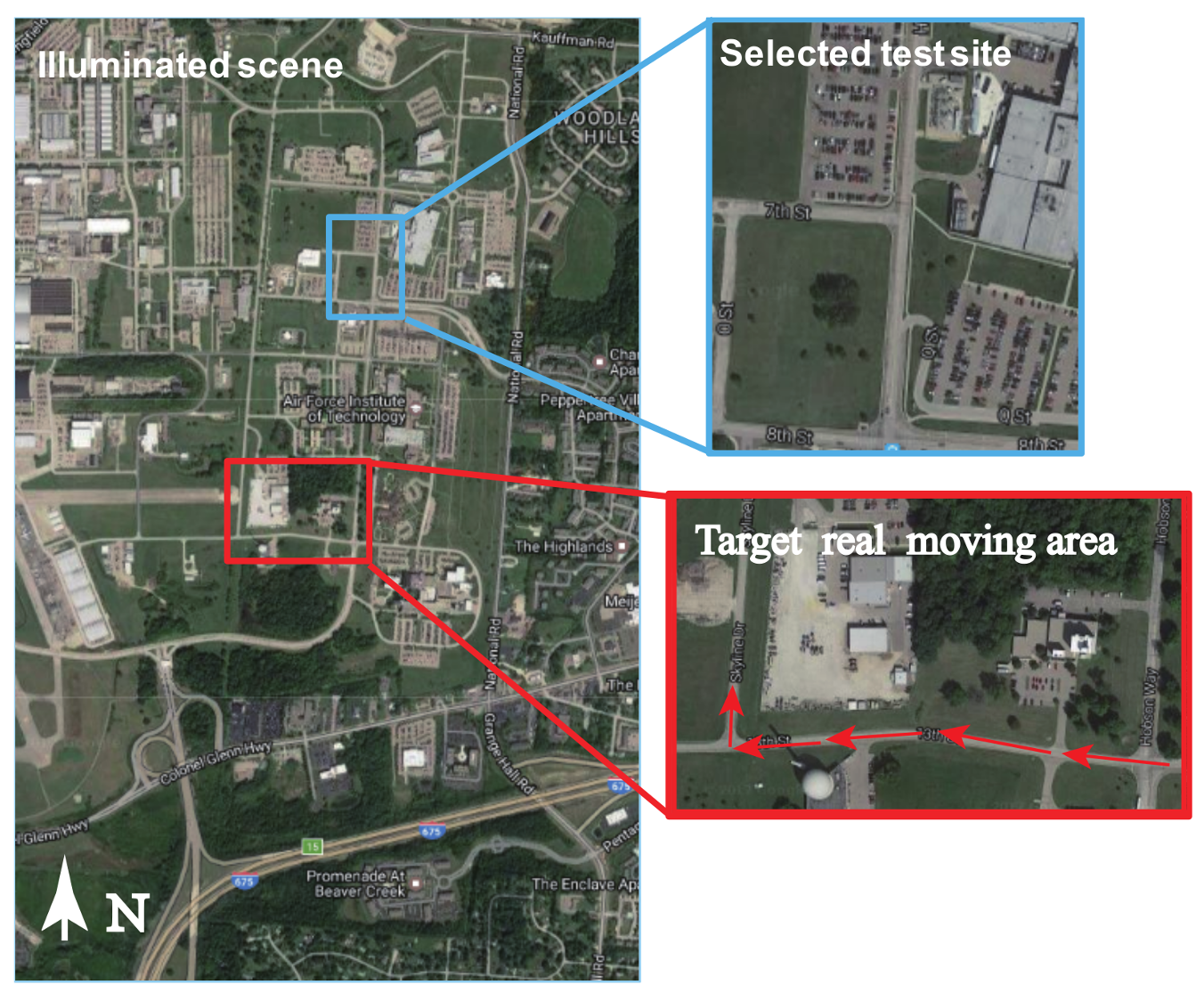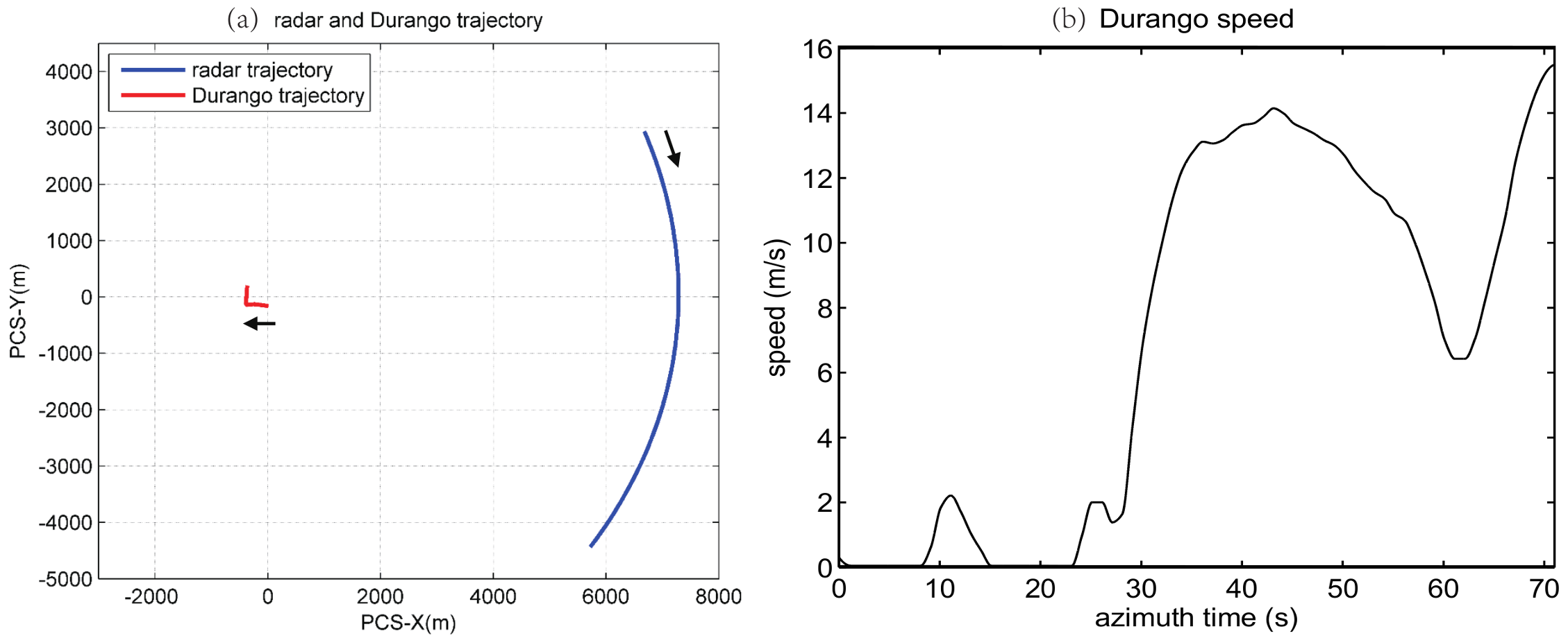In Section 4, we use one channel data of three channel airborne GOTCHA-GMTI dataset [26] to validate proposed logarithm background subtraction algorithm. Section 5 is the conclusion.

2. Moving Target Signal Model

In this section, the moving target signal model is presented. Apparent position calculation equations for arbitrary motion are described based on equal range equal Doppler principle. Then, the point target simulation and a brief comparison of target’s apparent trace morphology under circular and linear flight case are presented.

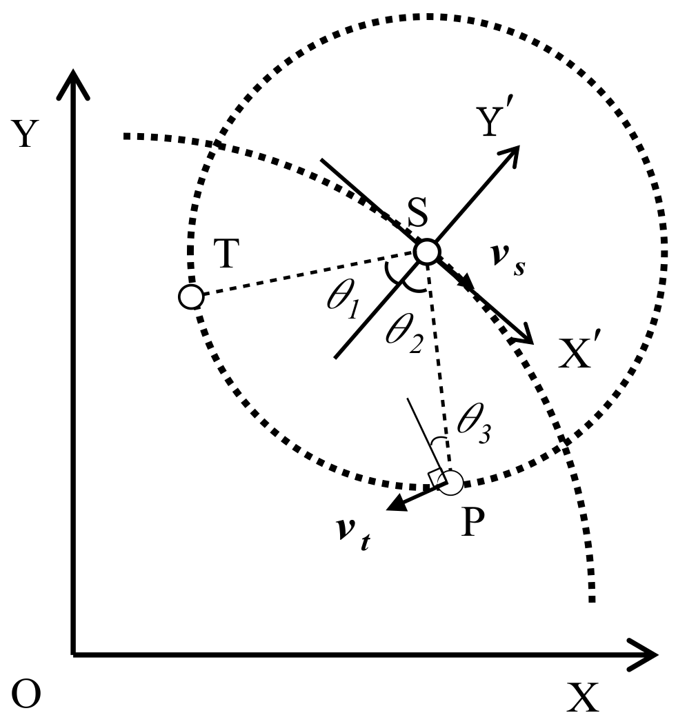
For mathematical convenience, here we assume the moving target is an isotropic point target during the observation. The top view of the coordinate system is shown in Figure 1. $XOY$ is the ground coordinate system. The radar performs a circular flight path at height $H_0$ with constant speed $v_S$. During the illumination, the main beam points to the scene center O. Here, we assume target’s motion is confined in ground plane and is illuminated by radar main beam. At time $t_0$, Radar position is denoted by S, target real position is denoted by P. $v_t$ is target’s instantaneous speed. $X^{\prime }S{Y}^{\prime }$ represents the radar coordinate system. After SAR processing, target appears at position T in SAR image because of target motion.

To calculate target’s apparent position in SAR image, we can use equal range equal Doppler equations. Because the two-way transmission time is fixed, distance of target to the radar and distance of target’s apparent position to radar are equal. Thus, the equal range relation is given by

$$|\overrightarrow{SP}|=|\overrightarrow{ST}|$$

(1)

Due to the number of unknowns, we need an extra equation to get the target image position. This can be fulfilled with equal Doppler equation. Doppler term of moving target has two parts: (1) radar motion induced part; and (2) target motion induced part. Thus, the Doppler frequency of moving target $f_P$ is

$$f_P=\frac{2·v_s·\sin {\theta }_2}{\lambda }-\frac{2·v_t·\sin {\theta }_3}{\lambda }$$

(2)

When forming the SAR image, target will appear at T. The corresponding Doppler frequency $f_T$ is given by

$$f_T=\frac{2·v_s·\sin {\theta }_1}{\lambda }$$

(3)

Combining Equations (2) and (3), we can get the equal Doppler equation.

$$v_s·\sin {\theta }_1=v_s·\sin {\theta }_2-v_t·\sin {\theta }_3$$

(4)

For consideration of generality, we rewrite Equation (4) into vector form below.

$$\overrightarrow{v_s}·\overrightarrow{ST}=\overrightarrow{v_s}·\overrightarrow{SP}-\overrightarrow{v_t}·\overrightarrow{SP}$$

(5)

From mathematical point of view, Equation (5) sets a line across T and S. Thus, there are two solutions. The false solution can be excluded by constrain of beam pointing direction. Finally, the system to calculate the target’s apparent position is obtained:

$$\left\{\begin{array}{ccc}\hfill \overrightarrow{v_s}·\overrightarrow{ST}& =& \overrightarrow{v_s}·\overrightarrow{SP}-\overrightarrow{v_t}·\overrightarrow{SP}\hfill \\ \hfill |\overrightarrow{SP}|& =& |\overrightarrow{ST}|\hfill \\ \hfill |\overrightarrow{OP}|& <& |\overrightarrow{OS}|\hfill \end{array}\right.$$

(6)

Using the vector form, the moving target apparent trace in imaging plane can be computed even when the radar trajectory deviates from standard circular flight. In the above deduction, target motion induced Doppler ambiguity problem is not taken into consideration.

From Equation (6), under side-looking imaging condition, there are two special cases. If target velocity coincides with line-of-sight (LOS), which means target only has range speed at that moment. Then, the target’s apparent position has maximum shift in azimuth. If target velocity is perpendicular to LOS (only azimuth speed), then the target apparent trace shall appear at its true location.

In system Equation (6), the instantaneous target apparent position only relates to the target’s velocity and radar position and velocity at that time. Thus, Equation (6) are not confined by radar observation geometry or target motion form. From this point of view, the defocusing effect has another interpretation. Target apparent position has a slight difference due to target Doppler changes at each azimuth sample time within azimuth integration, thus causing the defocusing.

To further demonstrate the effectiveness of Equation (6), the simulation experiment is shown.

Table 1. SAR parameters.

Symbol	SAR Parameters	Value
$f_c$	Center frequency	9.6 GHz
$B_d$	Bandwidth	640 MHz
$prf$	Pulse repetition frequency	1.32 kHz
$r_c$	Range to scene center	3000 m
${\theta }_{inc}$	Incidence angle	${45}^{\circ }$
$v_s$	Radar speed	200 m/s
${\theta }_{azi}$	Azimuth integration angle	${180}^{\circ }({90}^{\circ }\sim -{90}^{\circ })$

is the SAR parameters for simulation. Radar flight is half circle and flying direction is clockwise from ${90}^{\circ }\sim -{90}^{\circ }$. The radar works in side-looking mode is assumed.

The target motion uses the simplest form in simulation, i.e., moving with constant speed. Traditional analysis about moving targets are mainly focused on two cases: target has range speed and target has azimuth speed. In circular SAR mode, the azimuth viewing angle changes along time, and target can be seen in 360 degrees. However, when considering the half circle case, a similar analysis can be performed. Two targets with different moving direction are simulated, respectively. One moves along X-axis from positive to negative. The other one has similar configuration, but along Y-axis. Moving targets motion parameters are shown in

Table 2. Targets parameters.

Parameters	Target 1	Target 2
speed	−4 m/s	4 m/s
moving direction	180°	90°
start point	(94.2, 0) m	(0, −94.2) m

.

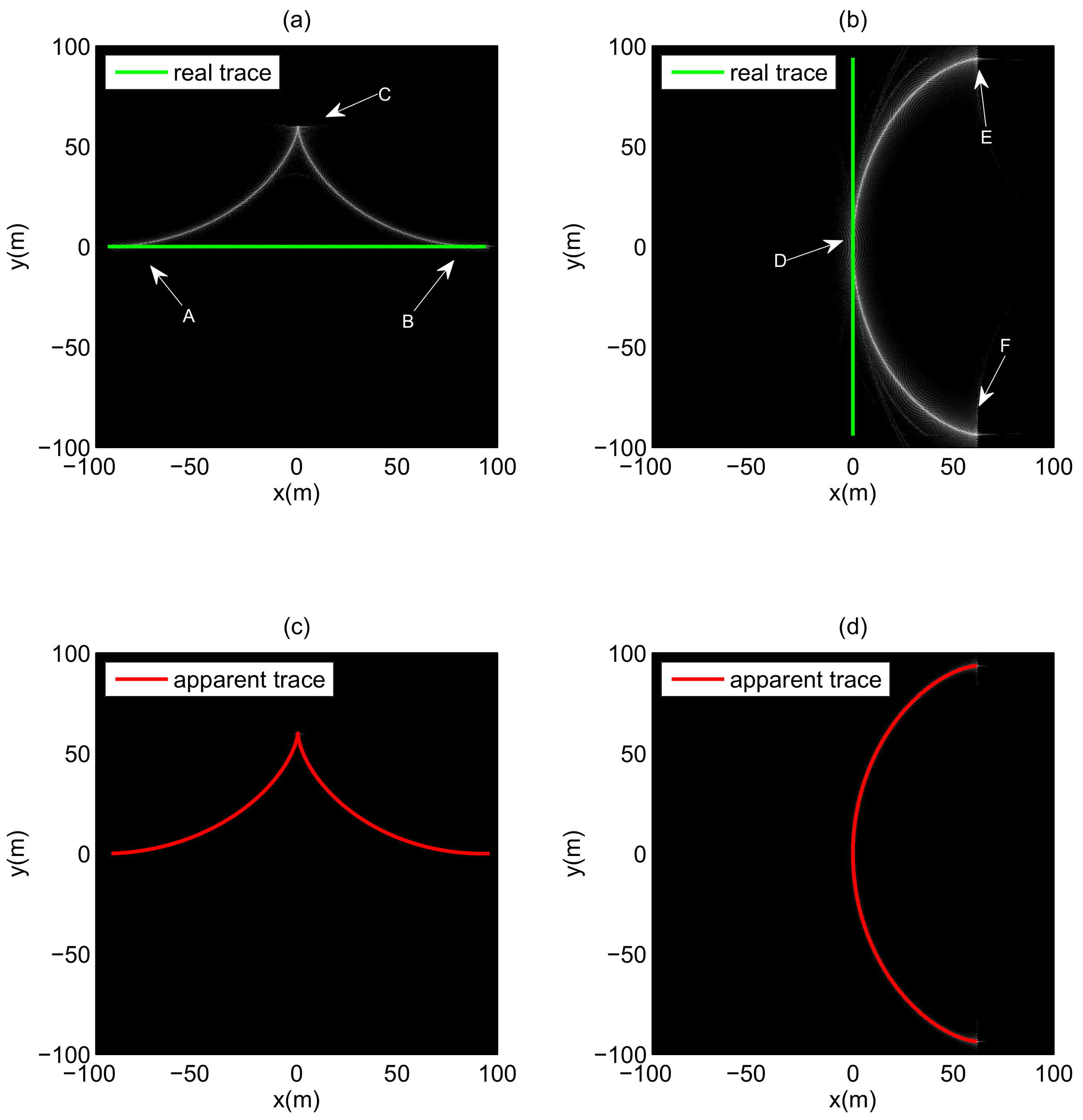
The simulation result is shown in Figure 2. Left and right columns are Target 1 and Target 2 experiment results, respectively. First row is their SAR images. All azimuth data are coherently integrated. It is clear that the target apparent trace pattern is more complex than in linear SAR mode whose observation geometry is a straight line. It is not the elliptic or hyperbolic shape mentioned in [27,28].

The green line denotes target real trace. In Figure 2a, the target smear signature coincides with target real trace at A and B. This is because the target velocity is perpendicular to LOS at that moment, as analysis presented in Section 2. The maximum shift position is C. Target velocity coincides with LOS at that moment. Figure 2b has the same special cases as D, E, and F. Second Row is the SAR image superimposed with apparent trace calculated by system Equation (6). It is obvious that the calculated apparent trace matches the smear signature in SAR image. The effectiveness of system Equation (6) is therefore validated.

As mentioned in Section 2, Equation (6) is not confined by circular flight. We use Equation (6) to make a comparison between the circular and linear radar flight to further demonstrate the characteristic of target apparent trace under circular flight.

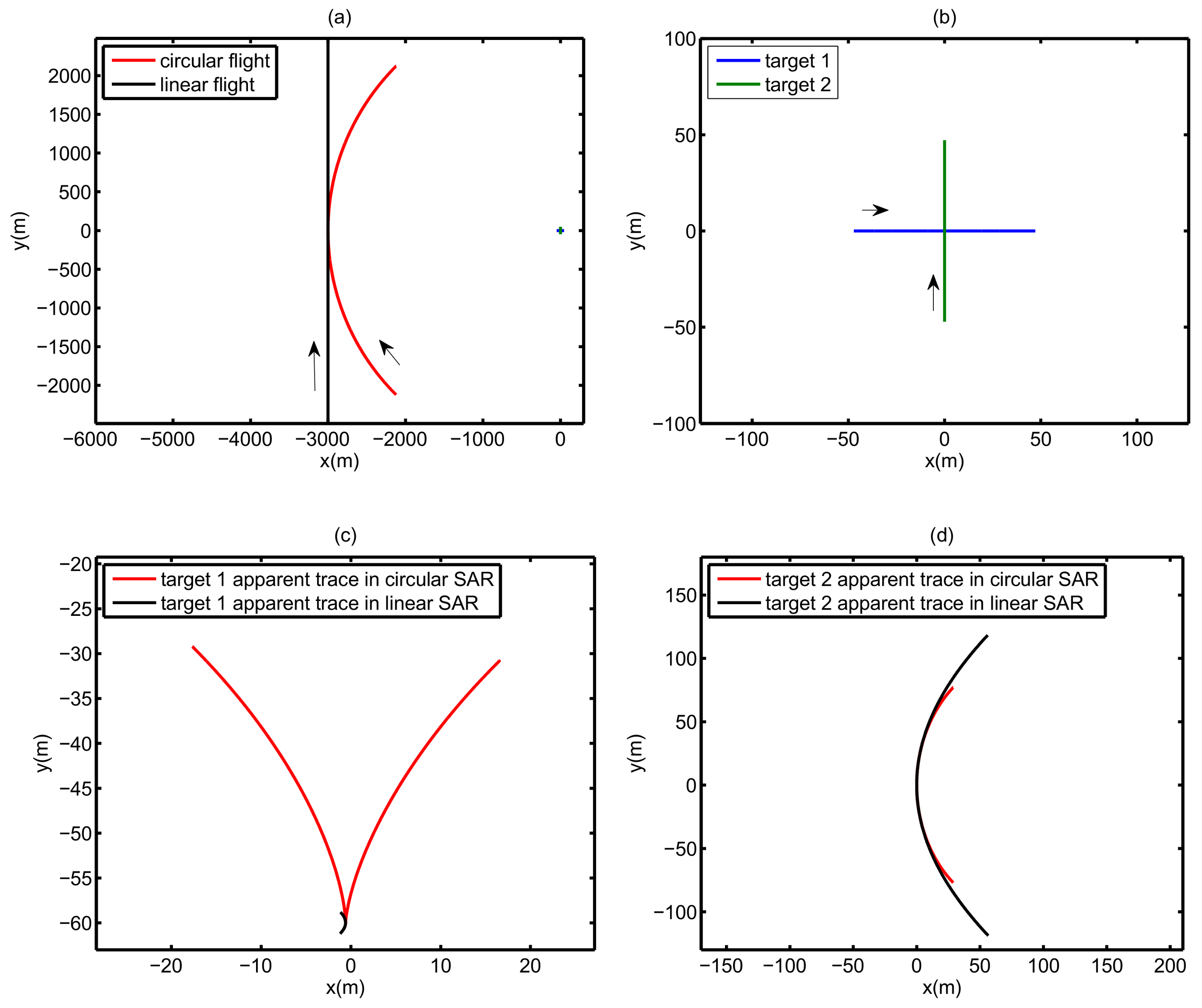
Figure 3 is the comparison of moving target apparent trace in circular SAR and in linear SAR. Red line denotes the circular SAR results, and linear SAR results are denoted with black line. Figure 3a is the top view of target radar geometry. The radar speed is 200 m/s, and both azimuth integration angles are ${90}^{\circ }$. For convenience, the radar and the targets are moving at height 0 m. Two types of moving targets are simulated in circular SAR mode and linear SAR mode, respectively, as shown in Figure 3a in the right small area and enlarged in the picture in Figure 3b. Target 1 moves along X-axis (only has range speed), while Target 2 moves along Y-axis (only has azimuth speed). Their speed is 4 m/s. Figure 3c is apparent trace of Target 1 in circular SAR and linear SAR, and their lengths along X-axis are 34.24 m and 0.62 m, and along Y-axis are 30.79 m and 2.39 m, respectively. The apparent trace of Target 1 in circular SAR spans more areas than in linear SAR. The apparent trace in linear SAR only occupies several resolution cells even under ${90}^{\circ }$ synthetic aperture which makes it hard to differentiate from the stationary target (in SAR image domain). In Figure 3d, in circular SAR, the lengths of apparent trace along X-axis and Y-axis are 28.8 m and 153.9 m, respectively. In linear SAR, the lengths are 56.5 m and 237.1 m, respectively. The apparent trace of Target 2 spans over 100 m at azimuth direction in both cases.

Most detecting moving targets in image domain algorithms take advantage of target image motion in subaperture images, which means it requires long apparent trace. Thus, theoretically, in linear SAR, only target with azimuth speed has high chance to be detected and difficult for those only with range speed. Hence, for wide aperture case, the circular flight is better than linear flight in moving target detection using subaperture image sequence.

3. Logarithm Background Subtraction

In this part, we give details about the logarithm background subtraction.

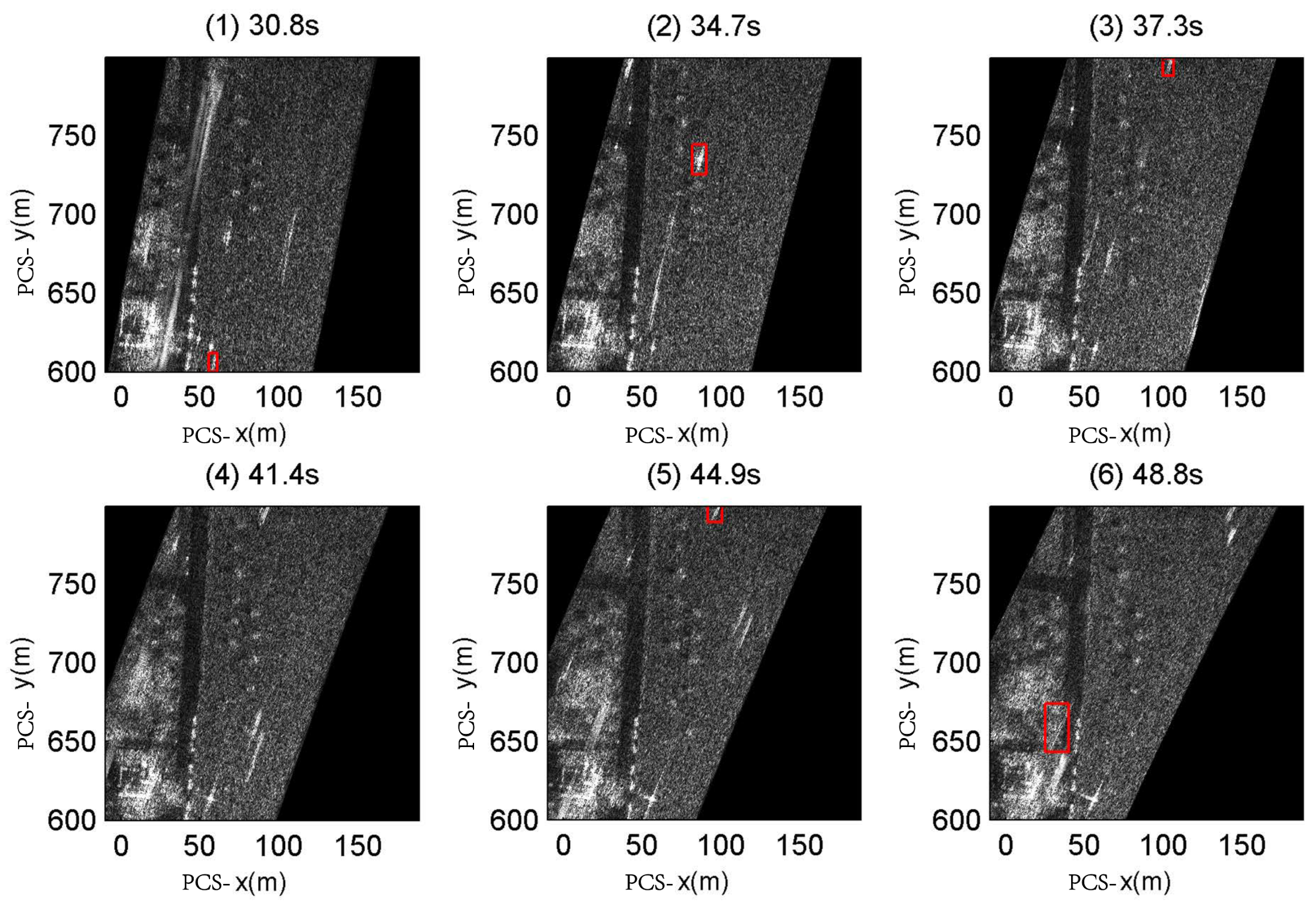
A subaperture image can be seen as combination of background image (contain clutter) and foreground image (contain moving target). For clutter, its scattered field is varying slowly in limit angular sector. For moving target, its image position is changing along azimuth viewing angle because of circular flight. Hence, the target has complex apparent trace form than linear SAR mode whose radar observation geometry is a straight line. From subaperture point of view, target signature is moving in consecutive subaperture images. Thus, value of certain pixel would have sudden change when target signature is moving onto and leaving it. According to analysis, the median filter is selected to generating background image (clutter). The SCR is improved after subtraction processing. The log-ratio operator is integrated into the process. The operator can be defined as the logarithm of the ratio of two images. This is equal to the subtraction of two logarithm images. Finally, the moving target can be detected by applying CFAR detector.

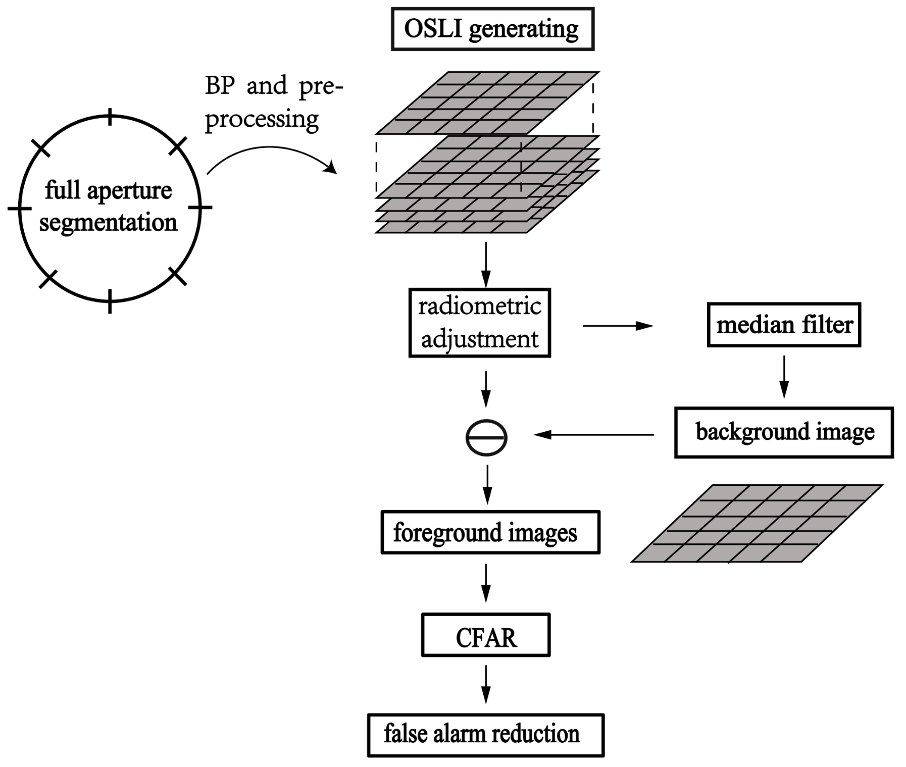
The processing chain is shown in Figure 4. The processing chain of the algorithm has following parts: (1) segment the full aperture into N arcs with equal length; (2) for each arc, using the same image grid to generate M overlap subaperture images (in dB unit) , perform preprocessing to form the Overlap Subaperture Logarithm Image (OSLI) sequence; (3) perform radiometric adjustment process on each OSLI sequence; (4) apply median filter along the azimuth time dimension to the OSLI sequence to get corresponding background image; (5) generate foreground images by using OSLI subtracts the background image; and (6) target detected on foreground images with the CFAR algorithm.

In the following, the details are presented.

3.1. Preprocessing and OSLI Generating

The segmentation issue is related to the anisotropic backscatter behavior and target motion. If azimuth angle of each arc is too wide, then scattered field of static scene might change too much. Therefore, the background image cannot be well modeled. On the other hand, if the angle is too narrow, then the target defocusing signature may not exceed certain pixels in image sequence. Thus, there might be residual target signature remain in filtered background image. This will deteriorate the detection performance. Thus far, this aperture partition parameter is set by experimental test, while the optimal partition criterion is still being researched.

After, the full aperture is divided into N arcs using the echo of ith arc to generating M overlap subaperture intensity images $\{I(j)|j=1\dots M\}$. The reason for forming overlap images is that they can provides more azimuth sampling data for each pixel. The overlap images are good for target tracking due to the target image motion continuity is preserved. The algorithm to form the SAR image is the time domain back projection algorithm (BP). BP is a typical SAR imaging algorithm which can handle the circular radar observation geometry. There are several kinds of fast algorithms to reduce computational burden [16,29] in practical application. The most important component is that the images can be formed with the same image grid, thus avoiding applying an extra image coregister step. Other imaging algorithms can also be applied, such as polar format algorithm [30]. However, the image coregister step should be applied and the error due to the mismatch should be taken into consideration.

The next step is suppressing the speckle noise. For jth intensity image $I(j)$, a $5\times 5$ averaging cell to despeckle noise is used. Finally, the OSLI sequence is obtained by transforming the images into dB units and indexing with azimuth time. The overall expression in this subsection is given by Equation (7)

$$\begin{array}{c}\hfill \begin{array}{c}\hfill OSL{I}_i={\displaystyle \bigcup _{j=1}^M}\log [I(j)],i=1,2,\dots ,N.\end{array}\end{array}$$

(7)

3.2. Radiometric Adjustment

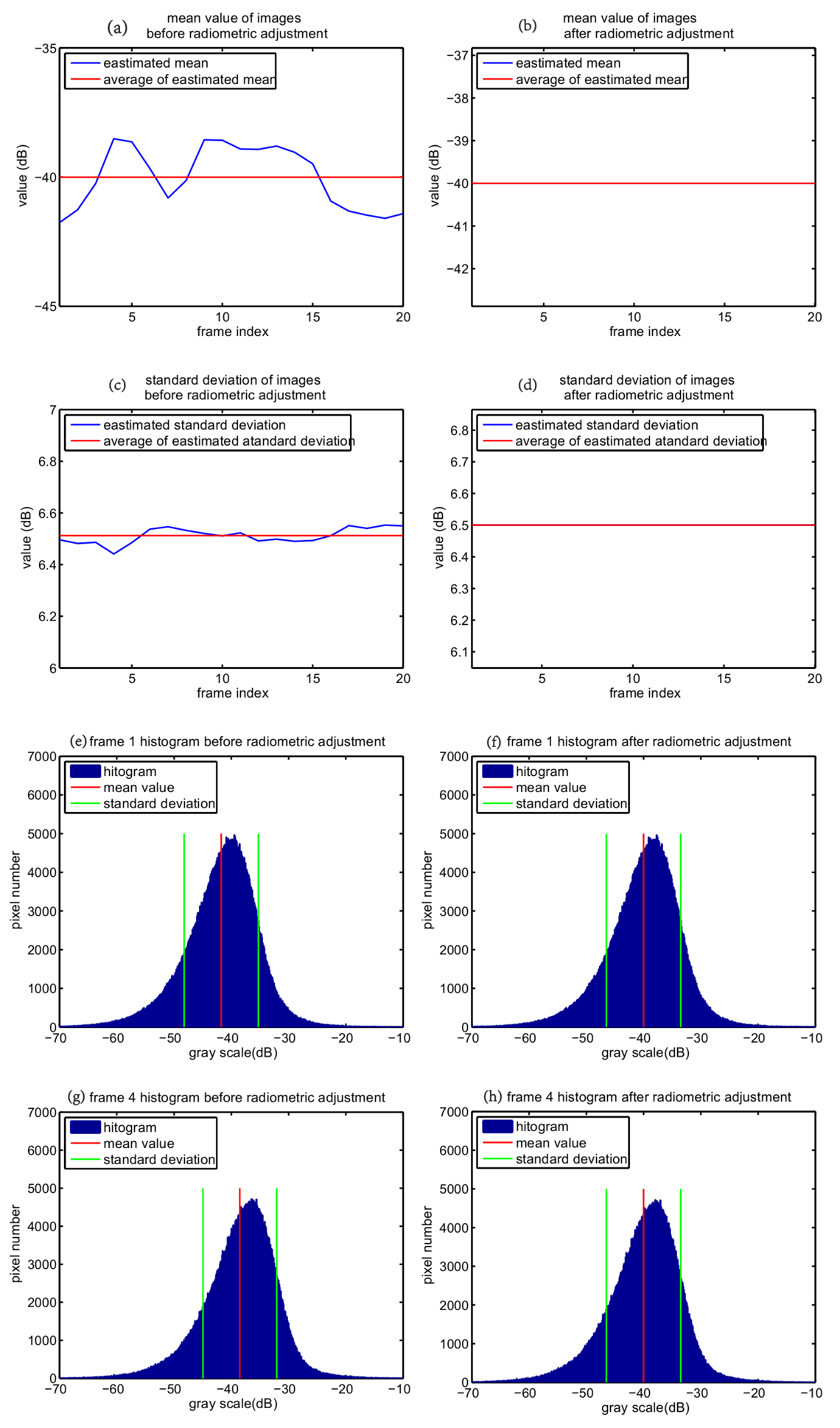
One of the basic assumptions of this algorithm is that the pixel value of the static clutter is only changing along azimuth viewing angle. In practice, however, it is influenced by antenna pattern anisotropy [25]. If the illumination variation between images cannot be well compensated, there will be false alarms. The circular path makes this problem more difficult. Thus, a simple method called Intensity Normalization is adopted.

This method can adjust the pixel values in each image have the same mean value and standard deviation [31]. In our algorithm, we first collect the mean value and standard deviation from each image in ith OSLI as in Equation (8).

$$\begin{array}{cc}\hfill {\mu }_j& =E[log[I(j)]]\hfill \\ \hfill {\sigma }_j& =\sqrt{E{\{[log[I(j)]-{\mu }_j]}^2\}}\hfill \end{array}$$

(8)

${\mu }_j$ and ${\sigma }_j$ are mean value and standard deviation of jth image. Then, calculate the average of collected data as the new mean value and standard deviation.

$$\begin{array}{cc}\hfill {\mu }_0& =\frac{1}{M}{\displaystyle \sum _{j=1}^M}{\mu }_j\hfill \\ \hfill {\sigma }_0& =\frac{1}{M}{\displaystyle \sum _{j=1}^M}{\sigma }_j\hfill \end{array}$$

(9)

Apply intensity normalization method to each image with ${\mu }_0$ and ${\sigma }_0$, as shown in Equation (10).

$$\widetilde{\log [I(j)]}=\frac{{\sigma }_j}{{\sigma }_0}(\log [I(j)]-{\mu }_j)+{\mu }_0$$

(10)

The $\widetilde{\log [I(j)]}$ is the new images which can be seen as without illumination variation and as input data for background generating.

3.3. Background Generating and Subtraction

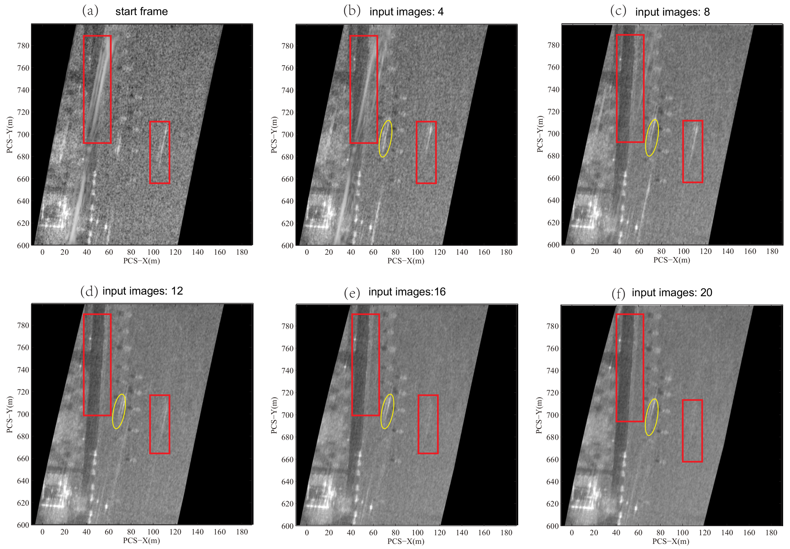
Filtering out the background image is a key step in this algorithm. As the analysis presented in above section, the target signature will cause pixel with sudden change (high value) when it moves onto the pixel. The median filter is selected to model the background images because it can exclude the high value in a series of numbers. Taking a pixel in OSLI as an example, the median filter sorts the input values of certain pixel from all input subaperture images and then pick the middle element from the sorted data as the pixel value in the background image. The background image $\log [B_i]$ corresponding to ith radiometric adjusted $\widetilde{OSL{I}_i}$ is obtained by

$$\begin{array}{cc}\hfill \log [B_i]& =median\{\widetilde{OSL{I}_i}\}\hfill \\ & =median\{{\displaystyle \bigcup _{j=1}^M}\widetilde{\log [I(j)]}\}\hfill \end{array}$$

(11)

The output background image is expressed in dB unit. For mathematical convenience, we use $\log [B_i]$ to denote it. ${\displaystyle \bigcup _{j=1}^M}\widetilde{\log [I(j)]}$ is the ith OSLI sequence which has performed the intensity normalization.

Next, the foreground image sequence is obtained by using the input images to subtract the background image, which is given by Equation (12):

$$\log [F(j)]=\widetilde{\log [I(j)]}-\log [B_i],j=1,2,\dots ,M.$$

(12)

$\log [F(j)]$ denotes the jth output image in the foreground image sequence.

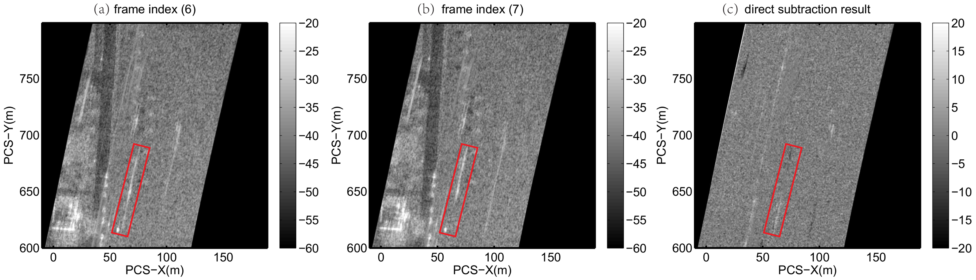
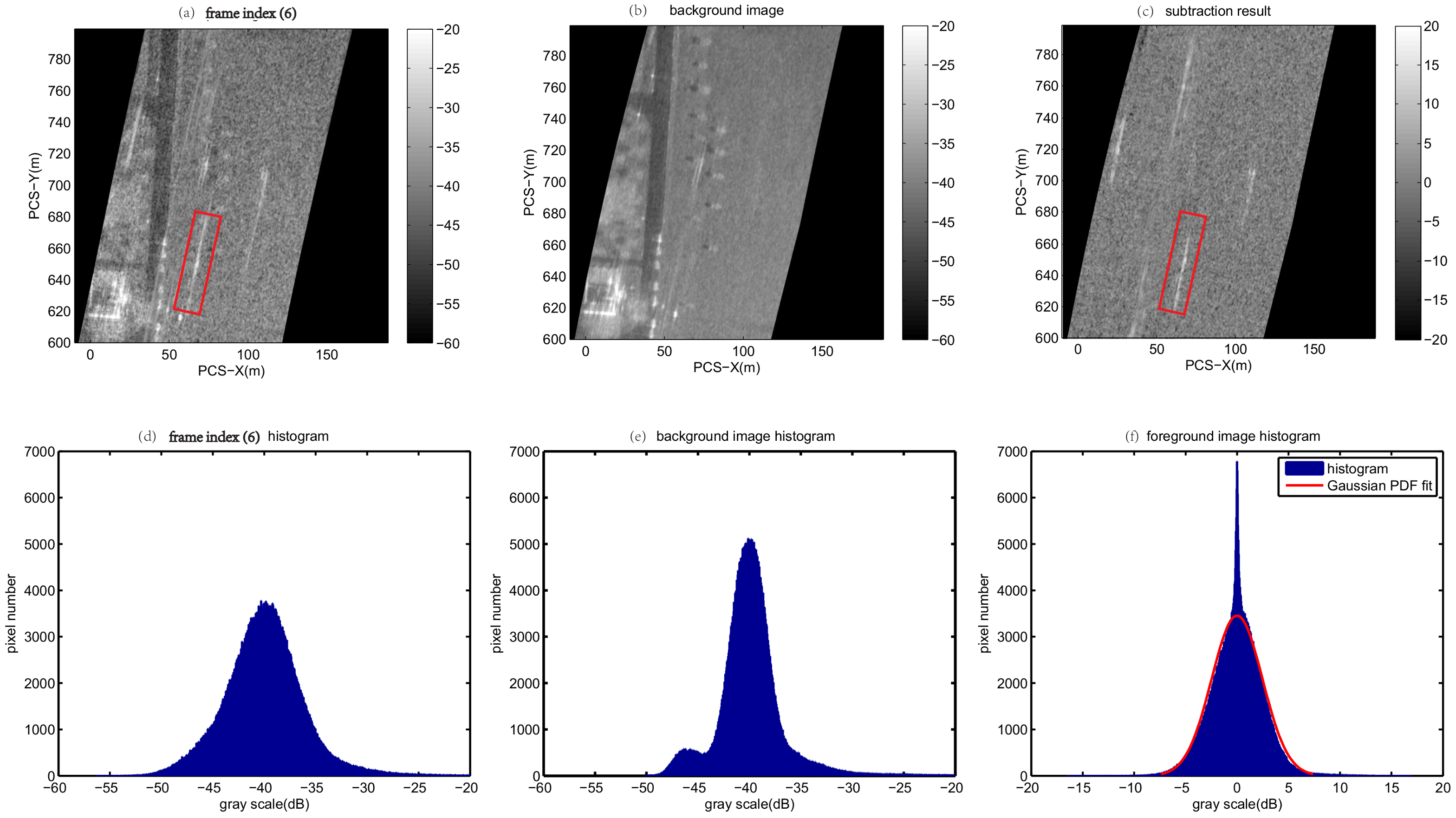
In Equation (12), the right two terms are in logarithm form. Thus, it can also be interpreted as image-ratio in logarithm form, i.e the famous log-ratio operator [32,33]. Due to the image-ratio process, the canceled clutter part lies near the zero in the foreground image histogram. The moving target part will fall into the foreground image histogram tail. The Gaussian distribution has been used on the image processed by log-ratio operator, as demonstrated in [32]. The Gaussian distribution fits the histogram of foreground image, as shown in the real data experiment.

3.4. CFAR Detection

In this section, two parameter CFAR detector [34] to detect the moving targets in the foreground images. As mentioned above, the Gaussian distribution is assumed. The Gaussian distribution characterizing the foreground image statistic is given by

$$p=\frac{1}{\sqrt{2\pi }{\sigma }_j^{\prime }}\exp [-\frac{{(\log [F(j)]-{\mu }_j^{\prime })}^2}{2{\sigma }_j^{{}^{\prime }2}}]$$

(13)

${\mu }_j^{\prime }$ and ${\sigma }_j^{\prime }$ are mean and standard deviation of jth foreground image, respectively. Rewrite Equation (13) with $X=(\log [F(j)]-{\mu }_j^{\prime })/{\sigma }_j^{\prime }$. Equation (13) becomes standard normal distribution $p_n$. Because we assume the background image only has static scene, the region where target’s signature presence will have higher pixel value. Thus, target signature is in positive part of foreground image histogram. Then, the false alarm rate is

$$P_{fa}={\int }_{\tau }^{+\infty }{p}_{n}dX$$

(14)

$\tau$ is the threshold for the test cell in CFAR. Given the false alarm value, the $\tau$ can be obtained. Hence, the decision rule of target detection for test cell X is

$$\left\{\begin{array}{c}X>\tau ⟶(target)\hfill \\ X<\tau ⟶(notarget)\hfill \end{array}\right.$$

(15)

4. Airborne SAR Data Experiment

In this section, we introduce the GOTCHA-GMTI dataset first, and then present the result of the logarithm background subtraction algorithm.

4.1. Description of Dataset

GOTCHA-GMTI dataset is an open dataset provided by Air Force Research Laboratory (AFRL) [35]. This three-channel X band dataset is collected in circular SAR mode, and each channel contains 71 s of phase history. The test area is Dayton City which contains numerous buildings and moving vehicles. The target car is a Durango instrumented with GPS. The google map picture of illuminated scene is shown in Figure 5. The left big picture is the illuminated scene, and the red rectangle is the Durango moving area, while the right side red rectangle is the enlarged picture. The red arrows denote the Durango real moving trajectory. The Durango apparent trace is calculated based on the GPS data. One-channel data are selected to validate the proposed algorithm. The blue box on the left is the selected test area for subsequent logarithm background subtraction test, while the right side is the enlarged optical picture.

The illustration of aircraft and Durango relative motion is shown in Figure 6a. The coordinate system is the Processor Coordinate System(PCS) attached with data. The average distance between the aircraft and scene center is 7266 m. The radar flying direction is clockwise with average speed 110 m/s at mean height 7251 m, the full azimuth aperture is about ${60}^{\circ }$. During the observation, the Durango first moves straight to the west and then turns to the north. During the observation time, the Durango has several motion states such as stop at the crossing, acceleration, deceleration before the turning and turning. The speed curve generated with GPS data is shown in Figure 6b. Because only Durango GPS data is provided, we select a small area and using the Durango signature to validate the proposed algorithm.

4.2. Experiment Parameters

The selected area for testing the logarithm background subtraction is shown in Figure 5 (blue box). The right side is the enlarged picture. The scene parameters and the OSLI forming parameters are shown in

Table 3. Test parameter.

Parameters	Value
Test site size	200 m × 200 m
Resolution	0.2 m × 0.2 m
Azimuth time	30.8 ~ 48.8 s
All azimuth angle	16.8°
Azimuth angle of each subaperture image	0.79°
Gap between two subaperture images	0.2°
Number of images in an OSLI	20 frames
Number of OSLI	4 sets
Number of all input images	80 frames

. The azimuth aperture is about ${16.8}^{\circ }$, and divided into four arcs. For each arc, 20 overlap subaperture images are generated to form a set of OSLI. Here, we use constant angle as the gap between two consecutive images to generate the OSLI. Each OSLI consists of 20 subaperture images.

The azimuth time length is 18 s. According to the Durango’s image motion (calculated with GPS data), it can separate out three parts: (1) 30.8–37.3 s; (2) 37.3–44.9 s; and (3) 44.9–48.8 s. The key frame of those intervals are shown in Figure 7. The Durango apparent trace is marked with red box. During 30.8–37.3 s, the apparent trace of Durango moves from bottom to the top. Then, it disappears from the scene during 37.3–44.9 s. During 44.9–48.8 s, it moves back from the top of the scene and then moves towards left corner building. After the 48.8 s frame, the Durango apparent trace cannot be visually recognized because they are obscured by the building area. Becauee the ground truth only includes Durango, we use its signature to validate the algorithm. All four sets of OSLI are used, but the discussion is focused on intervals 30.8–37.3 s and 44.9–48.8 s where the Durango signature exists.

4.3. Radiometric Adjustment

After obtaining OSLI sequence, the next step is radiometric adjustment. Here, we take first set of OSLI (20 images) as the example to demonstrate the intensity normalization, as presented in Section 3.2.

Figure 8 is the comparison of image statistics before and after applying intensity normalization method. The mean value and standard deviation of OSLI before radiometric adjustment are estimated and depicted in Figure 8a,c. It is clear the mean value and standard deviation of OSLI are not constant. The average of mean value and standard deviation are −40 dB and 6.5 dB, respectively, and denoted with red line. Frames 1 and 4 histograms are shown in Figure 8e,f as two examples. Red line denotes the mean value. Green line denotes standard deviation. Then, we use −40 dB and 6.5 dB as the new parameters to adjust the image statistics of the input OSLI. The results are shown in the right column of Figure 8. In Figure 8b,d, the blue and red line coincide, which means the images in OSLI are well adjusted to the preset parameters. The histogram of Frames 1 and 4 are also shown in Figure 8f,h for comparison. The mean value and standard deviation denoted with color line coincide after radiometric adjustment. The effectiveness of intensity normalization method is therefore demonstrated.

4.4. Background Image Generating

First, the comparison of background images generated with different input number 4, 8, 12, 16, and 20 is presented. They have the same start frame. The result is shown in Figure 9. Because the data are range gated, the filtered background is the mutual area of input images. Therefore, the shape of background images have slightly differences between each other.

Figure 9a is the start frame. The Durango and potential moving target signatures are in the image. Figure 9b–f shows background images corresponding to 4, 8, 12, 16, and 20 inputs, respectively. Two potential moving target signatures are labeled with red box. When the input image number is increased, it is clear that signatures are filtered out. The background of 20 inputs has almost no target signatures. The position in Figure 9b–f labeled with yellow oval is the residual Durango signature. This is because the Durango image motion does not exceed the yellow oval area even with 20 input images.

One more thing should be given attention: the background quality relates to the input images. If the target signature stays in certain area within OSLI, then the background will have residual target signature. Thus far, this defect can be mitigated with increasing the number of input image in a single OSLI. Theoretically, the background is cleaner as the number of input images (or the azimuth angle width of segmented arc) increases. However, the property of scattered fields of static scene will change along with the azimuth angle. Therefore, the background image composed with median value may decorrelate to start and final frame of the input OSLI. Hence, a tradeoff should be made between the azimuth angle width of segmented arc and quality of generated background. In practice, the input image number is currently obtained by experiment test.

Considering the multiaspect scattering behavior and the background image quality of 20 image input, this paper currently uses 20 images as one set of OSLI sequence.

4.5. Subtraction and Target Detection

The advantage of subtraction with background image rather than subtracting with another subaperture image is that it avoids the target signal loss due to the subtraction process. If the time lag between two subaperture image is not long enough, then mutual part of target signature in two images might be subtracted. An example of direct subtraction is shown in Figure 10. The result is obtained using Frame 6 minus Frame 7. The Durango signature coincided in Frames 6 and 7 are canceled in subtraction result. as denoted with red box. Thus, the direct subtraction can cause degradation of target detection.

Compared with direct subtraction, using background subtraction can have better performance if the background is well generated. Figure 11 is the background subtraction example. Figure 11a–c shows Frame 6 and corresponding background and subtraction result, respectively. Figure 11d–f presents corresponding histograms of first row. Compared with Figure 11a, the Durango signature is well persevered, as labeled with red box. Meanwhile, the static clutter, such as road, street lamps, bushes and building, is subtracted.

The next step is target detection with CFAR detector. As mentioned above, the Gaussian distribution is applied. In Figure 11f, the histogram fits to the Gaussian distribution, as marked with red line. The reason for the sharp tip in Figure 11f is because the background generating processing changes the shape of the background image histogram. The probability of false alarm rate (PFA) is $1\times {10}^{-5}$. The size of CFAR window is $90\times 90$, and $5\times 5$ for test region. Because of defocusing effect, there might be contamination. Since CFAR is not the main scope in this paper, this issue is not discussed. Then, the threshold is obtained by using Equation (14). An example of final detection results in two intervals 30.8–37.3 s and 44.9–48.8 s is shown in Figure 12. Left side images are input subaperture images. Right side are binary results. Red boxes are detected other moving targets. The Durango is denoted with Red oval. Serval potential moving targets are detected in the scene, but they cannot be confirmed due to lack of ground truth.

In the next section, the analysis on improvement of signal-clutter-ratio of Durango is presented.

4.6. SCR Improvement Analysis

In this section, the analysis of Durango SCR improvement made by applying logarithm background subtraction is presented. The SCR is given by following:

$$SCR=10\log \frac{{\mu }_t}{{\mu }_c}$$

(16)

${\mu }_t$ is the maximum intensity of target signature in detected region. ${\mu }_c$ is the maximum intensity of surrounding clutter area. Because all images are expressed with dB units, the SCR can be calculated by direct subtraction with peak value.

The SCR curve of Durango in two intervals 30.8–37.3 s and 44.9–48.8 s is presented in Figure 13. The selected area in each input image and subtraction image to calculate the Durango SCR has the same configuration (position and size). Therefore, the comparison of SCR before and after can be made. Figure 13a,c presents intervals 30.8–37.3 s and 44.9–48.8 s, respectively. Figure 13b,d presents Durango image trace in intervals 30.8–37.3 s and 44.9–48.8 s, respectively. The blue line is the Durango SCR before subtraction. The red line is the Durango SCR after subtraction.

In Figure 13a,c, it is clear that the red line is above blue line in both intervals. In first interval, the maximum SCR improvement is 13 dB at first frame. Before 15th frame, the improvement is quite distinct. From 15th to 28th frame, the improvement is not that much. Before 15th frame, the Durango moves from bottom to the area with bushes. During this period, the region to compute the ${\mu }_c$ in input image contains clutter with strong backscattering. After the logarithm background subtraction, the strong clutter is suppressed. Therefore, the improvement is quite distinct. After the 15th frame, the Durango moves to the grass area which is homogeneous in backscattering. Therefore, the improvement is not that much. It should be noted that the improvement is negative at 16th frame. This is caused by the residual target signature in background, as shown in Figure 9 (yellow oval). At interval 40.8 s to 48.8 s, a similar analysis can be made with Figure 13c,d. According to the above analysis, target SCR in region where the clutter has strong backscattering can be enhanced by applying the proposed algorithm.

5. Conclusions

In this paper, a new moving target detection algorithm entitled logarithm background subtraction for single channel circular SAR is presented. The proposed algorithm is validated with one channel data of three channel GOTCHA-GMTI dataset. The CSAR’s long time observation characteristic makes this mode naturally suit the persistent tracking task. It should be noted that the proposed algorithm utilizes the characteristic of target motion in CSAR image sequence to detect moving targe twith simple single channel system. Therefore, with proposed method, the system complexity can be reduced compared with multichannel system. Considering the above advantages, the proposed method could be applied to applications such as city traffic monitoring and battle field surveillance. This algorithm first performs radiometric adjustment to the overlap subaperture logarithm images to remove the antenna illumination effect. The background image is therefore filtered with median filter. Then, background subtraction step is used to enhance SCR where target in the area with strong backscattering clutter exists. For the selected scene during the interval, the maximum target SCR improvement is 13 dB. Finally, the Durango can be detected with CFAR detector.

As a preliminary result, several problems need to be further researched such as optimal aperture segmentation criterion and reducing the false alarm caused by static target’s anisotropic backscattering behavior. Future works will attempt to solve the above problems, testing this algorithm with different scenes and with our own P-band circular SAR dataset [15], and developing the method to estimate the real velocity of the moving target in circular SAR.

References

1. Pastina, D.; Turin, F. Exploitation of the COSMO-SkyMed SAR system for GMTI applications. IEEE J. Sel. Top. Appl. Earth Obs. Remote Sens. 2015, 8, 966–979. [Google Scholar] [CrossRef]
2. Cerutti-Maori, D.; Klare, J.; Brenner, A.R.; Ender, J.H.G. Wide-area traffic monitoring with the SAR/GMTI system PAMIR. IEEE Trans. Geosci. Remote Sens. 2008, 46, 3019–3030. [Google Scholar] [CrossRef]
3. Cerutti-Maori, D.; Sikaneta, I. A generalization of DPCA processing for multichannel SAR/GMTI radars. IEEE Trans. Geosci. Remote Sens. 2013, 51, 560–572. [Google Scholar] [CrossRef]
4. Chapin, E.; Chen, C.W. Airborne along-track interferometry for GMTI. IEEE Aerosp. Electron. Syst. Mag. 2009, 24, 13–18. [Google Scholar] [CrossRef]
5. Ender, J.H.G. Space-time processing for multichannel synthetic aperture radar. Electron. Commun. Eng. J. 1999, 11, 29–38. [Google Scholar] [CrossRef]
6. Makhoul, E.; Baumgartner, S.V.; Jager, M.; Broquetas, A. Multichannel SAR-GMTI in Maritime scenarios With F-SAR and TerraSAR-X sensors. IEEE J. Sel. Top. Appl. Earth Obs. Remote Sens. 2015, 8, 5052–5067. [Google Scholar] [CrossRef]
7. Rousseau, L.P.; Gierull, C.; Chouinard, J.Y. First results from an experimental ScanSAR-GMTI mode on RADARSAT-2. IEEE J. Sel. Top. Appl. Earth Obs. Remote Sens. 2015, 8, 5068–5080. [Google Scholar] [CrossRef]
8. Raney, R.K. Synthetic aperture imaging radar and moving targets. IEEE Trans. Aerosp. Electron. Syst. 1971, AES-7, 499–505. [Google Scholar] [CrossRef]
9. Fienup, J.R. Detecting moving targets in SAR imagery by focusing. IEEE Trans. Aerosp. Electron. Syst. 2001, 37, 794–809. [Google Scholar] [CrossRef]
10. Vu, V.T.; Sjogren, T.K.; Pettersson, M.I.; Gustavsson, A.; Ulander, L.M. Detection of moving targets by focusing in UWB SAR-Theory and experimental results. IEEE Trans. Geosci. Remote Sens. 2010, 48, 3799–3815. [Google Scholar] [CrossRef]
11. Soumekh, M. Reconnaissance with slant plane circular SAR imaging. IEEE Trans. Image Process. 1996, 5, 1252–1265. [Google Scholar] [CrossRef] [PubMed]
12. Frolind, P.O.; Ulander, L.M.H.; Gustavsson, A.; Stenstrom, G. VHF/UHF-band SAR imaging using circular tracks. In Proceedings of the IEEE International Geoscience and Remote Sensing Symposium, Munich, Germany, 22–27 July 2012; pp. 7409–7411. [Google Scholar]
13. Cantalloube, H.M.J.; Koeniguer, E.C.; Oriot, H. High resolution SAR imaging along circular trajectories. In Proceedings of the IEEE International Geoscience and Remote Sensing Symposium, Barcelona, Spain, 23–28 July 2007; pp. 850–853. [Google Scholar]
14. Ponce, O.; Prats, P.; Rodriguez-Cassola, M.; Scheiber, R.; Reigber, A. Processing of Circular SAR trajectories with Fast Factorized Back-Projection. In Proceedings of the IEEE International Geoscience and Remote Sensing Symposium, Vancouver, BC, Canada, 24–29 July 2011; pp. 3692–3695. [Google Scholar]
15. Lin, Y.; Hong, W.; Tan, W.; Wang, Y.; Xiang, M. Airborne circular SAR imaging: Results at P-band. In Proceedings of the IEEE International Geoscience and Remote Sensing Symposium, Munich, Germany, 22–27 July 2012; pp. 5594–5597. [Google Scholar]
16. Ponce, O.; Prats-Iraola, P.; Pinheiro, M.; Rodriguez-Cassola, M.; Scheiber, R.; Reigber, A.; Moreira, A. Fully polarimetric high-resolution 3-D imaging with circular SAR at L-Band. IEEE Trans. Geosci. Remote Sens. 2014, 52, 3074–3090. [Google Scholar] [CrossRef]
17. Palm, S.; Oriot, H.M.; Cantalloube, H.M. Radargrammetric DEM extraction over urban area using circular SAR imagery. IEEE Trans. Geosci. Remote Sens. 2012, 50, 4720–4725. [Google Scholar] [CrossRef]
18. Frolind, P.O.; Gustavsson, A.; Lundberg, M.; Ulander, L.M.H. Circular-aperture VHF-Band synthetic aperture radar for detection of vehicles in forest concealment. IEEE Trans. Geosci. Remote Sens. 2012, 50, 1329–1339. [Google Scholar] [CrossRef]
19. Deming, R.W. Along-track interferometry for simultaneous SAR and GMTI: Application to Gotcha challenge data. In Algorithms for Synthetic Aperture Radar Imagery XVIII, Proceedings of the SPIE, Orlando, FL, USA, 25–29 April 2011; Zelnio, E.G., Garber, F.D., Eds.; SPIE Press: Bellingham, WA, USA, 2011; Volume 8051, p. 18. [Google Scholar]
20. Henke, D.; Dominguez, E.M.; Small, D.; Schaepman, M.E.; Meier, E. Moving target tracking in single- and multichannel SAR. IEEE Trans. Geosci. Remote Sens. 2015, 53, 3146–3159. [Google Scholar] [CrossRef]
21. Casalini, E.; Henke, D.; Meier, E. GMTI in circular Sar data using STAP. In Proceedings of the Sensor Signal Processing for Defence (SSPD), Edinburgh, UK, 22–23 September 2016; pp. 1–5. [Google Scholar]
22. Perlovsky, L.; Ilin, R.; Deming, R.; Linnehan, R.; Lin, F. Moving target detection and characterization with circular SAR. In Proceedings of the IEEE Radar Conference, Washington, DC, USA, 10–14 May 2010; pp. 661–666. [Google Scholar]
23. Henke, D.; Magnard, C.; Frioud, M.; Small, D.; Meier, E.; Schaepman, M.E. Moving-target tracking in single-channel wide-beam SAR. IEEE Trans. Geosci. Remote Sens. 2012, 50, 4735–4747. [Google Scholar] [CrossRef] [Green Version]
24. Poisson, J.B.; Oriot, H.M.; Tupin, F. Ground moving target trajectory reconstruction in single-channel circular SAR. IEEE Trans. Geosci. Remote Sens. 2015, 53, 1976–1984. [Google Scholar] [CrossRef]
25. Runkle, P.; Nguyen, L.H.; McClellan, J.H.; Carin, L. Multi-aspect target detection for SAR imagery using hidden Markov models. IEEE Trans. Geosci. Remote Sens. 2001, 39, 46–55. [Google Scholar] [CrossRef]
26. Scarborough, S.M.; Casteel, C.H.; Gorham, L.; Minardi, M.J.; Majumder, U.K.; Judge, M.G.; Zelnio, E.; Bryant, M.; Nichols, H.; Page, D. A challenge problem for SAR-based GMTI in urban environments. In Proceedings of the SPIE—The International Society for Optical Engineering, Orlando, FL, USA, 29 April 2009; p. 73370G. [Google Scholar]
27. Jao, J.K. Theory of synthetic aperture radar imaging of a moving target. IEEE Trans. Geosci. Remote Sens. 2001, 39, 1984–1992. [Google Scholar]
28. Garren, D.A. Smear signature morphology of surface targets with arbitrary motion in spotlight synthetic aperture radar imagery. IET Radar Sonar Navig. 2014, 8, 435–448. [Google Scholar] [CrossRef]
29. Capozzoli, A.; Curcio, C.; Liseno, A. Fast GPU-based interpolation for SAR backprojection. Prog. Electromagn. Res. 2013, 133, 259–283. [Google Scholar] [CrossRef]
30. Deming, R.; Best, M.; Farrell, S. Polar format algorithm for SAR imaging with Matlab. In Algorithms for Synthetic Aperture Radar Imagery XXI, Proceedings of the SPIE, Baltimore, MD, USA, 5–9 May 2014; International Society for Optics and Photonics: Bellingham, WA, USA, 2014; Volume 9093, p. 20. [Google Scholar]
31. Radke, R.J.; Andra, S.; Al-Kofahi, O.; Roysam, B. Image change detection algorithms: A systematic survey. IEEE Trans. Image Process. 2005, 14, 294–307. [Google Scholar] [CrossRef] [PubMed]
32. Moser, G.; Serpico, S.B. Generalized minimum-error thresholding for unsupervised change detection from SAR amplitude imagery. IEEE Trans. Geosci. Remote Sens. 2006, 44, 2972–2982. [Google Scholar] [CrossRef]
33. Gong, M.; Zhou, Z.; Ma, J. Change detection in synthetic aperture radar images based on image fusion and fuzzy clustering. IEEE Trans. Image Process. 2012, 21, 2141–2151. [Google Scholar] [CrossRef] [PubMed]
34. Novak, L.M.; Owirka, G.J.; Netishen, C.M. Performance of a high-resolution polarimetric SAR automatic target recognition system. Linc. Lab. J. 1993, 6, 11–24. [Google Scholar]
35. Deming, R.; Best, M.; Farrell, S. Simultaneous SAR and GMTI using ATI/DPCA. In Algorithms for Synthetic Aperture Radar Imagery XXI, Proceedings of the SPIE, Baltimore, MD, USA, 5–9 May 2014; International Society for Optics and Photonics: Bellingham, WA, USA, 2014; Volume 9093, p. 19. [Google Scholar]
Figure 1. Top view of the coordinate system. X O Y is the ground coordinate system. O is the scene center. X S Y represents the radar coordinate system. At time t 0 , radar position is S, and target real position is P. v t is target’s instantaneous speed. After SAR processing, target apparent position is T.
Remotesensing 10 00742 g001
Figure 2. (a,b) Target 1 and Target 2 SAR image, respectively; and (c,d) the images in (a,b) superimposed with calculated apparent trace using system Equation (6).
Remotesensing 10 00742 g002
Figure 3. The comparison of moving target apparent trace in circular SAR and in linear SAR: (a) the top view of target radar geometry, where red line denotes the circular SAR results and linear SAR result is denoted with black line; (b) the enlarged picture of real trace of Targets 1 and 2; (c) the apparent trace of Target 1 in circular SAR and in linear SAR; and (d) the apparent trace of Target 2 in circular SAR and in linear SAR.
Remotesensing 10 00742 g003
Figure 4. Processing chain of the logarithm background subtraction algorithm.
Remotesensing 10 00742 g004
Figure 5. The left big picture is the illuminated scene, the red rectangle is the Durango moving area, and right side red rectangle is the enlarged moving area. The blue box on the left is the selected test area for subsequent logarithm background subtraction test, and right side is the enlarged picture.
Remotesensing 10 00742 g005
Figure 6. (a) Radar and Durango trajectories; and (b) Durango speed curve.
Remotesensing 10 00742 g006
Figure 7. Key frames of Durango motion in selected scene. Durango’s signature is labeled with Red rectangle which coincides with result calculated with GPS data.
Remotesensing 10 00742 g007
Figure 8. Thecomparison of images statistics before and after radiometric adjustment process: (a,c) mean value and standard deviation curve of OSLI before radiometric adjustment; (d,f) mean value and standard deviation curve of OSLI after radiometric adjustment where the estimated images statistics are depicted with blue line and their average are denoted with red line; (e,g) histogram of Frames 1 and 4 as the example of images before radiometric adjustment; and (f,h) histogram of Frames 1 and 4 as the example of images after radiometric adjustment, where their mean value and standard deviation are denoted with red and green line respectively.
Remotesensing 10 00742 g008
Figure 9. Comparison of background generated with different image input number. Two potential moving target signature’s position are labeled with red box. The position on (bf) labeled with yellow oval is the residual Durango signature. With input increased, most target signatures are filtered out.
Remotesensing 10 00742 g009
Figure 10. Result of direct subtraction with two subaperture images: (a) Frame 6; (b) Frame 7; (c) and the result of Frame 6 minus Frame 7. Red box denotes the Durango signature which is canceled after subtraction.
Remotesensing 10 00742 g010
Figure 11. The background subtraction example: (ac) Frame 6 and corresponding background and subtraction result, respectively; and (df) histograms of first row figures. In (f), the red line is the Gaussian distribution fitting result.
Remotesensing 10 00742 g011
Figure 12. The example of final detection results in two intervals 30.8–37.3 s and 44.9–48.8 s. Left side images are input subaperture images. Right side are binary results. Red boxes are other detected moving targets. The detected Durango signature is denoted with Red oval. Serval potential moving targets can be seen in the binary image.
Remotesensing 10 00742 g012
Figure 13. The SCR curve of Durango in two intervals 30.8–37.3 s and 44.9–48.8 s: (a,c) intervals 30.8–37.3 s and 44.9–48.8 s, respectively; and (b,d) Durango image trace in intervals 30.8–37.3 s and 44.9–48.8 s, respectively. The blue line is the Durango SCR before subtraction. The red line is the Durango SCR after subtraction. The tip at 16th frame in (a) is the residual target signature in background as shown in in Figure 9 yellow oval.
Remotesensing 10 00742 g013