Improving Remote Sensing Scene Classification by Integrating Global-Context and Local-Object Features

Abstract

Recently, many researchers have been dedicated to using convolutional neural networks (CNNs) to extract global-context features (GCFs) for remote-sensing scene classification. Commonly, accurate classification of scenes requires knowledge about both the global context and local objects. However, unlike the natural images in which the objects cover most of the image, objects in remote-sensing images are generally small and decentralized. Thus, it is hard for vanilla CNNs to focus on both global context and small local objects. To address this issue, this paper proposes a novel end-to-end CNN by integrating the GCFs and local-object-level features (LOFs). The proposed network includes two branches, the local object branch (LOB) and global semantic branch (GSB), which are used to generate the LOFs and GCFs, respectively. Then, the concatenation of features extracted from the two branches allows our method to be more discriminative in scene classification. Three challenging benchmark remote-sensing datasets were extensively experimented on; the proposed approach outperformed the existing scene classification methods and achieved state-of-the-art results for all three datasets.

1. Introduction

With the development of satellite sensors, many high-resolution images of the earth’s surface are readily available nowadays. Given this situation, remote-sensing scene classification, which aims to automatically label a remote-sensing image with a specific semantic class according to the image contents, has become an active research topic and has been widely used in real-world applications including urban planning, land resource management, and so on [1,2,3,4].

During the past decades, many methods for remote-sensing scene classification have been proposed. In general, these methods can be divided into three categories [5]:

(1)

Methods using low-level features. These methods mainly focus on designing various human-engineering either local or global features, such as spectral, color, texture, and shape information or their combination, which are the primary characteristics of a scene image. Some of these methods use local descriptors, for example, the scale invariant feature transform (SIFT) [6,7] for describing local variations of structures in scene images. For instance, Yang et al. [8] extracted SIFT and Gabor texture features for classifying remote-sensing images and demonstrated SIFT performs better. However, one limitation of the methods that use the local descriptors is a lack of the global distributions of spatial cues. In order to depict the spatial arrangements of images, Santos et al. [9] evaluated various global color descriptors and texture descriptors, for example, color histogram [10] and local binary patterns (LBPs) [11,12,13], for scene classification. To further improve the classification performance, Luo et al. [14] combined six different types of feature descriptors, including local and global descriptors, to form a multi-feature representation for describing remote-sensing images. However, in practical applications, the performance is largely limited by the hand-crafted descriptors, as these make it difficult to capture the rich semantic information contained in remote-sensing images.

(2)

Methods relying on mid-level representations. Because of the limited discrimination of hand-crafted features, these methods mainly attempt to develop a set of basis functions used for feature encoding. One of the most popular mid-level approaches is the bag-of-visual-words (BoVW) model [15,16,17,18,19,20]. The BoVW-based models firstly encode local invariant features from local image patches into a vocabulary of visual words and then use a histogram of visual-word occurrences to represent the image. However, the BoVW-based models may not fully exploit spital information which is essential for remote scene classification. To avoid this issue, many BoVW extensions have been proposed [21,22,23]. For instance, Yang et al. [21] proposed the spatial pyramid co-occurrence kernel (SPCK) to integrate the absolute and relative spatial information that is ignored in the standard BoVW model setting, motivated by the idea of spatial pyramid match kernel (SPM) [24] and spatial co-occurrence kernel (SCK) [15]. Additionally, topic models have been developed to generate semantic features. These models aim to represent the image scene as a finite random mixture of topics; examples are the Latent Dirichlet Allocation (LDA) [25,26] model and the probabilistic latent semantic analysis (pLSA) [27] model. Although these methods have made some achievements in remote scene image classification, they all demand prior knowledge in handcrafted feature extraction. Lacking the flexibility in discovering highly intricate structures, these methods carry little semantic meaning.

(3)

CNN-based methods. Recently, deep learning has achieved dramatic improvements in video processing [28,29] and many computer vision fields such as object classification [30,31,32], object detection [33,34], and scene recognition [35,36]. As a result of the outstanding performance in these fields, many researchers have been dedicated to using CNNs to extract high-level semantic features for remote sensing scene classification [37,38,39,40,41,42]. Most of them adopted pre-trained object classification models, which are available online such as AlexNet [30], VGGNet [31], and GoogLeNet [32], as discriminative feature extractors for scene classification. Nogueira et al. [43] directly used the CNN models to extract global features followed by a sophisticated classifier and demonstrated the effectiveness of transferring from the object classification models. Hu et al. [44] extracted features from multi-scale images and further fused them into a global feature space via the conventional BoVW and Fisher encoding algorithms. Chaib et al. [45] developed discriminant correlation analysis (DCA) method to fuse two features extracted from the first and second fully-connected layers of object classification model. Although current approaches can further improve the classification performance, one limitation of these methods is only the global-context features (GCFs) can be extracted and local-object-level features (LOFs), which would help to infer the semantic scene label for an image is ignored.

Commonly, scenes are composed in part of objects, which means the accurate classification of scenes requires knowledge about both GCFs and local-object features. However, compared with natural images which are used for object classification, objects in the scene images are usually small and decentralized. As shown in Figure 1a, a picture of a dog has been picked from ImageNet [46]. The major object of this picture, that is, the dog, is clearly located in the center and covers most of the image area, as for others in ImageNet. Classifying this image only requires recognizing the category of the major object in the picture. However, the scene image of an airport from the remote-sensing dataset AID (Aerial Image dataset) [5] contains both small airplanes and abundant global environmental background, as shown in Figure 1b. Scene classification is challenging because the key objects are separated and small, while the background occupies most of the space. Therefore, scene classification needs to extract features from not only the key objects such as airplanes but also from the global environmental background of the whole image. To address this issue, this paper proposes a novel end-to-end CNN model, which can simultaneously capture both the global context feature (GCF) and local object-level feature (LOF) for scene reasoning. Our architecture is composed of two branches named the local-object branch (LOB) and the global semantic branch (GSB). The LOB can capture LOFs from the region of interest (RoI) without the other redundant textual information, and the GSB generates the GCFs by global average pooling.

Additionally, our architecture can accept arbitrary-size input images. Most of previous remote-sensing scene classification methods based on CNNs require the fixed-size input images produced by resizing the scene image to the scale or cropping fixed-size patches from image. Unfortunately, the down-sampling of the original scene image makes the objects smaller and harder to extract corresponding features. Additionally, the crop operation leads to changes in the characteristics of the data, switching from scene data to object data without global environmental information. To solve the above issues, our model, supporting input of any size, is well-designed by adding the global average pooling layer in GSB and RoI pooling layer in the LOB. In general, by localizing objects with RoI pooling and integrating local-object features with the GCFs, our proposed method performs more accurate scene classification, as evidenced by experimental results on three popular datasets.

The major contributions of this paper are three-fold.

(1)

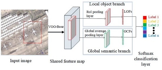
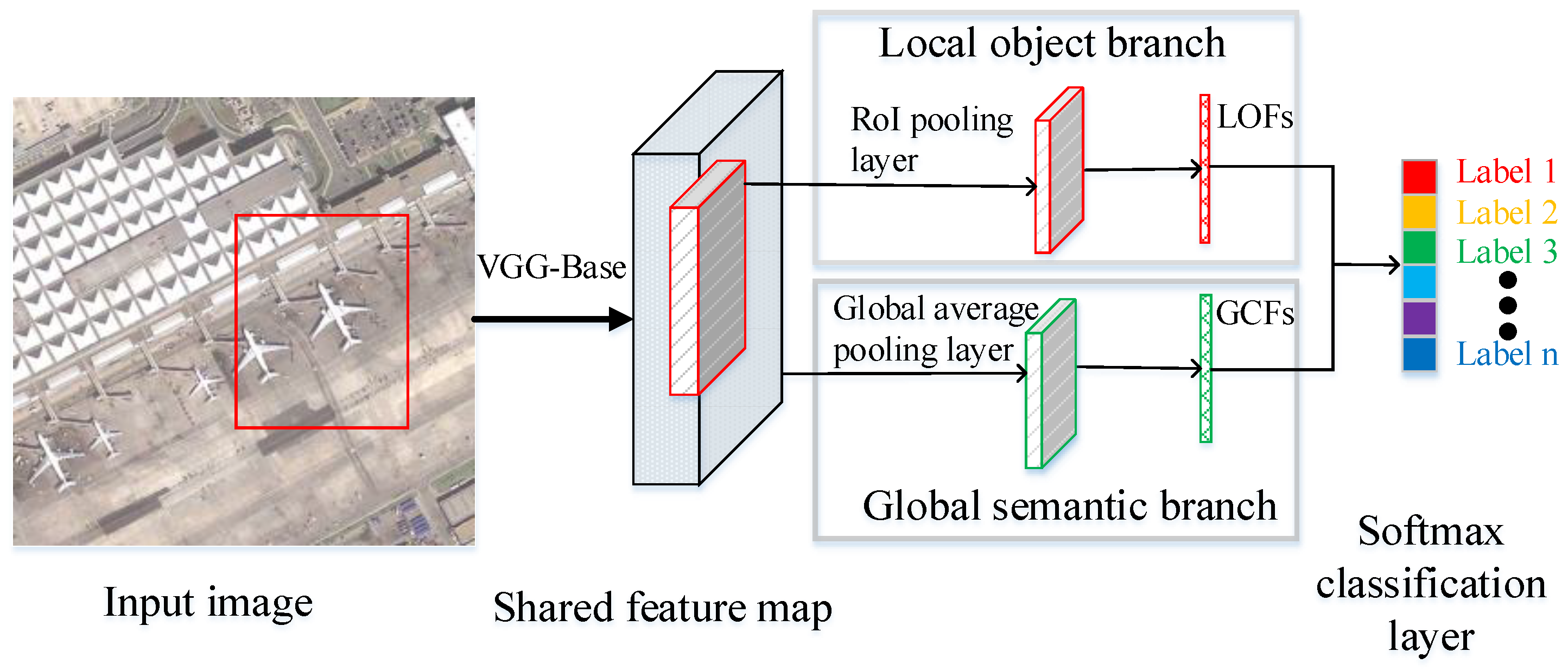
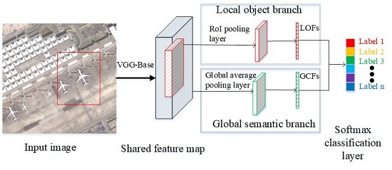
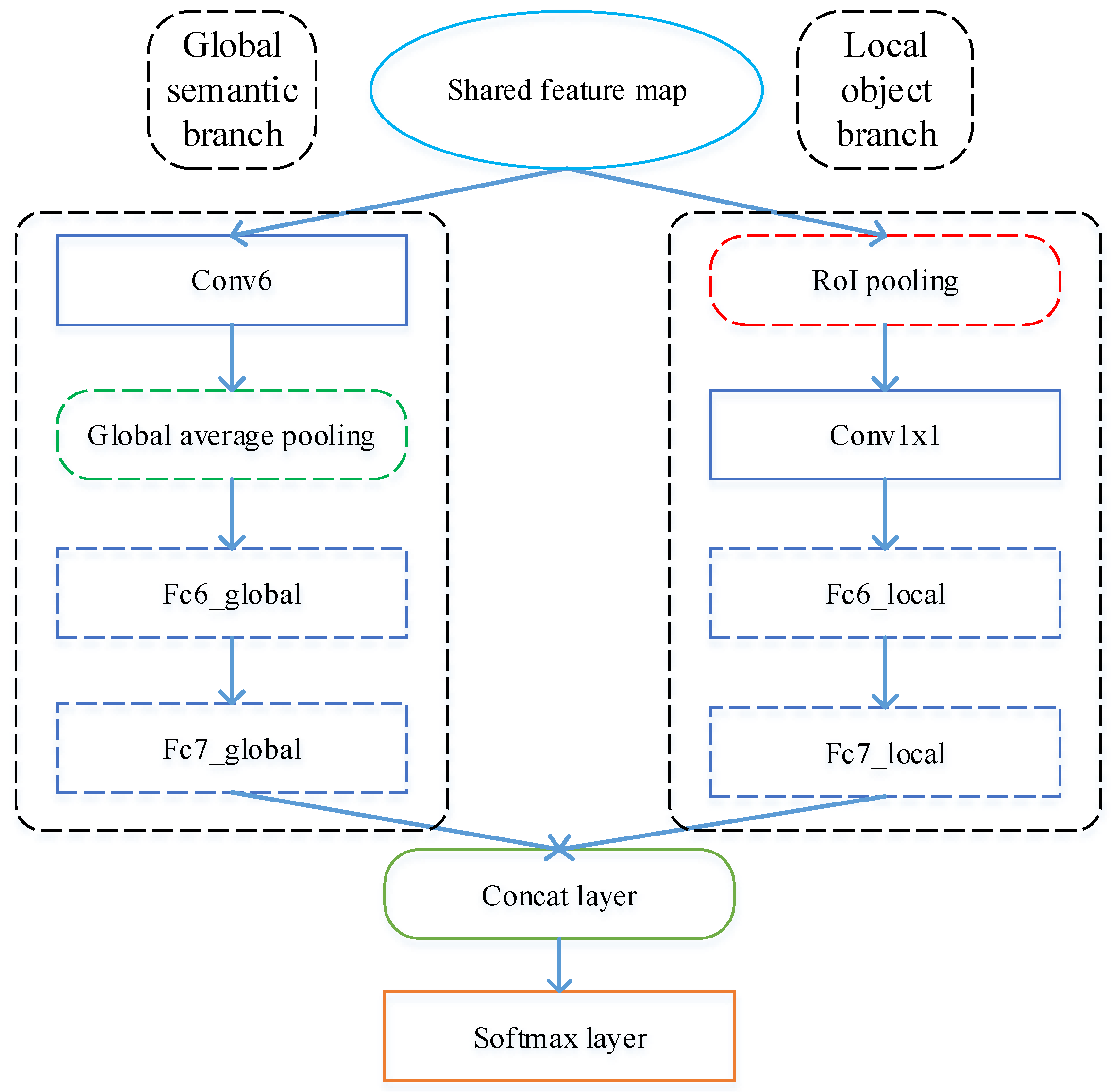
To address the issue that many previous CNN-based methods in scene classification justly extract the global feature from a single scene image and ignore LOFs that would help to infer the scene, we propose a novel two-branch, end-to-end CNN model to capture both GCFs and LOFs simultaneously.

(2)

Our network supports input of arbitrary size by using global average pooling layer and RoI pooling layer. Compared with methods that require fixed-size input images produced by resizing the scene image to a certain scale or cropping fixed-size patches from image, our method can extract more applicable features from the original-scale image.

(3)

By integrating GCFs and LOFs, our method can obtain superior performance compared with the state-of-the-art results from three challenging datasets.

The remainder of this paper is organized as follows. In Section 2, we illustrate the materials and the proposed architecture in detail. Section 3 introduces the experimental results of the proposed scene classification method. Section 4 discusses the influence of several factors. Section 5 concludes the paper with a summary of our method.

2. Materials and Methods

2.1. Datasets

AID [5] is an available large-scale aerial image dataset. It contains 10,000 aerial images with a fixed size of 600 × 600 pixels and is divided into 30 classes. Figure 2 shows representative images of each class, that is, airport, bare land, baseball field, beach, bridge, center, church, commercial, dense residential, desert, farm land, forest, industrial, meadow, medium residential, mountain, park, parking, playground, pond, port, railway station, resort, river, school, sparse residential, square, stadium, storage tanks, viaduct. The numbers of images vary from 220 to 420 with different aerial scene classes. The spatial resolution changes from about 8 m to about 0.5 m. With higher intra-class variations and smaller inter-class dissimilarity, AID has become an eye-catching and challenging dataset.

UC-Merced [15] dataset contains 2100 aerial scene images with regions of 256 × 256 pixels with a pixel resolution of 30 cm in the red green blue (RGB) color space. And the images are manually labeled into 21 categories, as shown in Figure 3 , including agricultural, airplane, baseball diamond, beach, buildings, chaparral, dense residential, forest, freeway, golf course, harbor, intersection, medium density residential, mobile home park, overpass, parking lot, river, runway, sparse residential, storage tanks, and tennis courts. This dataset has many highly overlapping classes, such as medium residual, sparse residual and dense residual, and only differ in the density of structures, which make the dataset difficult for classification.

RSSCN7 [47] dataset contains 2800 remote sensing images collected from the Google Earth and is divided into 7 scene categories, that is, grassland, forest, farmland, parking lot, residential region, industrial region, river and lake. Each category consists of 400 images with a size of 400 × 400 pixels. Classification for this dataset is challenging because the images are sampled at four different scales with different imaging angles, as shown in Figure 4.

2.2. Methods

In this section, we first introduce the overall architecture; then the VGG-Base and the branches extracting GCFs and LOFs is detailed separately.

2.2.1. Overall Architecture

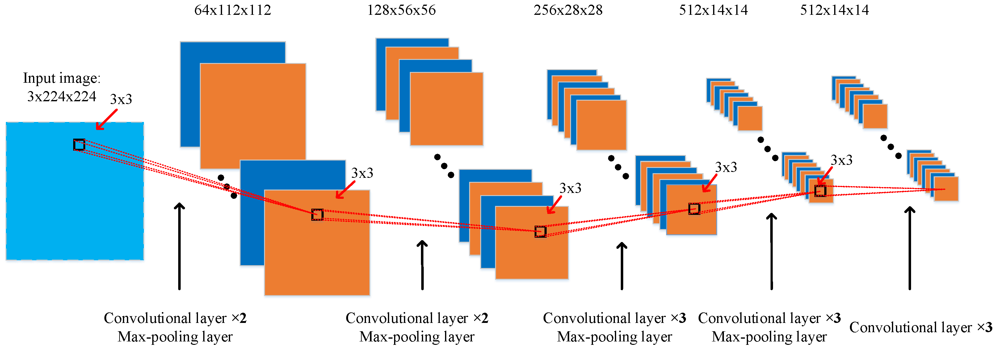
As illustrated in Figure 5, our proposed architecture can be mainly divided into three parts: VGG-Base, GSB and LOB. The processing flow of our architecture is as follows. Firstly, an image randomly selected from the dataset is fed into the VGG-Base without cropping and resizing operation. Compared with methods that require fixed-size input images, therefore resizing images to a certain scale or cropping fixed-size patches, our method can extract more applicable features from original-scale images. Taking an image as input, the VGG-Base network, which is the backbone of our framework, maps the image into a shared feature map followed by two branches. Then, according to the given position of the RoI, that is, the red rectangle in the input image, LOFs are produced by the RoI pooling layer in LOB. GCFs can be generated via the global average pooling layer in the GSB. Finally, both features are concatenated and fed into a softmax classification layer. The GSB can capture the global environmental background of the whole image, and the LOB extracts LOFs from the RoI. By integrating LOFs and GCFs, our method can generate a more discriminative feature representation than that produced by only extracting one feature, as demonstrated in Section 3.3. It is worth noting that our architecture supports input of arbitrary size because the RoI pooling layer and global average pooling layer can map arbitrary-size input to fixed-size output.

2.2.2. VGG-Base

As shown in Figure 6, the VGG-Base network is structured as a series of layers, including convolutional layers and pooling layers. Compared with traditional feature extraction methods, such as SIFT, convolutional layers can automatically extract features from data. Following convolutional layers, max pooling layers, which compute the maximum of a local patch of units in one feature map, are added to reduce the dimension of representation and create invariance to small translations or rotations. Our VGG-Base network is modified from VGG16 [31], which has shown excellent performance in many computer vision tasks. As shown in Figure 6, “3 × 3” means the kernel size of convolutional layer. “3 × 224 × 224” means that the channel of input image is 3, and the size is 224 × 224. Particularly, all 13 convolutional layers contained in VGG-Base adapt 3 × 3 kernel size. VGG16 contains 13 convolutional layers, 5 max-pooling layers, and 3 fully connected layers; however we remove the 3 fully-connected layers and the last max-pooling layer in our VGG-Base network. Specifically, as discussed in [34], the requirement of fixed-size images only comes from fully-connected layers. Thus, the three fully connected layers in VGG16 are novelly removed with the consideration of any size input of our network. Furthermore, the existing five max-pooling layers in VGG16 make the size of the shared feature map $\frac{1}{32}$ that of the input image. To avoid the difficulty of extracting LOFs from a small feature map, we also remove the last max-pooling layer.

2.2.3. Global Semantic Branch

As shown in Figure 7, the input of the GSB is the whole shared feature map with global-context information. Then, the shared feature map goes through the following Conv6, global average pooling, Fc6_global and Fc7_global layers in turn. Finally, GCFs can be obtained with the dimension of 2048. The detailed parameters of these layers are shown in

Table 1. The detailed parameters of global semantic branch (GSB), supposing the size of the shared feature map is H × W × 512; “$\lfloor .\rfloor$” refers to ceiling operation, and “-” refers to no parameters.

Layer Name	Weights Shape	Bias Shape	Output Shape
Conv6	512 × 3 × 3 × 512	1 × 512	($\lfloor \frac{H-3}{2}\rfloor$ + 1) × ($\lfloor \frac{W-3}{2}\rfloor$ + 1) × 512
Global average pooling	-	-	1 × 1 × 512
Fc6_global	512 × 2048	1 × 2048	1 × 2048
Fc7_global	2048 × 2048	1 × 2048	1 × 2048

. Following the convolutional layers in VGG-Base, we add an extra convolutional layer named Conv6 to increase the depth of GSB and extract high-level global semantic features. This branch introduces a global average pooling layer, which has three main advantages. First, the global pooling layer further helps the integration of global information by taking the average of each feature map. Furthermore, it is more robust to spatial translations of the input. Second, this layer has no parameter to learn and needs few computations to process a large input feature map compared with the fully connected layer. Overfitting is reduced at this layer. Third, the global average pooling operation can map an input feature map with any size into a fixed-length vector. Therefore, our network is suitable for images of different sizes. Additionally, two fully connected layers are added into the GSB, consistently with the original VGG16 network. In particular, the neurons of the Fc6_global and Fc7_global layers are 2048 compared with 4096 in VGG16. The effect on the output of the fully connected layer is analyzed in Section 4.2.

2.2.4. Local-Object Branch

In order to more accurately extract the object features, we first need to know the location of the objects. However, for a given scene image, we lack prior knowledge about the location of a certain object. This means if the region in which the object would appear with a high probability can be prepared in advance, the object features could be more accurately extracted. Inspired by the success of object detection, to realize this purpose, the extraction of local-object feature includes two steps, which are object proposals production and object feature extraction according to the positions of given object proposals. As shown in Figure 7, the LOB modified from Fast r-cnn [33] has two inputs. One is the shared feature map, as for the GSB, and the other is a list of RoI positions, that is, the locations of object proposals. Moreover, each proposal is defined as a tuple (r, c, h, w) that specifies the RoI’s top-left location (r, c) and its height and width (h, w). The detailed parameters of this branch are shown in

Table 2. The detailed parameters of Local Object Branch. “n” refers to the number of object proposals, and “-” refers to no parameters.

Layer Name	Weights Shape	Bias Shape	Output Shape
RoI pooling	-	-	n × 7 × 7 × 512
Conv1 × 1	n × 1 × 1 × 512	1 × 512	7 × 7 × 12
Fc6_local	25,088 × 2048	1 × 2048	1 × 2048
Fc7_local	2048 × 2048	1 × 2048	1 × 2048

.

Object proposals production: In this paper, we use the EdgeBoxes [48] algorithm to quickly produce category-independent object proposals. Edges provide a sparse yet informative representation of an image. Thus, the number of contours that are wholly contained in a bounding box is indicative of the likelihood of the box containing an object. In the EdgeBoxes algorithm, by producing the initial edge map, clustering the neighboring similar edge pixels to form groups, and computing the affinities between groups, series of object proposals can be obtained with confidence scores. The confidence score for a proposal is computed by summing the edge strengths of all edge groups within the box and subtracting the strengths of edge groups that are part of a contour that straddles the box’s boundary. Finally, by ranking the object proposals’ scores, a list of RoI positions containing objects can be obtained. How the number of proposals affects the performance of our network is discussed in Section 4.1.

Objects feature extraction: We use the RoI pooling layer to efficiently extract objects feature according to the given position (r, c, h, w) of each proposal. The shared feature map is $\frac{1}{16}$ of the input image. As can be seen from Figure 5, the feature map finally input into LOB is cropped according to the location ($\frac{r}{16}$,$\frac{c}{16}$,$\frac{h}{16}$,$\frac{w}{16}$). Then the cropped feature map of each proposal is mapped into a fixed-size feature map by the RoI pooling layer. Supposing the cropped feature map has a size of a × a. In order to get the feature map of size b × b, RoI pooling is implemented as a sliding window pooling, where the window = $\lceil \frac{a}{b}\rceil$ and stride = $\lfloor \frac{a}{b}\rfloor$ with $\lceil .\rceil$ and $\lfloor .\rfloor$ denoting ceiling and floor operations, respectively. Unlike Fast r-cnn, which predicts the class and location of each proposal, we have merged each object proposal’s feature into a super feature space. We have also added an extra convolutional layer with a filter size of 1 × 1, named Conv1 × 1, in addition to the RoI pooling layer to increase the non-linear and generalization ability of the network. Moreover, with two more fully connected layers, the LOB can produce local-object features which have the same dimension as the final feature vector in the GSB.

By ignoring the redundant information around the RoI, the LOB can focus on the key objects supporting the scene reasoning. Additionally, RoI pooling can map a feature map with any size into a fixed-size feature map. This means that an image with any size can be directly fed into our network.

3. Results

3.1. Experimental Setup

3.1.1. Implementation Details

We utilized the open-source Caffe framework [49] to implement our proposed architecture. In the experiments, two training ratios are adopted for each dataset, following the work of [5,50,51] for a fair comparison. For the AID and RSSCN7 datasets, 50% and 20% of the samples are randomly selected as the training samples and the left for testing. For the UC-Merced dataset, we fixed the ratios of the number of training set to 80% and 50%, respectively. Data augmentation [44] is critical to generate sufficient data to train an effective model. Our augmentation operations mainly included rotating in four different orientations ($0^{\circ }$, ${90}^{\circ }$, ${180}^{\circ }$, ${270}^{\circ }$), left-right flipping, up-down flipping, and randomly adding the White Gaussian Noise. Hyper-parameters used for training were set as below. The base learning rate was set to ${10}^{-5}$. The step size and the maximum number of iterations were set as 30,000 and 100,000, respectively. For the stochastic gradient descent (SGD) optimization algorithm, the batch size was set to 1, the weight decay was set to 0.0005, and the momentum was set to 0.9. It is worth noting that our VGG-Base network is fine-tuned from the pre-trained VGG16 model on ImageNet, while the two branches are trained from scratch. In all experiments, the filter weights of both branches are initialized by Gaussion distribution with zero mean and unit variance. All the implementations were evaluated on the Ubuntu 14.04 operating system with one 3.8 GHz 6-core CPU and 128 GB memory. Additionally, a GTX 1080Ti graphics processing unit (GPU) was used to accelerate computing.

3.1.2. Evaluation Protocol

We report the overall accuracy and confusion matrix to compare with the state-of-the-art methods. The overall accuracy is defined as the number of correctly classified images divided by the total number of images. The confusion matrix is an informative table used for analyzing the errors and confusions between different scene classes, and it is obtained by counting each class of correct and incorrect classifications of the test images and accumulating the results in the table. To compute the overall accuracy, we randomly selected the training set according to the above training ratios and repeated it ten times to reduce the influence of the randomness to obtain mean and standard deviation of convincing overall accuracy. Additionally, the confusion matrix was obtained by fixing the ratio of the number of training sets of the AID dataset, UC-Merced dataset and RSSCN7 dataset to be 20%, 50%, 20%, respectively.

3.2. Experimental Results and Analysis

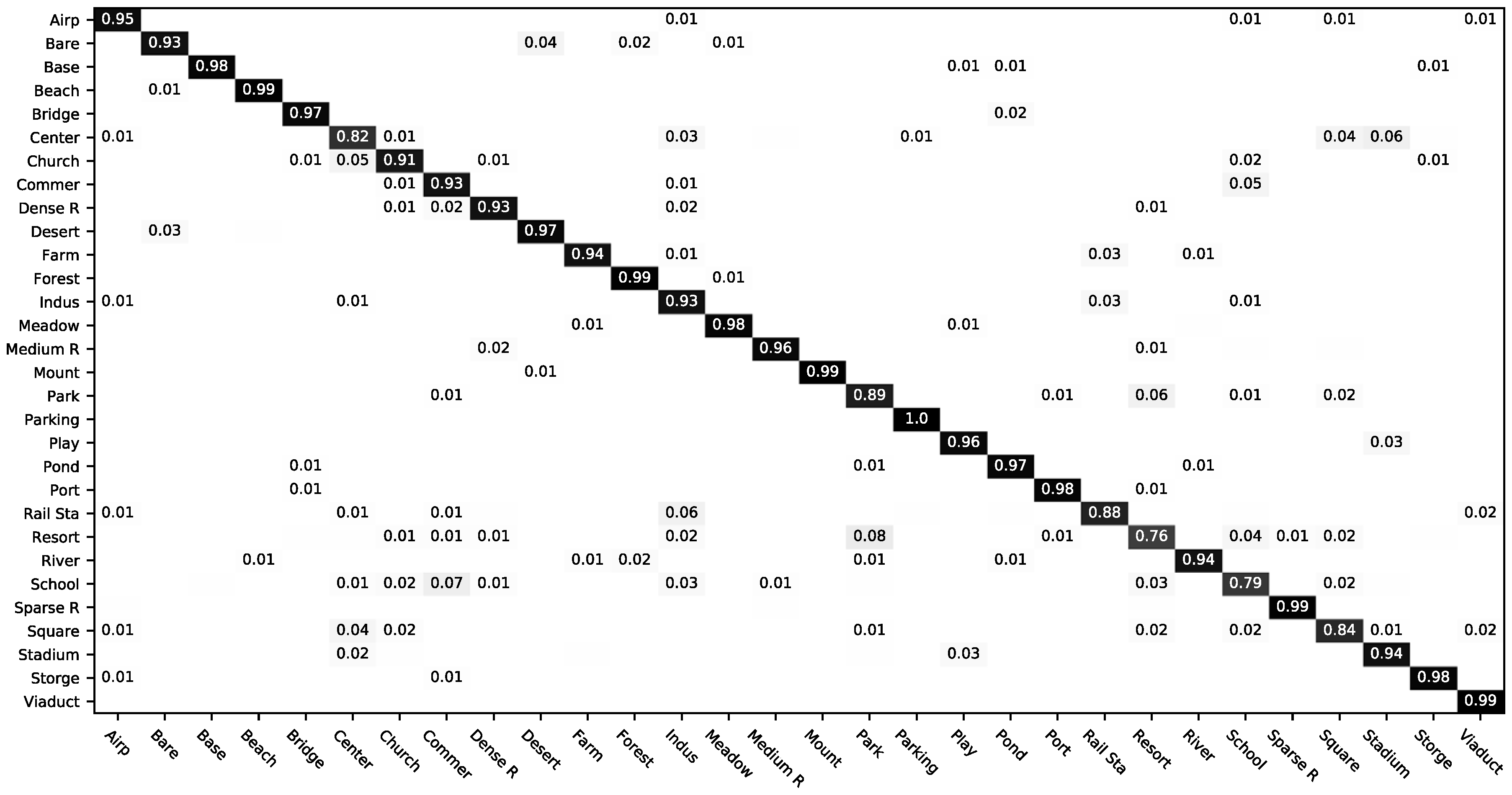
3.2.1. Classification of AID

A comparative evaluation against several state-of-the-art scene classification methods on the AID dataset is shown in

Table 3. Overall accuracy (%) and standard deviations of the proposed method and the comparison methods under the training ratios of 50% and 20% on the AID dataset.

Methods	50% Training Set	20% Trainging Set
CaffeNet [5]	89.53 ± 0.31	86.86 ± 0.47
GoogLeNet [5]	86.39 ± 0.55	83.44 ± 0.40
VGG16 [5]	89.64 ± 0.36	86.59 ± 0.29
salM${}^3$LBP-CLM [37]	89.76 ± 0.45	86.92 ± 0.35
TEX-Net-LF [50]	92.96 ± 0.18	90.87 ± 0.11
Fusion by addition [45]	91.87 ±0.36	-
Two-Stream Fusion [51]	94.58 ± 0.41	92.32 ± 0.41
Ours	96.85 ± 0.23	92.48 ± 0.38

. As can be seen from Table 3, our classification method, by fusing the GCFs and LOFs, achieved the highest overall accuracy of 96.85% and 92.81% using 50% and 20% training ratios, respectively. Worthy of mention is that our architecture outperformed the second-best model [51], which uses a feature fusion method to reconstruct global feature representation, with increases in the overall accuracy of 2.27% and 0.16%. The good performance of our method is mainly the results of the fusion of GCFs and LOFs.

Figure 8 shows the confusion matrix generated by the proposed method with the 20% training ratio. From the confusion matrix, we can see that almost 80% of the 30 categories achieved the classification accuracy of greater than 90%. Some types with small inter-class dissimilarity, such as dense residential (0.93), medium residential (0.96), and sparse residential (0.99), could also be accurately classified. However, the major confusions were between school and commercial, resort and park. As illustrated in Figure 2, school and commercial have the same image distribution, for example, clutter structures; resort and park have the analogous objects and image texture, for example, green belts and buildings. Thus, these classes were easily confused. Even so, our method achieved a substantial improvement for the difficult scene types compared with the accuracies (0.49, 0.6, 0.63, 0.65) of the same classes from the confusion matrix of [5], which directly used the deep learning image classification model. This result is possibly explained by the fact that the integration of GCFs and LOFs gives the ability to learn discriminative features. Particularly, for the scenes that are rich in obvious objects, such as airport, industry, and dense (medium, sparse) residential, our method can achieve higher accuracies by capturing the features of key objects when compared with the accuracies of [37]. For the scenes consisting of many textures, such as desert and bare land, our method can also achieve comparable performance. Thus, the fusion of the GCFs and LOFs can achieve accurate scene reasoning.

3.2.2. Classification of UC-Merced

In order to further measure the scene classification performance of our approach, we also compared the classification accuracies with several state-of-the-art methods on the UC-Merced dataset. The final accuracies certify the effectiveness of our method, as shown in

Table 4. Overall accuracy (%) and standard deviations of the proposed method and the comparison methods under the training ratios of 80% and 50% on the UC-Merced dataset.

Methods	80% Training Set	50% Training Set
SCK [15]	72.52	-
SPCK [21]	73.14	-
BoVW [15]	76.81	-
BoVW + SCK [15]	77.71	-
SIFT + SC [38]	81.67	-
MCMI [13]	88.20	-
Unsupervised feature learning [38]	81.67 ± 1.23	-
Gradient boosting CNNs [39]	94.53	-
MS-CLBP + FV [12]	93.00 ± 1.20	88.76 ± 0.79
LGF [52]	95.48	-
SSF-AlexNet [40]	92.43	-
Multifeature concatenation [7]	92.38 ± 0.62	-
CaffeNet [5]	95.02 ± 0.81	93.98 ± 0.67
GoogLeNet [5]	94.31 ± 0.89	92.70 ± 0.60
VGG16 [5]	95.21 ± 1.20	94.14 ± 0.69
Fine-tuned GoogLeNet [42]	97.10	-
Deep CNN Transfer [44]	98.49	-
salM${}^3$LBP-CLM [37]	95.75 ± 0.80	94.21 ± 0.75
TEX-Net-LF [50]	96.62 ± 0.49	95.89 ± 0.37
Fusion by addition [45]	97.42 ± 1.79	-
Two-Stream Fusion [51]	98.02 ± 1.03	96.97 ± 0.75
Ours	99 ± 0.35	97.37 ± 0.44

. Our method generated state-of-the-art performance again with accuracies of 99%, 97.37% by using 80%, 50% labeled samples per class, respectively. Our proposed method produced better results than the second-highest accuracy of 98.49% reported in [44] on this dataset, which was implemented by aggregating multi-scale dense features to generate the global image representations. By capturing the key LOFs, which are ignored in [44], the discriminative and powerful image representations can be captured in our architecture. Compared with the LGF method introduced in [52], which also combines local and global features, our method is superior. Zhou et al. extracted local and global features by SIFT [6] and MS-CLBP [12], which are hand-crafted descriptors. Our experimental results demonstrate the superior performance of CNNs can be generated, compared to the hand-crafted descriptor. Figure 9 shows the confusion matrix on this dataset. It is interesting that most of the scene types could achieve an accuracy of over 0.96, yet dense residential has an accuracy of 0.74. We believe that there is major confusion between dense residential and medium residential. As we can see in Figure 3, the scenes of dense residential and medium residential have similar spatial distribution and scale of buildings. Thus, it is likely that dense residential was misclassified as medium residential.

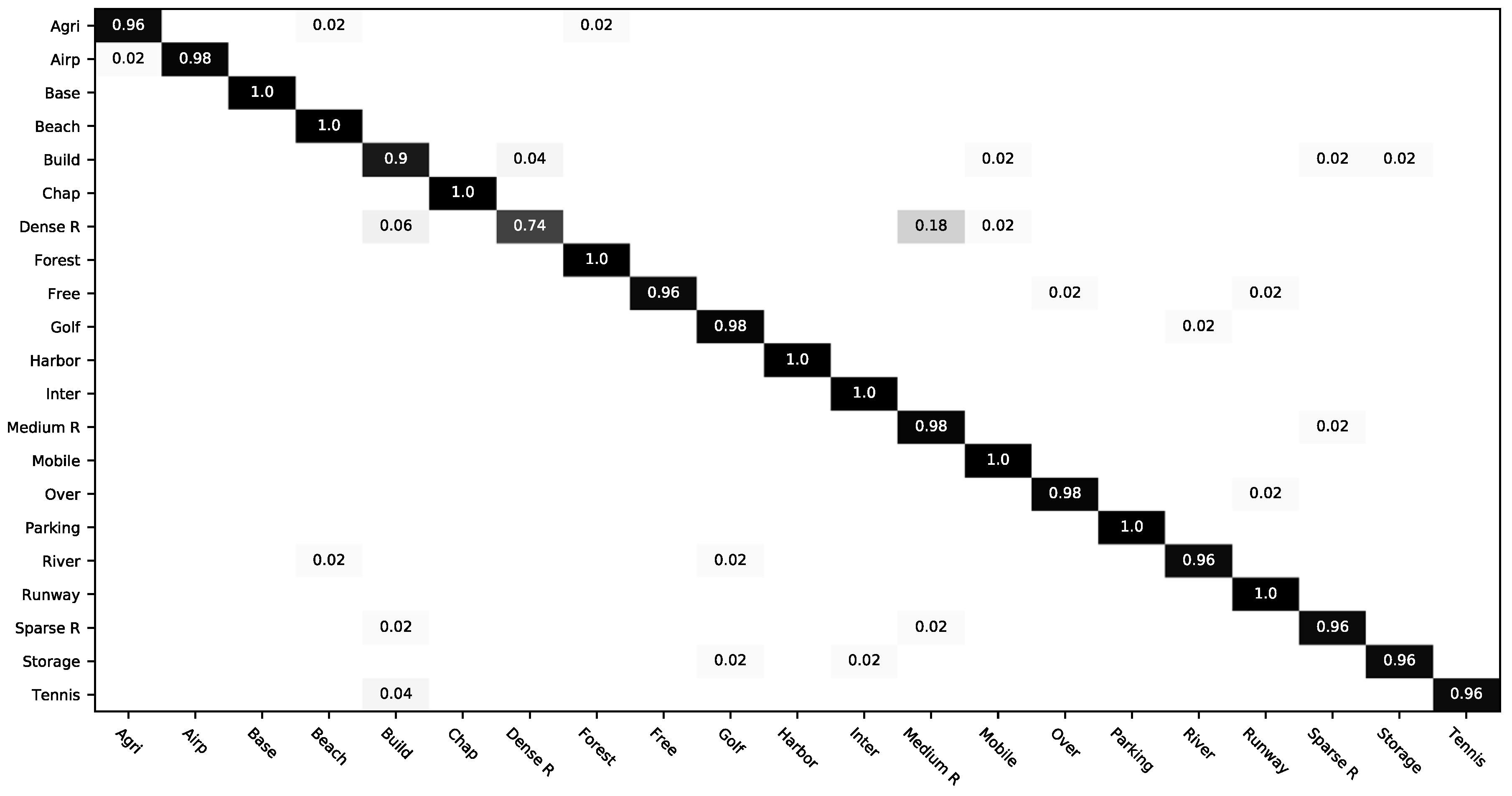
3.2.3. Classification of RSSCN7

Because the images were collected from four different scales and angles in RSSCN7 dataset, the proposed approach was also carried out on this dataset.

Table 5. Overall Accuracy (%) and standard deviations of the proposed method and the comparison methods under the training ratios of 50% and 20% on the RSSCN7 dataset.

Methods	50% Training Set	20% Training Set
CaffeNet [5]	88.25 ± 0.62	85.57 ± 0.95
GoogLeNet [5]	85.84 ± 0.92	82.55 ± 1.11
VGG16 [5]	87.18 ± 0.94	83.98 ± 0.87
DBN [47]	77	-
HHCV [20]	84.7 ± 0.7	-
Deep Filter Banks [41]	90.4 ± 0.6	-
Ours	95.59 ± 0.49	92.47 ± 0.29

shows the classification performance comparison of our architecture compared to the state-of-the-art methods. Our method outperformed all other methods with the overall accuracies of 95.59% and 92.47% using 50% and 20% training ratios, respectively. Figure 10 shows the confusion matrix. From the confusion matrix, we can conclude that six types of the seven classes were accurately classified by our method. Only one class industry had major confusion with the class parking. In order to find out the reason of this, the images’ names in the industry class, which were wrongly classified, and the probabilities of the classifying industry into parking class are listed, as shown in Figure 11. We can easily see that these three industry images were so similar to the scenes of parking that a human could not accurately classify them. Because of the existing major confusion between these two categories, our method had superior performance in inferring the scene for this dataset than the state-of-the-art methods. Specifically, the overall accuracies of class residential and class parking were (0.96, 0.93). Compared with the accuracies of the same classes from the confusion matrix in [5,41], which are respectively (0.84, 0.83) and (0.95, 0.89), the performance was greatly improved by integrating the global environment information and local-object features in our method. Generally, the experimental results demonstrate the effectiveness of our approach in recognizing the complicated remote scene images.

3.3. Ablation Study

To evaluate the effectiveness of our proposed method, ablation experiments were conducted by using only global semantic branch (GSB) or local object branch (LOB) on both the AID and UC-Merced datasets. Additionally, we fine-tuned the pre-trained VGG16 model [31] on the AID and UC-Merced datasets by using the default configurations as the baseline. All experimental results are shown in

Table 6. Overall Accuracy (%) of different methods on AID and UC-Merced. “Baseline” refers to the method using original VGG16 model, “Local” refers to the method using only local-objects features, “Global” refers to the method only using global context feature, “Global + Local” refers to the proposed method fusing both global-context and local-object features.

Methods	AID		UC-Merced
	50% Training Set	20% Training Set	80% Training Set	50% Training Set
Baseline	94.08	91.25	96.90	95.33
Local	87.44	86.34	95.47	94.76
Global	95.04	92.25	98.09	96.28
Global + Local	96.85	92.48	99	97.37

, and the following can be seen from the results.

(1)

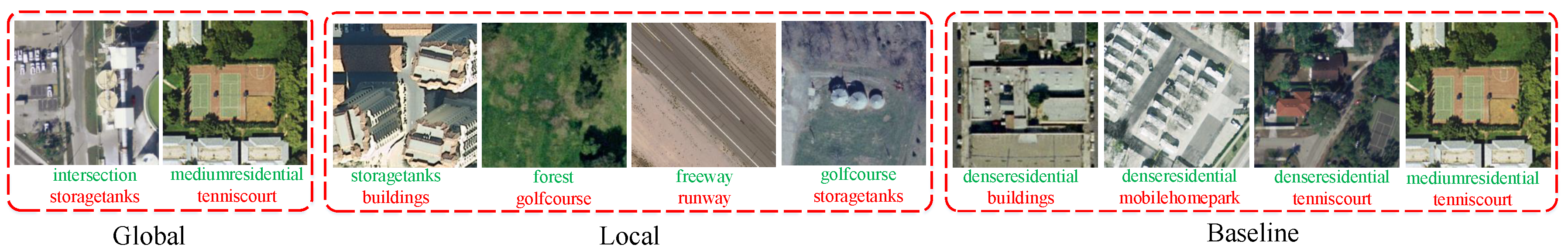
Results from LOB are the worst, which was because the LOB can only extract local-object features without paying attention to GCFs. It is not reliable for classifying a scene by only focusing on part of the image.

(2)

The method using only the GSB works better than the baseline method. We think there are two reasons. One is that our GSB architecture introduces a global average pooling layer and is more applicable than VGG16 to extract global features by taking the average of each feature map. Another reason is that the resize operation in the original VGG16 network makes the objects smaller and makes it harder to extract features.

(3)

Our proposed method achieved the best performance compared to only using one branch or baseline method, which was a result of combining both GCFs and LOFs. The LOB is designed to describe objects in RoIs, while the GSB focuses on extracting GCFs. Therefore, a collaborative representation of the fusion of GCFs and LOFs can generate superior performance.

In addition, to further prove the practicability of our method, we present a few examples showing that the baseline method and method using only global or local feature cannot generate correct classifications while our proposed method can. As illustrated in Figure 12, the class of storagetanks in the left block was misclassified as intersection, because the GSB only focuses on its global environment and ignores important local objects such as tanks. The category of tenniscourt was confused with the mediumresidential category when using either the GSB or baseline method, as they pay more attention to the global structure while ignoring the vital local object tenniscourt. Additionally, failure cases in the middle block, such as runway being misclassified as freeway and building being misclassified as storagetanks, demonstrate that the LOB only focuses on local objects and ignores the global structure. These examples demonstrate that using only one branch or baseline cannot achieve promising results, while our proposed collaborative representation of the fusion of GCFs and LOFs is more effective in scene classification.

4. Discussion

In this section, three factors, the number of proposals, the number of model weights, and the kernel size of the RoI pooling, were tested to analyze how these factors affect classification accuracy. In all experiments, 80% of each class’ images in the UC-Merced dataset and a 50% training ratio in the AID dataset were chosen for the analysis of the above factors.

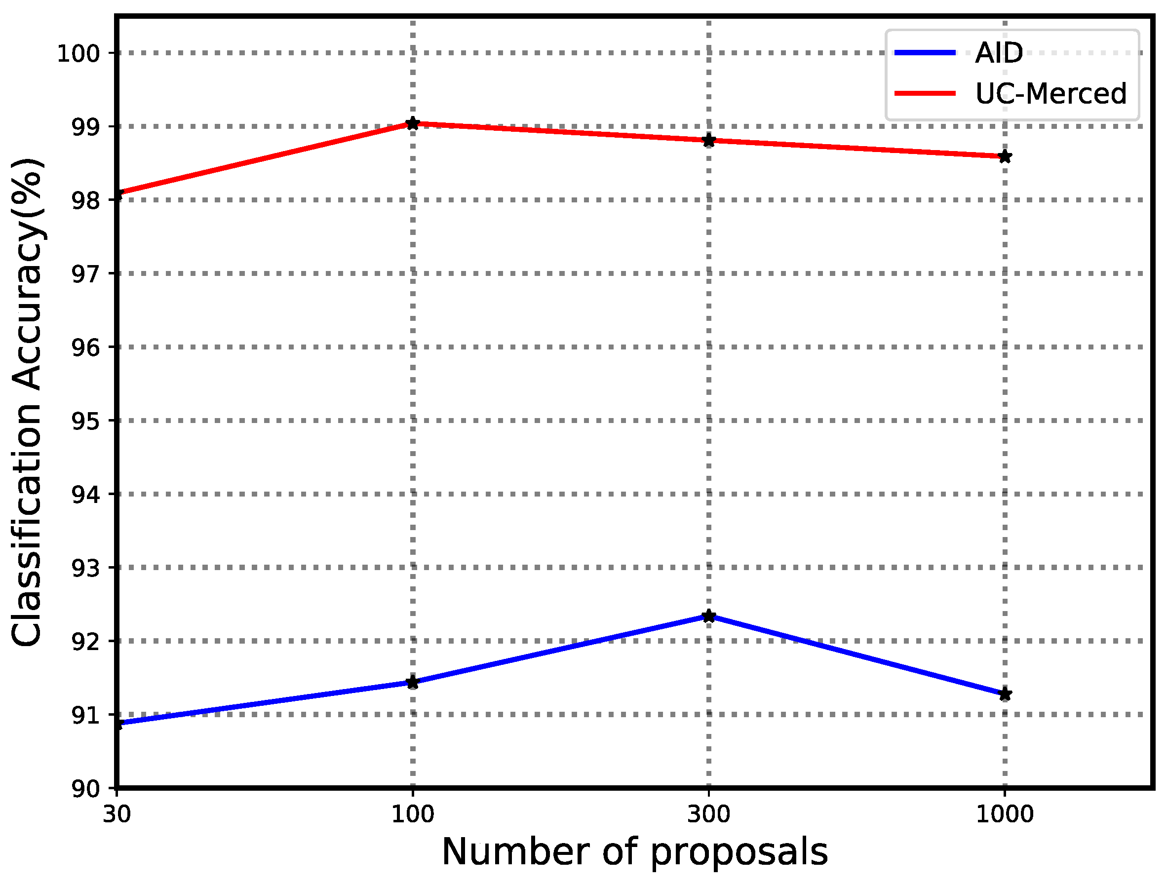
4.1. Evaluation of Number of Proposals

In our method, the object proposals are generated by ranking the confidence score of each proposal. Additionally, for n object proposals, we concatenated the local-object feature extracted from each object proposal into a super semantic feature space. Thus, the number of object proposals would influence the final classification accuracy. The number of proposals was varied as follows: n = {30, 100, 300, 1000}, and the other parameters were kept the same. From Figure 13, the classification accuracies firstly increase and then decrease with the increasing of the number of proposals. The changing trend for both datasets could be explained by the object proposals with high scores have a large probability to contain objects, while the low-score object proposals may justly contain the textual information without object features. Hence, a smaller proposal number leads to the local-object features with insufficient information on objects, and a greater proposal number leads to redundant information that mainly includes similar textual cue. It is interesting that the best accuracy was obtained for different proposal number for the two datasets, that is, 300 proposals for AID and 100 proposals for UC-Merced. We believe there are two main reasons for this phenomenon. One is that the scale of AID dataset is much larger than UC-Merced, and therefore more robust and discriminative feature needed to be extracted. The other is that the number of objects in the scene is different. For example, the object numbers in same scenes in both datasets, e.g., 3 vs. 3, 9 vs. 7, 15 vs. 13 in Figure 2 and Figure 3, are clearly different. In particular, the airport class in the AID dataset contains many airplanes, while the airplane class in UC-Merced dataset contains only a few airplanes. This indicates that the model trained on AID dataset needed more object proposals to capture LOFs for scene reasoning.

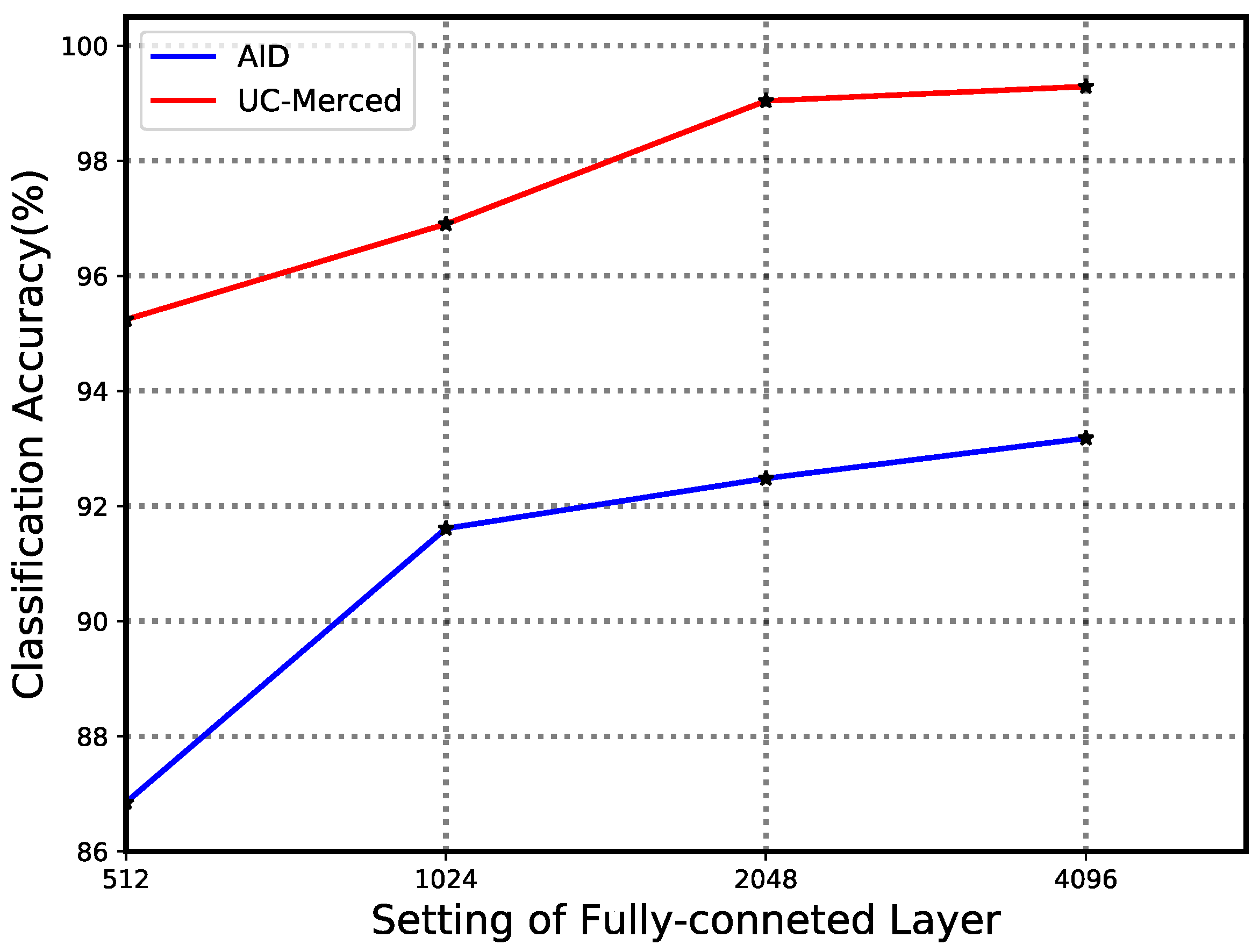
4.2. Evaluation of Number of Model Weights

Commonly, the number of model weights influences the performance of a CNN model. The model weights mainly result from fully connected layers because of the connecting of every neuron from one layer to another. To reduce the number of model weights, in principle, the number of neurons of a fully connected layer should be decreased. However, the performance of a CNN model would be decreased due to the reduction in the number of model weights. Therefore, to trade-off the performance and model weights, the number of outputs of fully connected layers were tested by separately by setting the number of neurons of FC6_global, FC7_global, FC6_local, and FC7_local (as shown in Figure 7) as {512, 1024, 2048, 4096}, and the other parameters were kept the same. From Figure 14, when the neurons of a fully connected layer increased from 512 to 4096, the classification accuracy of both datasets improved. The size of the models were {123, 181, 312, 623} MB. However, the size of VGG16 model was 553 MB. It is interesting that when the model size was 312 MB, the classification accuracies of our method were 92.48% and 99.04% in the AID and UC-Merced datasets, respectively. It is very convincing that the architecture integrating the GCFs and LOFs effectively improves the scene classification of remote-sensing images, as the number of model weights is smaller than the original VGG16. The accuracies reported in Section 3 were obtained by setting the neurons as 2048.

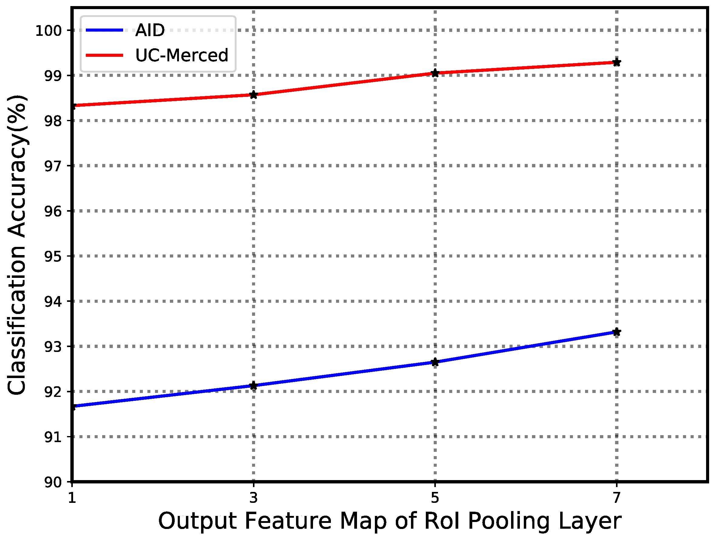
4.3. Evaluation of Scale of RoI Pooling Kernel

The RoI pooling layer is used for extracting the LOFs by sliding window with window = $\lceil \frac{a}{b}\rceil$ and stride = $\lfloor \frac{a}{b}\rfloor$ , where a means the size of input feature map, and b is the size of the output feature map in the layer. Commonly, the objects in remote-sensing scenes are usually small and hard to detect. Thus, a moderate window size is necessary for LOFs extraction. Four different window sizes were tested to analyze how these affected classification accuracy by setting the size of output feature map as {1 × 1, 3 × 3, 5 × 5, 7 × 7}. For the same size of input feature map, the window size decreased when the size of output feature map increased. As can be seen from Figure 15, the classification accuracy improved as the size of output feature map increased , that is, as the window size decreased. This comparison between different window sizes suggests that a smaller window size could capture small local-object information helpful to infer scenes. The accuracies reported in Section 3 were obtained by setting the output feature map of RoI pooling layer as 7 × 7.

5. Conclusions

In this paper, to solve the problem of difficulty in extracting both the global context and small local objects in conventional remote-sensing scene classification methods, we propose a novel end-to-end scene classification architecture that consists of two branches. By integrating global context features (GCFs) extracted in global semantic branch (GSB) and local-object-level features (LOFs) extracted from local object branch (LOB), our network can learn robust and abstract feature representations of scene image. To address the problem of fixed-size inputs of traditional CNN models, which causes the objects in the original scene to be smaller and harder to detect, our architecture supports input of any size for taking full advantage of objects’ feature.

To test the performance of our method, experiments were performed on the challenging AID, UC-Merced, and RSSCN7 datasets. Extensive experimental results consistently showed that our architecture outperforms the current state-of-the-art methods. Particularly, when compared with the methods that use CNNs as the global feature extractor, our method, integrating the LOFs and GCFs, obtained the best accuracy. In the future work, we will conduct a multi-task network for simultaneously carrying out the object detection and scene classification of remote-sensing images.

References

1. Hu, Q.; Wu, W.; Xia, T.; Yu, Q.; Yang, P.; Li, Z.; Song, Q. Exploring the use of Google Earth imagery and object-based methods in land use/cover mapping. Remote Sens. 2013, 5, 6026–6042. [Google Scholar] [CrossRef]
2. Zhang, L.; Zhang, L.; Du, B. Deep learning for remote sensing data: A technical tutorial on the state of the art. IEEE Geosci. Remote Sens. Mag. 2016, 4, 22–40. [Google Scholar] [CrossRef]
3. Yang, W.; Yin, X.; Xia, G.S. Learning high-level features for satellite image classification with limited labeled samples. IEEE Trans. Geosci. Remote Sens. 2015, 53, 4472–4482. [Google Scholar] [CrossRef]
4. Shao, W.; Yang, W.; Xia, G.S. Extreme value theory-based calibration for the fusion of multiple features in high-resolution satellite scene classification. Int. J. Remote Sens. 2013, 34, 8588–8602. [Google Scholar] [CrossRef]
5. Xia, G.S.; Hu, J.; Hu, F.; Shi, B.; Bai, X.; Zhang, L.; Lu, X. AID: A benchmark data set for performance evaluation of aerial scene classification. IEEE Trans. Geosci. Remote Sens. 2017, 55, 3965–3981. [Google Scholar] [CrossRef]
6. Lowe, D.G. Distinctive image features from scale-invariant keypoints. Int. J. Comput. Vis. 2004, 60, 91–110. [Google Scholar] [CrossRef]
7. Shao, W.; Yang, W.; Xia, G.S.; Liu, G. A Hierarchical Scheme of Multiple Feature Fusion for High-Resolution Satellite Scene Categorization. In Proceedings of the International Conference on Computer Vision Systems, St. Petersburg, Russia, 16–18 July 2013; Springer: Berlin/Heidelberg, Germany, 2013; pp. 324–333. [Google Scholar]
8. Yang, Y.; Newsam, S. Comparing SIFT descriptors and Gabor texture features for classification of remote sensed imagery. In Proceedings of the 15th IEEE International Conference on Image Processing (ICIP), San Diego, CA, USA, 12–15 October 2008; pp. 1852–1855. [Google Scholar]
9. Dos Santos, J.A.; Penatti, O.A.B.; da Silva Torres, R. Evaluating the Potential of Texture and Color Descriptors for Remote Sensing Image Retrieval and Classification. In Proceedings of the VISAPP, Angers, France, 17–21 May 2010; pp. 203–208. [Google Scholar]
10. Swain, M.J.; Ballard, D.H. Color indexing. Int. J. Comput. Vis. 1991, 7, 11–32. [Google Scholar] [CrossRef]
11. Ojala, T.; Pietikainen, M.; Maenpaa, T. Multiresolution gray-scale and rotation invariant texture classification with local binary patterns. IEEE Trans. Pattern Anal. Mach. Intell. 2002, 24, 971–987. [Google Scholar] [CrossRef]
12. Chen, C.; Zhang, B.; Su, H.; Li, W.; Wang, L. Land-use scene classification using multi-scale completed local binary patterns. Signal Image Video Process. 2016, 10, 745–752. [Google Scholar] [CrossRef]
13. Ren, J.; Jiang, X.; Yuan, J. Learning LBP structure by maximizing the conditional mutual information. Pattern Recognit. 2015, 48, 3180–3190. [Google Scholar] [CrossRef]
14. Luo, B.; Jiang, S.; Zhang, L. Indexing of remote sensing images with different resolutions by multiple features. IEEE J. Sel. Top. Appl. Earth Obs. Remote Sens. 2013, 6, 1899–1912. [Google Scholar] [CrossRef]
15. Yang, Y.; Newsam, S. Bag-of-visual-words and spatial extensions for land-use classification. In Proceedings of the 18th SIGSPATIAL International Conference on Advances in Geographic Information Systems, San Jose, CA, USA, 3–5 November 2010; pp. 270–279. [Google Scholar]
16. Chen, S.; Tian, Y.L. Pyramid of spatial relatons for scene-level land use classification. IEEE Trans. Geosci. Remote Sens. 2015, 53, 1947–1957. [Google Scholar] [CrossRef]
17. Zhou, L.; Zhou, Z.; Hu, D. Scene classification using a multi-resolution bag-of-features model. Pattern Recognit. 2013, 46, 424–433. [Google Scholar] [CrossRef]
18. Zhao, B.; Zhong, Y.; Zhang, L.; Huang, B. The fisher kernel coding framework for high spatial resolution scene classification. Remote Sens. 2016, 8, 157. [Google Scholar] [CrossRef]
19. Zhao, B.; Zhong, Y.; Xia, G.S.; Zhang, L. Dirichlet-derived multiple topic scene classification model for high spatial resolution remote sensing imagery. IEEE Trans. Geosci. Remote Sens. 2016, 54, 2108–2123. [Google Scholar] [CrossRef]
20. Wu, H.; Liu, B.; Su, W.; Zhang, W.; Sun, J. Hierarchical coding vectors for scene level land-use classification. Remote Sens. 2016, 8, 436. [Google Scholar] [CrossRef]
21. Yang, Y.; Newsam, S. Spatial pyramid co-occurrence for image classification. In Proceedings of the IEEE International Conference on Computer Vision, Barcelona, Spain, 6–13 November 2011; pp. 1465–1472. [Google Scholar]
22. Zhao, L.; Tang, P.; Huo, L. A 2-D wavelet decomposition-based bag-of-visual-words model for land-use scene classification. Int. J. Remote Sens. 2014, 35, 2296–2310. [Google Scholar]
23. Zhao, L.; Tang, P.; Huo, L. Land-use scene classification using a concentric circle-structured multiscale bag-of-visual-words model. IEEE J. Sel. Top. Appl. Earth Obs. Remote Sens. 2014, 7, 4620–4631. [Google Scholar] [CrossRef]
24. Lazebnik, S.; Schmid, C.; Ponce, J. Beyond bags of features: Spatial pyramid matching for recognizing natural scene categories. In Proceedings of the IEEE Conference on Computer Vision and Pattern Recognition, New York, NY, USA, 17–22 June 2006; pp. 2169–2178. [Google Scholar]
25. Blei, D.M.; Ng, A.Y.; Jordan, M.I. Latent dirichlet allocation. J. Mach. Learn. Res. 2003, 3, 993–1022. [Google Scholar]
26. Wang, Q.; Meng, Z.; Li, X. Locality adaptive discriminant analysis for spectral-spatial classification of hyperspectral images. IEEE Geosci. Remote Sens. Lett. 2017, 14, 2077–2081. [Google Scholar] [CrossRef]
27. Bosch, A.; Zisserman, A.; Munoz, X. Scene Classification via pLSA. In Proceedings of the European Conference on Computer Vision (ECCV), Graz, Austria, 7–13 May 2006; Springer: Berlin/Heidelberg, Germany, 2006; pp. 517–530. [Google Scholar]
28. Wang, Q.; Wan, J.; Yuan, Y. Deep metric learning for crowdedness regression. IEEE Trans. Circ. Syst. Video Technol. 2017. [Google Scholar] [CrossRef]
29. Zhu, H.; Vial, R.; Lu, S.; Peng, X.; Fu, H.; Tian, Y.; Cao, X. YoTube: Searching Action Proposal via Recurrent and Static Regression Networks. IEEE Trans. Image Process. 2018, 27, 2609–2622. [Google Scholar] [CrossRef] [PubMed]
30. Krizhevsky, A.; Sutskever, I.; Hinton, G.E. ImageNet classification with deep convolutional neural networks. In Proceedings of the 26th International Conference on Neural Information Processing Systems, Lake Tahoe, NY, USA, 3–8 December 2012; pp. 1097–1105. [Google Scholar]
31. Simonyan, K.; Zisserman, A. Very deep convolutional networks for large-scale image recognition. In Proceedings of the International Conference on Learning Representations, San Diego, CA, USA, 7–9 May 2015. [Google Scholar]
32. Szegedy, C.; Liu, W.; Jia, Y.; Sermanet, P.; Reed, S.; Anguelov, D. Going deeper with convolutions. In Proceedings of the IEEE Conference on Computer Vision and Pattern Recognition (CVPR), Boston, MA, USA, 11–12 June 2015; pp. 1–9. [Google Scholar]
33. Girshick, R. Fast r-cnn. arXiv, 2015; arXiv:1504.08083. [Google Scholar]
34. He, K.; Zhang, X.; Ren, S.; Sun, J. Spatial Pyramid Pooling in Deep Convolutional Networks for Visual Recognition. In Proceedings of the European Conference on Computer Vision (ECCV), Zurich, Switzerland, 6–12 September 2014; Springer: Cham, Swizerland, 2014; pp. 346–361. [Google Scholar]
35. Zhou, B.; Lapedriza, A.; Xiao, J.; Torralba, A.; Oliva, A. Learning deep features for scene recognition using places database. In Proceedings of Advances in Neural Information Processing Systems, Montreal, QC, Canada, 8–13 December 2014; pp. 487–495.
36. Herranz, L.; Jiang, S.; Li, X. Scene recognition with CNNs: Objects, scales and dataset bias. In Proceedings of the IEEE Conference on Computer Vision and Pattern Recognition (CVPR), Las Vegas, NV, USA, 26 June–1 July 2016; pp. 571–579. [Google Scholar]
37. Bian, X.; Chen, C.; Tian, L.; Du, Q. Fusing local and global features for high-resolution scene classification. IEEE J. Sel. Top. Appl. Earth Obs. Remote Sens. 2017, 10, 2889–2901. [Google Scholar] [CrossRef]
38. Cheriyadat, A.M. Unsupervised feature learning for aerial scene classification. IEEE Trans. Geosci. Remote Sens. 2014, 52, 439–451. [Google Scholar] [CrossRef]
39. Zhang, F.; Du, B.; Zhang, L. Scene classification via a gradient boosting random convolutional network framework. IEEE Trans. Geosci. Remote Sens. 2016, 54, 1793–1802. [Google Scholar] [CrossRef]
40. Liu, Y.; Zhong, Y.; Fei, F.; Zhu, Q.; Qin, Q. Scene Classification Based on a Deep Random-Scale Stretched Convolutional Neural Network. Remote Sens. 2018, 10, 444. [Google Scholar] [CrossRef]
41. Wu, H.; Liu, B.; Su, W.; Zhang, W.; Sun, J. Deep filter banks for land-use scene classification. IEEE Geosci. Remote Sens. Lett. 2016, 13, 1895–1899. [Google Scholar] [CrossRef]
42. Castelluccio, M.; Poggi, G.; Sansone, C.; Verdoliva, L. Land use classification in remote sensing images by convolutional neural networks. arXiv, 2015; arXiv:1508.00092. [Google Scholar]
43. Nogueira, K.; Penatti, O.A.B.; dos Santos, J.A. Towards better exploiting convolutional neural networks for remote sensing scene classification. Pattern Recognit. 2017, 61, 539–556. [Google Scholar] [CrossRef]
44. Hu, F.; Xia, G.S.; Hu, J.; Zhang, L. Transferring deep convolutional neural networks for the scene classification of high-resolution remote sensing imagery. Remote Sens. 2015, 7, 14680–14707. [Google Scholar] [CrossRef]
45. Chaib, S.; Liu, H.; Gu, Y.; Yao, H. Deep feature fusion for VHR remote sensing scene classification. IEEE Trans. Geosci. Remote Sens. 2017, 55, 4775–4784. [Google Scholar] [CrossRef]
46. Deng, J.; Dong, W.; Socher, R.; Li, L.J.; Li, K.; Fei-Fei, L. Imagenet: A large-scale hierarchical image database. In Proceedings of the IEEE Conference on Computer Vision and Pattern Recognition (CVPR), Miami, FL, USA, 20–25 June 2009; pp. 248–255. [Google Scholar]
47. Zou, Q.; Ni, L.; Zhang, T.; Wang, Q. Deep learning based feature selection for remote sensing scene classification. IEEE Geosci. Remote. Sens. Lett. 2015, 12, 2321–2325. [Google Scholar] [CrossRef]
48. Zitnick, C.L.; Dollar, P. Edge boxes: Locating object proposals from edges. In Proceedings of the European Conference on Computer Vision (ECCV), Zurich, Switzerland, 6–12 September 2014; Springer: Cham, Swizerland, 2014; pp. 391–405. [Google Scholar]
49. Jia, Y.; Shelhamer, E.; Donahue, J.; Karayev, S.; Long, J.; Girshick, R.; Guadarrama, S.; Darrell, T. Caffe: Convolutional architecture for fast feature embedding. In Proceedings of the ACM International Conference on Multimedia, Orlando, FL, USA, 3–7 November 2014. [Google Scholar]
50. Anwer, R.M.; Khan, F.S.; van de Weijer, J.; Monlinier, M.; Laaksonen, J. Binary patterns encoded convolutional neural networks for texture recognition and remote sensing scene classification. arXiv, 2017; arXiv:1706.01171. [Google Scholar] [CrossRef]
51. Yu, Y.; Liu, F. A Two-Stream Deep Fusion Framework for High-Resolution Aerial Scene Classification. Comput. Intell. Neurosci. 2018, 2018, 8639367. [Google Scholar] [CrossRef] [PubMed]
52. Zou, J.; Li, W.; Chen, C.; Du, Q. Scene classification using local and global features with collaborative representation fusion. Inf. Sci. 2016, 348, 209–226. [Google Scholar] [CrossRef]
Figure 1. (a) A dog’s picture from object classification dataset ImageNet; (b) a remote sensing image of airport in the scene classification AID dataset.
Remotesensing 10 00734 g001
Figure 2. Class representatives of AID dataset: (1) airport; (2) bare land; (3) baseball field; (4) beach; (5) bridge; (6) center; (7) church; (8) commercial; (9) dense residential; (10) desert; (11) farmland; (12) forest; (13) industrial; (14) meadow; (15) medium residential; (16) mountain; (17) park; (18) parking; (19) playground; (20) pond; (21) port; (22) railway station; (23) resort; (24) river; (25) school; (26) sparse residential; (27) square; (28) stadium; (29) storage tanks; and (30) viaduct.
Remotesensing 10 00734 g002
Figure 3. Class representatives of the UC-Merced dataset: (1) agriculture; (2) airplane; (3) baseball diamond; (4) beach; (5) buildings; (6) chaparral; (7) dense residential; (8) forest; (9) freeway; (10) golf course; (11) harbor; (12) intersection; (13) medium residential; (14) mobile home park; (15) overpass; (16) parking lot; (17) river; (18) runway; (19) sparse residential; (20) storage tanks; and (21) tennis court.
Remotesensing 10 00734 g003
Figure 4. Class representatives of the RSSCN7 dataset: (1) grassland; (2) forest; (3) farmland; (4) parking lot; (5) residential region; (6) industrial region; (7) river and lake.
Remotesensing 10 00734 g004
Figure 5. The architecture of the proposed scene classification method. Our method mainly contains VGG-Base, global semantic branch (GSB) and local object branch (LOB).
Remotesensing 10 00734 g005
Figure 6. The architecture of VGG-Base. It contains 13 convolutional layers and 4 max-pooling layers.
Remotesensing 10 00734 g006
Figure 7. The details of global semantic branch (GSB) and local-object branch (LOB). “Conv” indicates a convolutional layer, “Fc” indicates a fully connected layer.
Remotesensing 10 00734 g007
Figure 8. Confusion matrix of our method on AID dataset by fixing the training ratio as 20%.
Remotesensing 10 00734 g008
Figure 9. Confusion matrix of our method on UC-Merced dataset by fixing the training ratio as 50%.
Remotesensing 10 00734 g009
Figure 10. Confusion matrix of our method on RSSCN7 dataset by fixing the training ratio as 20%.
Remotesensing 10 00734 g010
Figure 11. Three examples from the wrongly classified images of industry scene: c001, c004 and c234 are the names of images; the numbers in parentheses are the probability of classifying industry class into parking class.
Remotesensing 10 00734 g011
Figure 12. A few examples showing that the baseline method and method using only global or local feature cannot generate the correct classification as compared to combining global-context and local-object-level features. “Global” refers to the method using only global-context features, “Local” refers to the method using only local-object features, and “Baseline” refers to the method using the original VGG16 model. The predicted label is marked with green color, while the ground truth is with red color.
Remotesensing 10 00734 g012
Figure 13. The relationship between the number of proposals and classification accuracy.
Remotesensing 10 00734 g013
Figure 14. The relationship between the setting of fully connected layer and classification accuracy.
Remotesensing 10 00734 g014
Figure 15. The relationship between the size of output feature map and classification accuracy.
Remotesensing 10 00734 g015