AHI/Himawari-8 Yonsei Aerosol Retrieval (YAER): Algorithm, Validation and Merged Products

Abstract

Himawari-8, a next-generation geostationary meteorological satellite, was successfully launched by the Japanese Meteorological Agency (JMA) on 7 October 2014 and has been in official operation since 7 July 2015. The Advanced Himawari Imager (AHI) onboard Himawari-8 has 16 channels from 0.47 to 13.3 μm and performs full-disk observations every 10 min. This study describes AHI aerosol optical property (AOP) retrieval based on a multi-channel algorithm using three visible and one near-infrared channels (470, 510, 640, and 860 nm). AOPs were retrieved by obtaining the visible surface reflectance using shortwave infrared (SWIR) data along with normalized difference vegetation index shortwave infrared (NDVI_SWIR) categories and the minimum reflectance method (MRM). Estimated surface reflectance from SWIR (ESR) tends to be overestimated in urban and cropland areas. Thus, the visible surface reflectance was improved by considering urbanization effects. Ocean surface reflectance is obtained using MRM, while it is from the Cox and Munk method in ESR with the consideration of chlorophyll-a concentration. Based on validation with ground-based sun-photometer measurements from Aerosol Robotic Network (AERONET) data, the error pattern tends to the opposition between MRMver (using MRM reflectance) AOD and ESRver (Using ESR reflectance) AOD over land. To estimate optimal AOD products, two methods were used to merge the data. The final aerosol products and the two surface reflectances were merged, which resulted in higher accuracy AOD values than those retrieved by either individual method. All four AODs shown in this study show accurate diurnal variation compared with AERONET, but the optimum AOD changes depending on observation time.

1. Introduction

Aerosols have a direct effect on the Earth’s radiation balance and act as cloud condensation nuclei, which affects the efficiency of the reflection of solar radiation by clouds by changing cloud microphysical properties, and influences the dynamical development and precipitation efficiency of clouds [1,2]. Aerosols are known to have a net-negative effect on climate radiative forcing, but individual aerosols have widely varying effects that depend on their optical properties. In particular, black carbon (BC) particles result in a positive forcing, reducing the reflectance of radiant energy [2]. Various studies have analyzed the effect of aerosols on public health and climate change [3,4]. Satellite observations have been widely used to understand the aerosol distribution and optical characteristics at both the regional and global scales. Satellite sensors that have provided aerosol products include the Moderate Resolution Imaging Spectrometer (MODIS) and the Multi-angle Imaging SpectroRadiometer (MISR) operated by the National Aeronautics and Space Administration (NASA), the Visible Infrared Imaging Radiometer Suite (VIIRS), which is the successor to MODIS, and the Thermal and Near-infrared Sensor for carbon Observation–Cloud and Aerosol Imager (TANSO-CAI) operated by the Japanese Aerospace Exploration Agency (JAXA). MODIS and VIIRS have several visible, near-infrared, and infrared channels and are used to retrieve highly accurate aerosol optical properties (AOPs) based on the Dark Target (DT) and Deep Blue (DB) algorithms [5,6,7,8,9,10,11]. The difference between the two algorithms is whether to retrieve over bright surfaces using different wavelengths. In the case of TANSO-CAI, observations in the visible and UV ranges provide aerosol absorption information. Observations that use multiple angles, such as MISR, can observe aerosols according to several scattering angles thus can provide more accurate AOPs especially aerosol shape, but have poorer spatial coverage than MODIS [12,13]. Recently, studies were carried out to obtain high spatial resolution data from MISR [14]. Polarization measurement such as the Polarization and Directionality of the Earth’s Reflectances (POLDER) can also increase the degree of freedom for signal, thus more accurate AOPs including size and absorptivity can be retrieved [15]. However, the missions mentioned here are low earth orbit (LEO) satellites with coverage once a daytime or once every few days. LEO satellites have difficulty in determining aerosol transport because of poor temporal resolution.

Geosynchronous earth orbit (GEO) satellites with high temporal resolution can provide information on aerosol transport, but have difficulty retrieving aerosol properties using previous sensors because they lack multiple channels in the visible region. Most GEO meteorological satellites, including the Meteorological Imager (MI) sensor onboard on the Communication, Oceanography and Meteorology satellite (COMS) launched by South Korea, the past GOES series launched by the United States, the past Meteosat series launched by EUMETSAT, and past Himawari instruments launched by Japan, have only a single visible channel. Previous studies have attempted to retrieve aerosol properties using the Multi-Functional Transport Satellite (MTSAT) of the Himawari series [16,17], the Spinning Enhanced Visible and Infrared Imager (SEVIRI) of the Meteosat series [18], the GOES series [19,20] and the MI of COMS [21,22]. However, there were limitations in aerosol property retrievals using geostationary meteorological satellites, as it is difficult to classify aerosol types and to produce certain AOPs other than aerosol optical depth (AOD), such as fine mode fraction (FMF), Ångström exponent (AE) and single scattering albedo (SSA). However, two or more infrared channels enable relatively high-quality cloud masking, except for cirrus cloud detection. The Geostationary Ocean Color Imager (GOCI) onboard the COMS is the first sensor in GEO to observe ocean color and has 6 visible channels that are useful for the retrieval of aerosol properties [23,24]. However, the lack of infrared channels limits the masking of pixels contaminated by cirrus and other cloud types. Unlike other geostationary satellites, GOCI observes only limited regions of East Asia.

The Advanced Himawari Imager (AHI) is onboard the Himawari-8 and -9 satellites, which were launched in 2014 and 2016, respectively. The GOES-R has been in operation over America since 2016 [25]. The AHI and GOES-R, with 16 channels from 0.47 to 13.3 μm, are next-generation geostationary meteorological satellites that observe the full disk of Earth every 10-min. The AHI has 3 visible, 1 near infrared (NIR), 3 shortwave infrared (SWIR) and 9 infrared (IR) channels with high spatial resolution at sub-satellite point (0.5–2 km). The AHI is thus well configured for aerosol property retrieval. The AHI aerosol products for 5 km × 5 km (at sub-satellite point) resolution provided by JAXA were retrieved using optimal estimation method from top-of-atmosphere radiance for three channels over land and two channels over ocean. JAXA’s algorithm assumes the second minimum atmospheric corrected reflectance of past 30 days as the surface reflectance. However, in the area where the surface reflectance appears higher at blue band than at red band, Kikuchi et al. [26] applied empirical equations obtained in Australia to complement the surface reflectance. This study also used AHI top-of-atmosphere radiance data to retrieve AOPs in high temporal and spatial resolution from GEO. In Section 2, the AHI Yonsei Aerosol Retrieval (YAER) algorithm is described. Section 3 presents the final products, and a validation and error analysis using AERONET data. Section 4 presents two AHI merged products. Section 5 provides summary and conclusion.

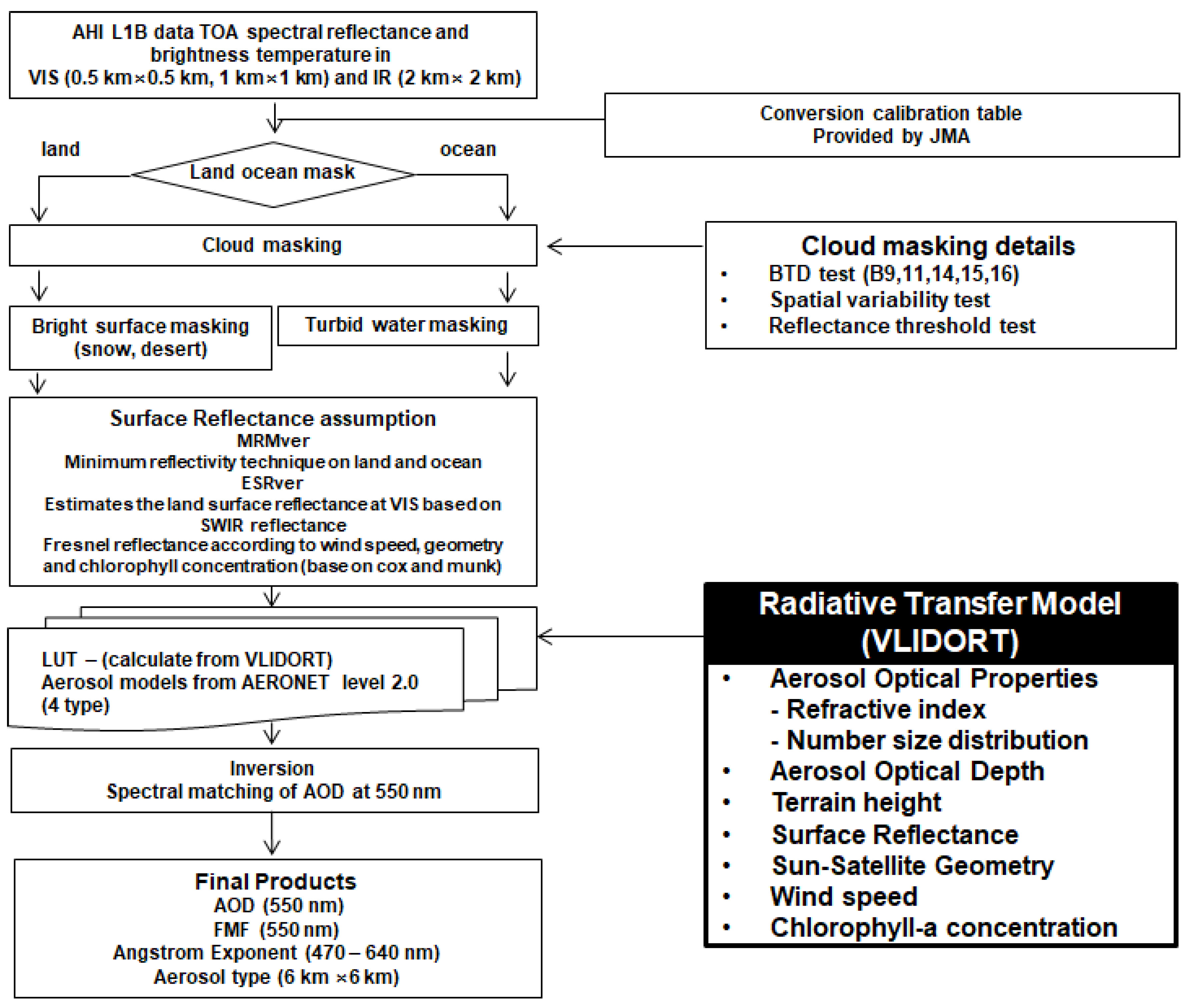
2. Development of the AHI YAER Algorithm

In our previous study, aerosol optical information was retrieved and validated against AERONET for May and June of 2016 using AHI data [27]. Problems remain with surface reflectance (cloud and bright pixel masking) when AOPs are retrieved using measurements at four wavelengths (0.4 to 0.8 µm) regardless of surface type. Therefore, in this study, we used three wavelengths over land, four wavelengths over ocean, and two wavelengths over turbid water area to increase the accuracy of aerosol retrieval. In addition, different threshold values were used for high and low latitudes to mask clouds, and bright pixel making was added newly. Land surface reflectance was estimated from SWIR in addition to existing Minimum Reflectance Method (MRM), and ocean reflectance was from Fresnel equations with the consideration of chlorophyll-a concentration, as discussed in the next section. Here, AOPs were retrieved for February, May, August, and November to represent each season in 2016 using the YAER algorithm [22,23,24], and AOP results were compared with those calculated from AERONET sun-photometer data. The YAER algorithm should be preceded by cloud masking and surface reflectance estimation. In Section 2.1, cloud and bright pixel masking is described. Section 2.2 and Section 2.3 summarize land and ocean surface reflectance estimations. Finally, Section 2.4 presents the inversion method and the flow of the overall YAER algorithm.

2.1. Cloud and Bright-Surface Masking

The AHI YAER algorithm can retrieve aerosol properties only over dark surfaces, so it is important to mask pixels with bright surfaces including desert, snow, and turbid water areas and clouds. The geostationary AHI is equipped with 16 visible and infrared channels, and thus has significantly improved cloud-masking capabilities compared with existing GEO satellites in Asia region. The channel information of AHI is summarized in

Table 1. Specifications for 16 bands of AHI (http://www.data.jma.go.jp/mscweb/en/himawari89/space_segment/spsg_ahi.html).

Band	Center Wavelength (μm)	Spatial Resolution at Sub-Satellite Point (km)
1	0.470	1
2	0.510	1
3	0.640	0.5
4	0.856	1
5	1.61	2
6	2.26	2
7	3.89	2
8	6.24	2
9	6.94	2
10	7.35	2
11	8.56	2
12	9.63	2
13	10.4	2
14	11.2	2
15	12.4	2
16	13.3	2

[28]. In this study, the masking process was applied to upper- and lower-layer clouds, including cirrus, using various brightness temperature differences (BTD) tests. Spatial heterogeneity tests were also performed using the visible channels. In the YAER algorithm, BTD tests using IR channels are first used to detect clouds. The two channels used for BTD calculations differ with layer height. The wavelength dependence of observation sensitivity changes with altitude and can be used to detect upper- and lower-layer clouds [29]. However, AHI does not have a channel at 1.38 μm for cirrus detection. In this study, cirrus clouds are detected using the BTD of band 14 and band 11 instead. The cloud masking process is summarized in

Table 2. Masking tests in the AHI YAER algorithm.

Step	Condition	Classification
1	BTD between Band 15 and Band16 land and ocean: <11 K	high-level cloud over land and ocean
2	BTD between Band 11 and Band 9 land and ocean: <−10 K	low-level cloud over land and ocean
3	BTD between Band 14 and Band 11 land and ocean: <0 K	cirrus cloud over land and ocean
4	BTD between Band 14 max *, Band 14, Band 9 max * and Band 9; Band 14 max * − Band 14 > 15 K; Band 9 max * − Band 9 > 10 K	cloud over land
5	BTD between Band 14 and Band 15 high latitude (segment 1 and 10) ocean: <−1.0 K; mid-low latitude (segment from 2 to 9) ocean: <0.5 K	cloud over ocean
6	STD test at Band 2 and Band 4 > 0.0025	cloud over ocean
7	mean-weighted STD test at Band 1 > 0.0025	cloud over land
8	pseudo GEMI index at Band 3 and Band 4 < 1.87	cloud over land
9	TOA reflectance test at Band 1 > 0.35	cloud over land and ocean
10	NDVI (using Band 3 and Band 4) < −0.01	inland water
11	relationship between Band 6 > 0.2 and NDVISWIR (using Band 5 and Band 6) < 0.05	arid area
12	NDSI (using Band 2 and Band 5) > 0.35 and Band 4 > 0.11	snow and ice over land
13	ratio between Band 4 and Band 5 < 0.82 with Band 6 reflectance > 0.25	cloud over bright land surface
14	difference between Band 3 and linearly-interpolated Band 3 from Band 1 and Band 6 > −0.03	high-turbidity pixels masked over ocean
15	glint angle < 25°	sun glint mask over ocean
16	Constraint in the number of pixels out of 6 × 6 pixels < 3	Step 1–15 for 6 × 6 pixels
17	Band 6 reflectance after aggregation (6 km resolution)	arid area masking

* Maximum BT over past 10 days.

. In step 1, band 15 which is sensitive to water droplets and ice crystals in the upper layer, and band 16 which is affected by CO₂ absorption, were used. If clouds are present at high altitude, bands 15 and 16 have low brightness temperature (BT), but for clouds at low altitude, emission at band 16 is absorbed by CO₂ above thus has lower BT than band 15. This property is used for the high-level cloud masking. In step 2, difference in BT between band 11 and band 9 is used to remove low-level clouds, where band 11 is in atmospheric window region close to band 9. In step 3, band 14 is also in atmospheric window region, and more sensitive to ice crystals than water droplets. Thus, the difference between band 11 and band 14 is used to remove ice clouds in the upper layer. The threshold values for BTD tests are set empirically for respective mission, thus other satellite threshold values must not be adopted directly, due to different calibration and response functions.

Because BT is a parameter sensitive to surface temperature, it is difficult to use a single BT test from geostationary satellites, which have fixed viewing geometries. Therefore, in this study the BTD test was performed by applying the method presented by Kim et al. [21] using the max BT of the pixel for the previous 10 days (step 4). During cloud masking using IR channels (step 5), threshold of −1.0 K is used for segments 1 and 10 of the Himawari Standard Data (HSD) that differ from the threshold of 0.5 K at lower latitudes for segments from 2 to 9 [30]. HSD is provided by Japan Meteorological Agency (JMA) for 10 divided segments from north (#1–#5) to south (#6–#10) [28]. Next, cloud masking using the reflectance of the visible channels is performed. The cloud removal method using the visible channels includes a spatial heterogeneity test, a reflectance threshold test, and a pixel-average constraint. The spatial heterogeneity test is performed during the masking steps 6, 7, and 8. Over ocean, clouds can be masked by a standard deviation (STD) test of reflectance, because the surface is more homogeneous than over land [5,23].

Over land where surface features are inhomogeneous, the problem of mis-detecting clear pixels as cloudy often occurs with a simple STD test. In step 7, we solved this problem by introducing a mean-weighted standard deviation test that accounts for surface inhomogeneity with the threshold value of 0.0025 adopted from previous study [31]. In step 8, a pseudo Global Environment Monitoring Index (GEMI) using bands 3 and 4 was adopted [32,33]. In step 11, desert areas are detected using the NDVI_SWIR and band 6 top-of-atmosphere (TOA) reflectance. In step 12, the Normalized Difference Snow Index (NDSI) is used to detect the degree of snow cover, which is used to mask snow pixels with the reflectance value at band 4 [11]. In step 13, as suggested by Ishida and Nakajima [34], clouds over the desert are masked using the ratio of band 4 to band 5 and threshold test of TOA reflectance at band 6.

In step 14, bright pixels, such as turbid water, are detected based on the work of Li et al. [35], over which the retrieval of aerosol property becomes very difficult with strong contribution of suspending particles. Over clear ocean regions, there is no significant difference between the TOA reflectance of band 3 and that linearly interpolated for band 3 using band 1 and band 6, but large differences appear in turbid water regions where land sediments flow into the water. This is because the sediments have higher reflectance, similar to that of land surfaces. In step 15, Sun-glint zones are calculated from the geometries of solar illumination and satellite viewing and are masked when the glint angle is less than 25°. Each masking test from step 1 to 15 is independent, which masks a pixel if it is classified as cloudy or bright by any of these tests. After aggregating 6 × 6 pixels and going through all bright pixel masking tests from step 1 to 15, if the number of remaining pixels is less than 3 out of 36 pixels, the grid is treated as contaminated thus masked in step 16. Step 17 is a similar test as in step 11 for the aggregated 6x6 pixels.

2.2. Determination of Land Surface Reflectance

Retrieved aerosol properties using visible channels show a dependence on how the surface reflectance is estimated. In this study, two methods are used to retrieve surface reflectance: the MRM, which is used in the MODIS DB C5 algorithm [10] and GOCI-YAER [23,24], and the Estimated Surface Reflectance from SWIR (ESR), which estimates the surface reflectance in the visible range from TOA reflectance at SWIR, as in the MODIS DT [5,6] and MODIS DB C6 [11] algorithms.

2.2.1. Minimum Reflectance Method (MRM)

The surface reflectance using MRM adopts the Lambertian Equivalent Reflectance (LER) calculated using a radiative transfer model, which combines the surface, aerosol, and cloud signals after Rayleigh correction from TOA reflectance using a look-up table (LUT). The calculated LER synthesized for 30 days has a spatial resolution of 1 km (at sub-satellite point), where the lower 6% of the data is averaged to construct the surface reflectance. In determining surface reflectance, lower 6% corresponds to first and second minimum reflectance values in a month to avoid cloud shadow effects in the modified minimum reflectance method [36]. The AHI performs a full-disk observation every 10 min; thus, a database of surface reflectance is constructed at intervals of 10 min. Calculating a representative monthly value from samples at different times indirectly accounts for the Bidirectional Reflectance Distribution Function (BRDF) effect. However, when the monthly surface reflectance database is constructed, discontinuities in surface reflectance across months appear. To minimize the monthly discontinuity, the database was interpolated to daily precision using the average monthly values. In future work, we plan to increase the number of datasets by considering BRDF and estimate surface reflectance with high accuracy [37,38].

2.2.2. SWIR (ESR) Estimates

The DT and DB (C6) algorithms estimate the surface reflectance in the visible region using the 2.1 μm channel of MODIS. According to Levy et al. [6], the NDVI_SWIR (vegetation index using the 1.2 and 2.1 μm channels) can be divided into three categories, and the final surface reflectance estimated using empirical expressions. However, it is difficult to estimate the surface reflectance in urban and agricultural areas. In this study, the aerosol retrieval accuracy was improved by taking the urbanization index into consideration in urban areas [39].

A previous study used another approach to investigate surface reflectance using the 1.6 μm channel of a CAI sensor onboard GOSAT launched by JAXA [40]. They divided the NDVI ranges into 22 subintervals with equal interval of 0.025 and used the relationship between the TOA reflectance at 1.6 μm and the surface reflectance in the visible region for each subinterval. As the NDVI using wavelengths at around 640 nm and 860 nm are affected by aerosols, the NDVI using SWIR bands which is less affected by aerosol is defined as NDVI_SWIR, to calculate the final surface reflectance.

In AHI-YAER algorithm, the data used to calculate the surface reflectance was within 25 km of each measurement site for AERONET Version 2 Level 1.5 AOD 550 nm in East Asia (−5° N–50° N, 110° E–150° E) and the NDVI_SWIR was calculated for each AHI pixel to estimate spectral reflectance information. The AERONET site information is summarized in

Table 3. The site information of AERONET such as geolocation and land type (1 = others; 2 = urban; 3 = cropland. T indicates were used for studying surface reflectance relationships, L^X, O^X indicates were used for validating results over Land and Ocean; X indicates of month information).

Site	Lon.(° E)/Lat.(° N)	Training(Lv1.5)/Validation(Lv2)	Land Type/Average of the Fraction of Land Type within 25 km for Site (%)	Site	Lon.(° E)/Lat.(° N)	Training(Lv1.5) /Validation(Lv2)	Land Type/Average of the Fraction of Land Type within 25 km for Site (%)
Anmyon	126.330/36.539	T/-	1	KORUS_Kyungpook	128.606/35.890	T/L2,5,8	2/13.8
Baengnyeong	124.630/37.966	T/O2,5,8	1	KORUS_Mokpo_NU	126.437/34.913	T/L2,5,8, O2,5,8	3/41.4
Beijing-CAMS	116.317/39.933	T/L2,5,8	2/57.1	KORUS_NIER	126.640/37.569	T/L2,5, O5	1
Beijing	116.381/39.977	T/L2,5	2/57.3	KORUS_Olympic_Park	127.124/37.522	T/L5	2/39.0
Beijing_RADI	116.379/40.005	T/L2	2/55.3	KORUS_Songchon	127.489/37.338	T/L5	3/35.7
Chiayi	120.496/23.496	-/L2	1	KORUS_Taehwa	127.310/37.312	T/L5	1
Chiba_University	140.104/36.625	T/-	1	KORUS_UNIST_Ulsan	129.190/35.582	T/L5,8,11	1
Fukuoka	130.475/33.524	T/L2	2/20.0	Niigata	138.942/37.846	T/-	3/29.2
Ganneung_WNU	128.867/37.771	T/-	1	Noto	137.137/37.334	T/-	1
Gosan_SNU	126.162/33.292	T/L5,8, O5,8	1	Osaka	135.591/34.651	T/L2,5,8,11, O2,5,8,11	1
Gwangju_GIST	126.843/35.228	T/L5	1	Pusan_NU	129.082/35.235	T/L2,5,8,11, O2,5,8,11	2/17.9
Hankuk_UFS	127.266/37.339	-/L2,5,8,11	1	Seoul_SNU	126.951/37.458	T/-	2/55.5
Hokkaido_university	141.341/43.075	T/L2,5,8, O2,5,8	2/13.8	Shirahama	135.357/33.693	T/L2,5, O2,5	1
Hong_Kong_Sheung	114.117/22.483	-/L2,5, O5	1	Ussuriysk	132.163/43.700	T/-	1
KORUS_Baeksa	127.567/37.412	T/L5	3/25.4	XiangHe	116.962/39.754	T/-	3/87.7
KORUS_Daegwallyeong	128.759/37.687	T/L5	1	Yonsei_University	126.935/37.564	T/L2,5,8,11	2/47.5
KORUS_Iksan	127.005/35.962	-/L5	3/60.0

. When AOD is low (AERONET AOD less than 0.1 at 550 nm), aerosol type has no significant effect, and atmospheric (aerosol and Rayleigh) correction was carried out to estimate the surface reflectance at band 3 [41]. The relationship between the collected surface reflectance of band 3(S3) and TOA reflectance of band 5(T5) were analyzed by NDVI_SWIR dividing into interval of 0.01, from 138,744 data of 1 year in 2016. The best linear regression fits were obtained between T5 and S3 for each divided NDVI_SWIR to provide their slope and intercept as a function of NDVI_SWIR:

$${\mathrm{slope}}_{\mathrm{T}5-\mathrm{S}3}=a_1\times {\mathrm{NDVI}}_{\mathrm{SWIR}}+b_1,\mathrm{and}$$

(1)

$${\mathrm{intercept}}_{\mathrm{T}5-\mathrm{S}3}=a_2\times {\mathrm{NDVI}}_{\mathrm{SWIR}}+b_2,$$

(2)

where a₁ (a₂) and b₁ (b₂) are the slope and intercept of the linear regression of the slope_T5-S3 (intercept_T5-S3) with respect to NDVI_SWIR.

The surface reflectance can then be estimated as follows:

$$R_{0.64}^s={\mathrm{slope}}_{\mathrm{T}5-\mathrm{S}3}\times R_{1.6}+{\mathrm{intercept}}_{\mathrm{T}5-\mathrm{S}3},$$

(3)

where $R_{0.64}^s$ represents the surface reflectance to be estimated, and $R_{1.6}$ represents the TOA reflectance of band 5. In the same manner as described above, the surface reflectance at bands 1 and 2 were obtained for atmospheric correction in the dataset collected. From the relationship between the surface reflectance obtained at these wavelengths and that obtained at band 3, a linear empirical equation was constructed. The parameters are summarized in

Table 4. Coefficients for surface reflectance estimates for different surface type in Equations (1) and (2).

	a1	b1	a2	b2
All land types (excluding urban and cropland)	−0.705	0.515	−0.073	0.028
Urbanization fraction 10–30%	−1.605	0.717	−0.008	0.008
Urbanization fraction 30–70%	−1.681	0.812	−0.023	0.003
Urbanization fraction > 70%	−1.944	0.944	−0.021	−0.002
Cropland fraction 10–30%	−1.573	0.807	−0.014	0.001
Cropland fraction 30–70%	−1.096	0.629	−0.047	0.017
Cropland fraction > 70%	−0.592	0.454	−0.065	0.031

and

Table 5. Conversion factor for band 1 (470 nm) and band 2 (510 nm) surface reflectance from band 3 (640 nm) surface reflectance.

	a470	b470	a510	b510
All land types (excluding urban and cropland)	0.561	−0.009	0.661	−0.002
Urbanization fraction 10–30%	0.635	−0.010	0.722	−0.004
Urbanization fraction 30–70%	0.643	−0.013	0.724	−0.004
Urbanization fraction > 70%	0.637	−0.011	0.735	−0.003
Cropland fraction 10–30%	0.645	−0.013	0.736	−0.005
Cropland fraction 30–70%	0.652	−0.015	0.738	−0.006
Cropland fraction > 70%	0.654	−0.006	0.654	−0.006

.

As mentioned above, when estimating the reflectance of the visible region from SWIR, it is possible to estimate more accurate reflectance by considering the urbanization effect. In this study, the percentage fraction of urbanization and cropland were calculated using the MODIS land cover type climate modeling grid product (MCD12C1) [42] and divided into low (10~30%), moderate (30~70%), and high (>70%) respectively. Different empirical formulas to obtain surface reflectance for different surface type are shown in Table 4 and Table 5.

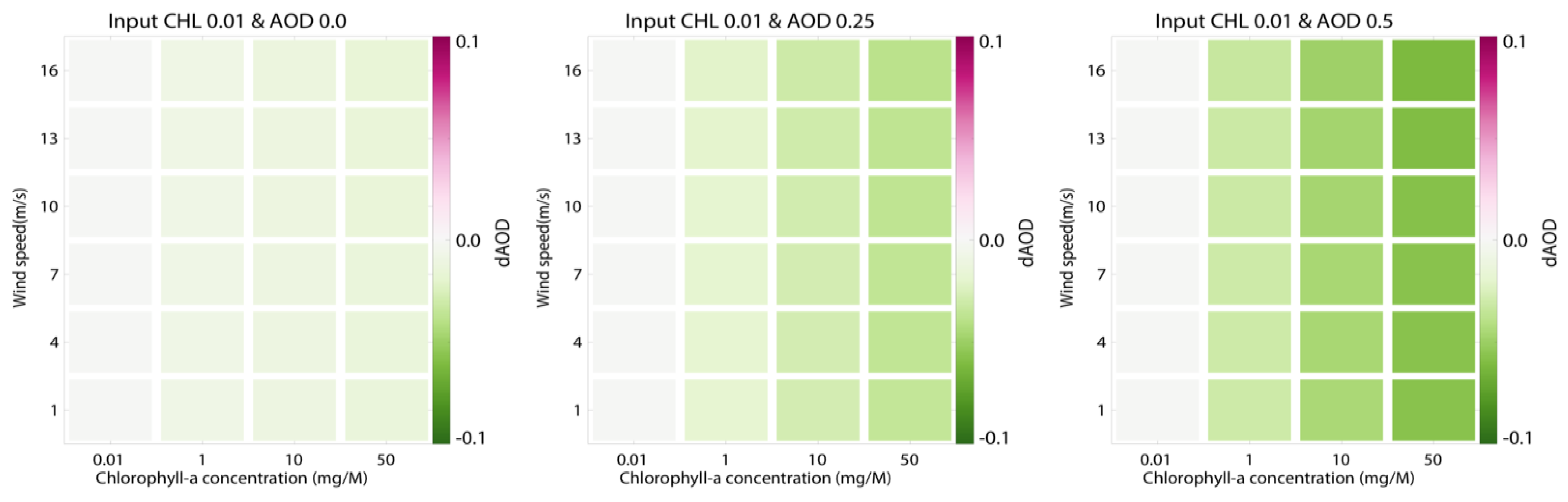
2.3. Determination of Ocean Surface Reflectance

The Fresnel equation is typically used to estimate the ocean surface reflectance according to wind speed [42]. In addition, when the chlorophyll-a concentration is used as an input parameter and the water leaving radiance is considered, this equation can be used in turbid water areas. As reported by Choi et al. [23], the possibility of aerosol retrieval over turbid water areas was confirmed using the MRM. Therefore, in this study the MRM and the Cox and Munk method [43] were used to estimate the ocean surface reflectance.

As in the case of land, a water surface reflectance database is constructed, and the surface reflectance is estimated by interpolating the date to be calculated. However, over turbid water areas, aerosol properties are retrieved using the reflectance of band 1 and band 4, which are relatively less affected by aerosols [24].

Several studies have estimated aerosol properties by evaluating ocean surface reflectance using the Cox and Munk method [8,23,24,41,44]. In this study, ocean surface reflectance is calculated using A Linearized pseudo-spherical Vector Discrete Ordinate Radiative Transfer (VLIDORT) [45] ver. 2.7 considering additional water leaving radiance emitted from the ocean itself. The nodal points of the LUT for estimating the sea-level reflectance were calculated as 1, 4, 7, 10, 13 and 16 ${\mathrm{ms}}^{-1}$ and the chlorophyll-a concentrations as 0.01, 1, 10 and 50 ${\mathrm{mgM}}^{-1}$.

2.4. Inversion Process

The radiative transfer model used to construct the LUT for retrieved aerosol optical properties was VLIDORT ver. 2.7. LUT configurations include surface pressure, sun–satellite geometry and aerosol type. Aerosols are classified into four types: black carbon (BC), mixture (MIX), dust (DU) and non-absorbing (NA), based on AERONET’s FMF and SSA [27,46,47]. Over the ocean, LUTs are constructed considering Fresnel reflectance and ocean BRDF, similar to the land LUT calculations, and are summarized in

Table 6. Look-up table details.

Variable	Value
solar zenith angle (°)	0.01, 10, 20, 30, 40, 50, 60 and 70
viewing zenith angle (°)	0.01, 10, 20, 30, 40, 50, 60 and 70
relative azimuth angle (°)	0.01, 10, 20, 30, 40, 50, 60, 70, … 180
AOD–each reference wavelength	0, 0.25, 0.50, 1.0, 1.5, 2.0 and 3.0
aerosol type	black carbon, non-absorbing, mixture, and dust
surface albedo *	0.0, 0.05, 0.1 and 0.2
terrain height * (km)	0 and 5
band (4)	1 (470 nm), 2 (510 nm), 3 (640 nm) and 4 (860 nm)
wind speed ** (${\mathrm{ms}}^{-1}$)	1, 4, 7, 10, 13 and 16
chlorophyll-a concentration ** (${\mathrm{mgm}}^{-3}$)	0.01, 1, 10 and 50

* only land; ** only ocean.

.

A flowchart of the aerosol retrieval algorithm is shown in Figure 1. The masking method described above was used to screen out pixels with clouds, bright surfaces, and heavily turbid water. Then, inversion was performed with the surface reflectance database using LUTs, pre-calculated using results from a radiative transfer model. When the cloud and bright-surface masking processes were finished as in Table 2, the remaining pixels were collected on a 6 km × 6 km grid (at sub-satellite point), where upper 40% and lower 20% of the 36 pixels were removed. The high and low-reflectance filtering was performed to obtain more reliable data by removing brighter and darker pixels affected by sub pixel cloud and cloud shadows [5,6,23,24].

For the TOA reflectance of each 6 km × 6 km grid (at sub-satellite point), 36 TOA reflectance data points at 1 km (at sub-satellite point) resolution were averaged before masking. We selected the same pixels used for TOA reflectance and averages to create the surface reflectance for each 6 km × 6 km grid. Choosing the same pixels for surface and TOA reflectance reduces error. The external input values required for the aerosol inversion process include chlorophyll-a concentration, wind speed, surface type and terrain height. The wind speed was estimated by interpolating the 6-h reanalysis data on a grid of 0.125° × 0.125° provided by ECMWF, and the chlorophyll-a concentration was interpolated from the data in 1-hour intervals provided by the JAXA [48]. The topographic data of the Global Land One-km Base Elevation Digital Elevation Model (GLOBE) was re-gridded to the AHI grid. MRM version (MRMver) uses the composite method for land and ocean surfaces to estimate the surface reflectance. In ESR version (ESRver), surface reflectance over land was estimated from SWIR, and that over ocean was from the Cox and Munk method with the chlorophyll-a concentration [49]. The AHI has four channels of visible and near infrared bands that are directly used for aerosol retrieval. Band 4 can be used over the dark ocean, but it has a high surface reflectance over land and is not suitable for retrieving aerosol optical properties.

Using the spectral fitting method, the AOD at 550 nm is traced for the given geometry as the input value for each aerosol type using three wavelengths over land and four wavelengths over ocean. Theoretically, all these values should be the same, but in reality they differ because of differences in the calibration corrections of the instrument, errors in the aerosol type construction process, inaccurate surface reflectance estimation, or atmospheric simulation errors in the radiative transfer model. Therefore, the two aerosol types with the smallest standard deviation of AOD at 550 nm were selected, and the final product was obtained considering the weighting function from STD of selected aerosol types. The final product includes AOD, FMF and AE (470–640), and aerosol type at 550 nm at 6-km (at sub-satellite point) resolution. The specific FMF weighting was calculated according to the selected aerosol type. AE was calculated using the AODs at bands 1 and 3.

Later in this work in Section 3 errors are analyzed for the MRMver and ESRver, respectively. In Section 4, products from MRMver and ESRver are merged to improve the accuracy of respective inversion. Different level of merging AHI at surface reflectance and AOD products are considered.

3. Retrieval and Validation Results

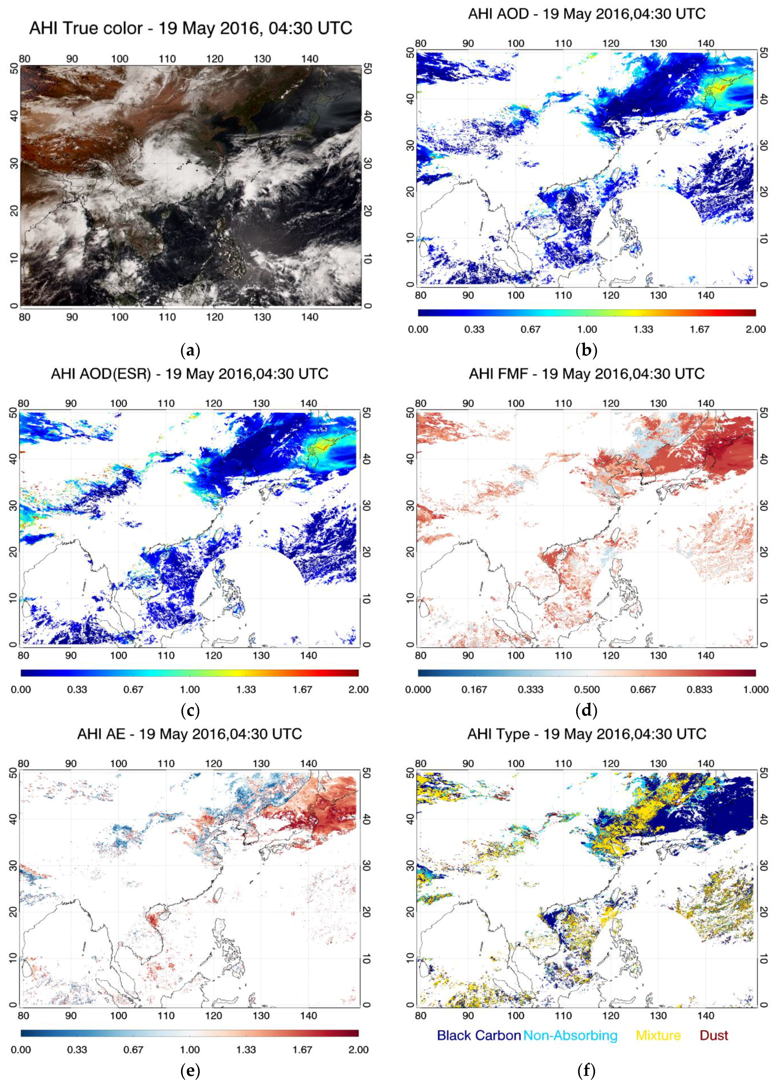
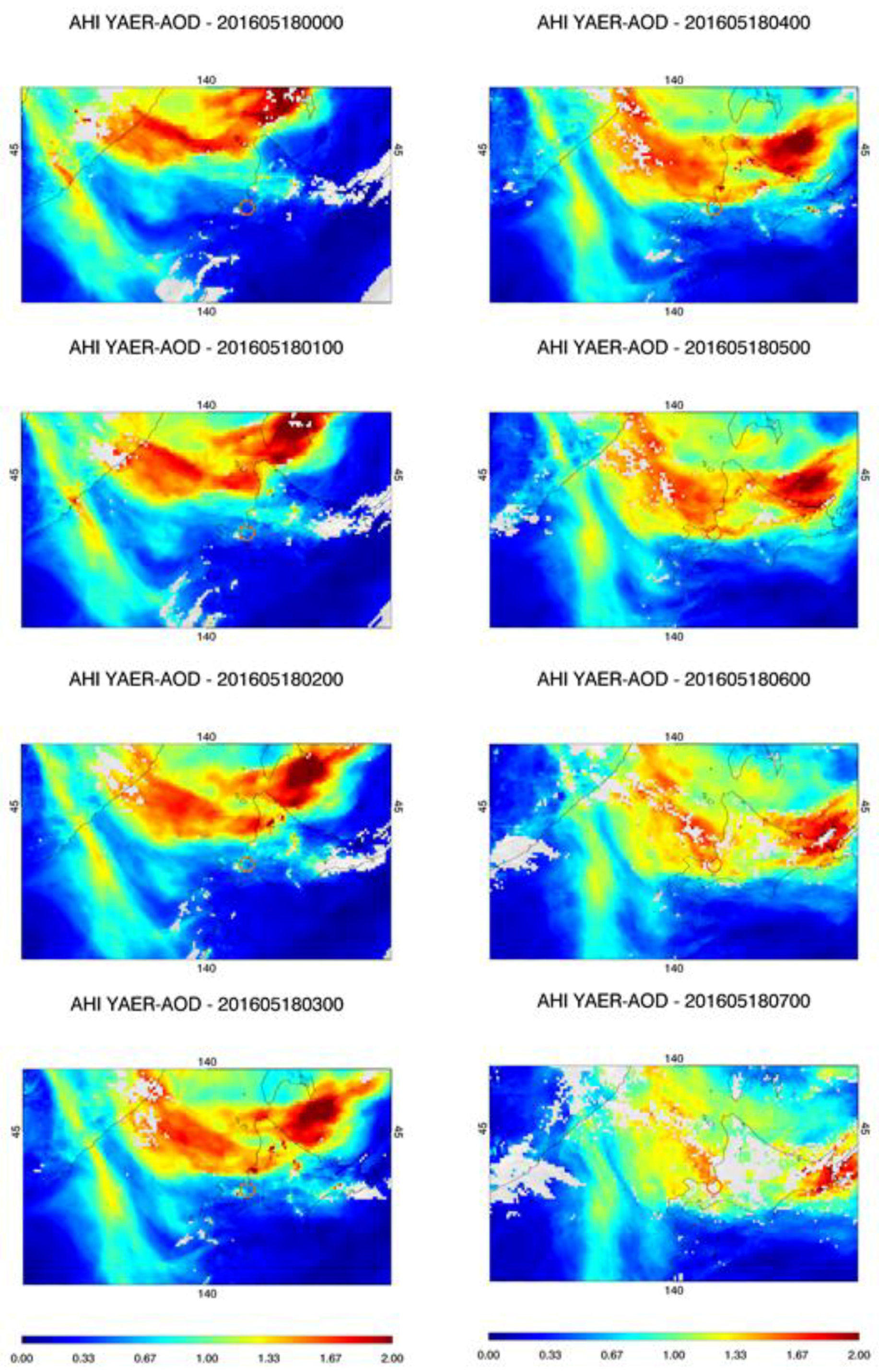
3.1. Retrieval Results from AHI YAER Products

An example of the retrieved aerosol optical properties is shown in Figure 2 for the case of 19 May 2016. Figure 2a is a true color image obtained by AHI, which can visually distinguish clouds, heavy aerosols, and other objects. On this date, an aerosol plume presumed to be smoke passed over the Hokkaido area in Japan. The AOD obtained from (b) MRMver and (c) ESRver is close to 1.5 over this area. Results in this area are consistent despite of using two different methods to estimate the visible surface reflectance. However, ESRver results differ from MRM results in areas where the surface is bright, such as in the western part of China where noisy features are present. The method of estimating surface reflectance using SWIR leads to results that are similar to previous work [50], resulting in errors over bright areas of western China. In Figure 2f, BC aerosol is detected in areas with high AOD, as shown in the true color image in Figure 2a. The FMF shown in Figure 2d is from selected aerosol type, because it is calculated for two selected aerosol types. In contrast, the AE shown in Figure 2e is calculated using the retrieved spectral AOD. Both FMF and AE are related to aerosol size, and thus their values can be inter-compared to some extent in areas where aerosols are present. However, in regions where the aerosol loading is low, the surface signal becomes large and leads to noisy results. In addition, AE is not calculated in many ocean areas. The ocean algorithm generally retrieves AOPs using four wavelengths, but over lightly turbid water areas, only bands 1 and 4 are used, which are less affected by sediments. As there is no spectral AOD in band 3, AE cannot be calculated. In the Pacific Ocean south of Japan, the retrieval is affected by turbid water masking due to the influence of cloud contamination, which makes AE retrieval difficult.

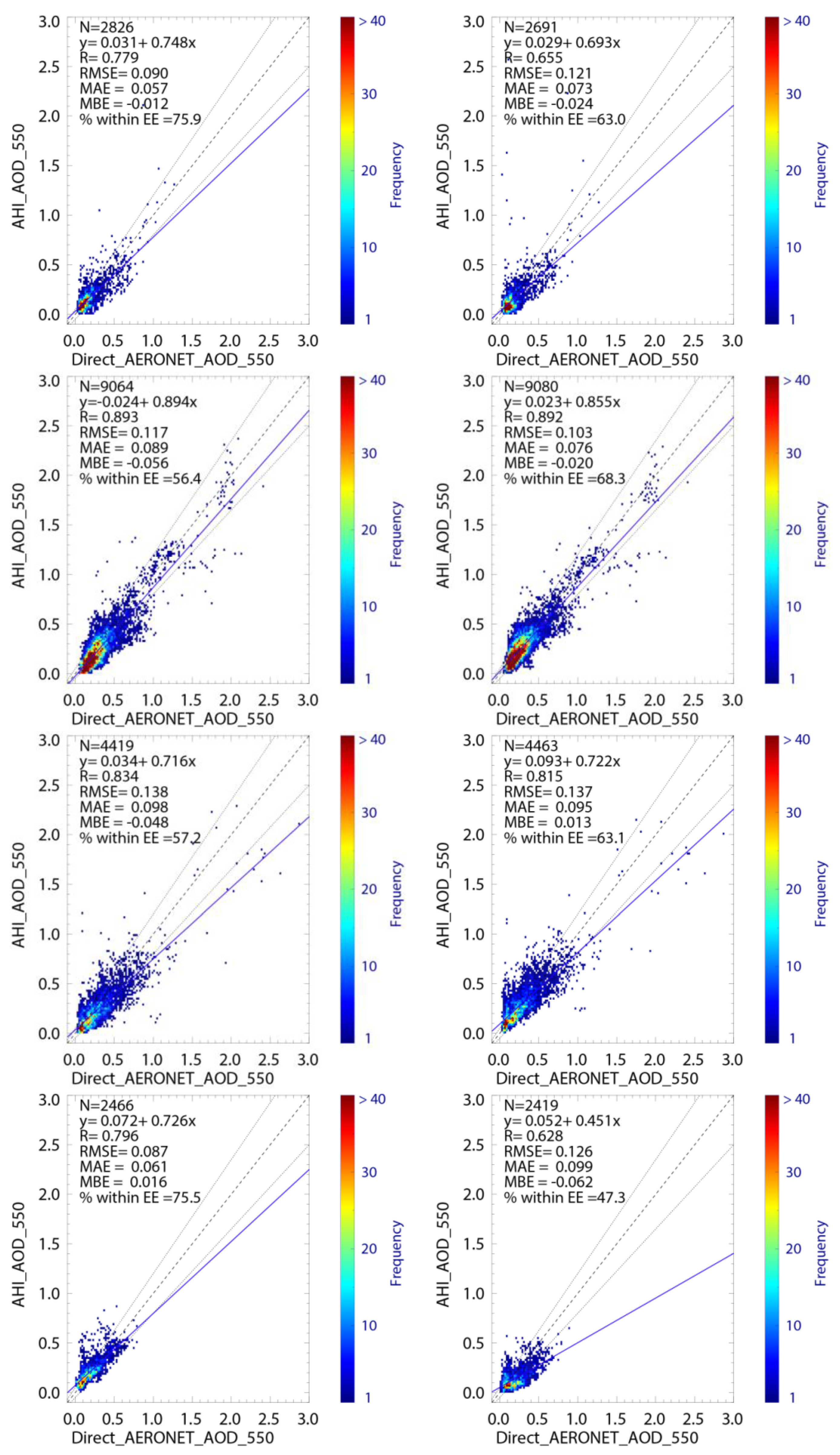
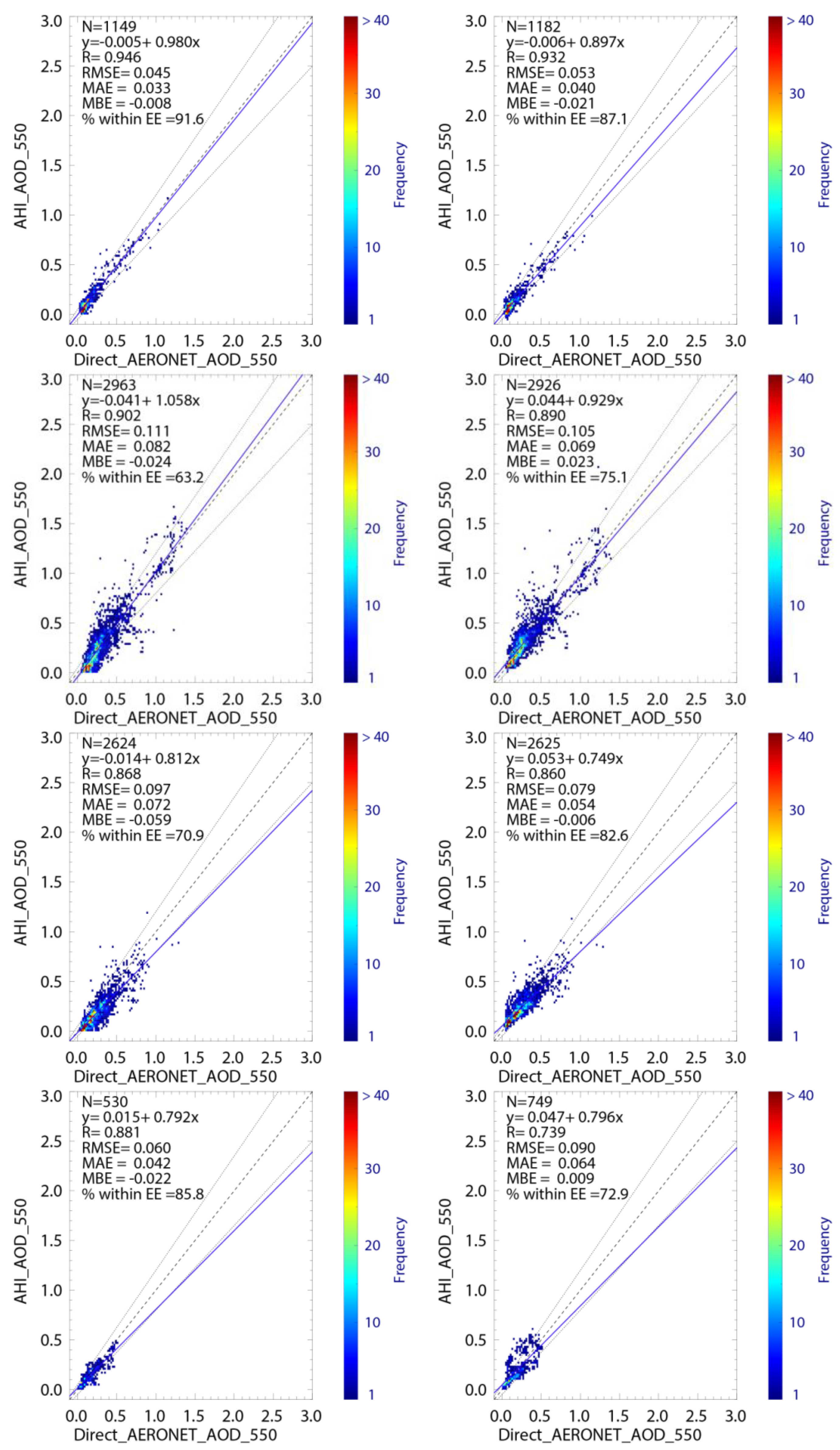
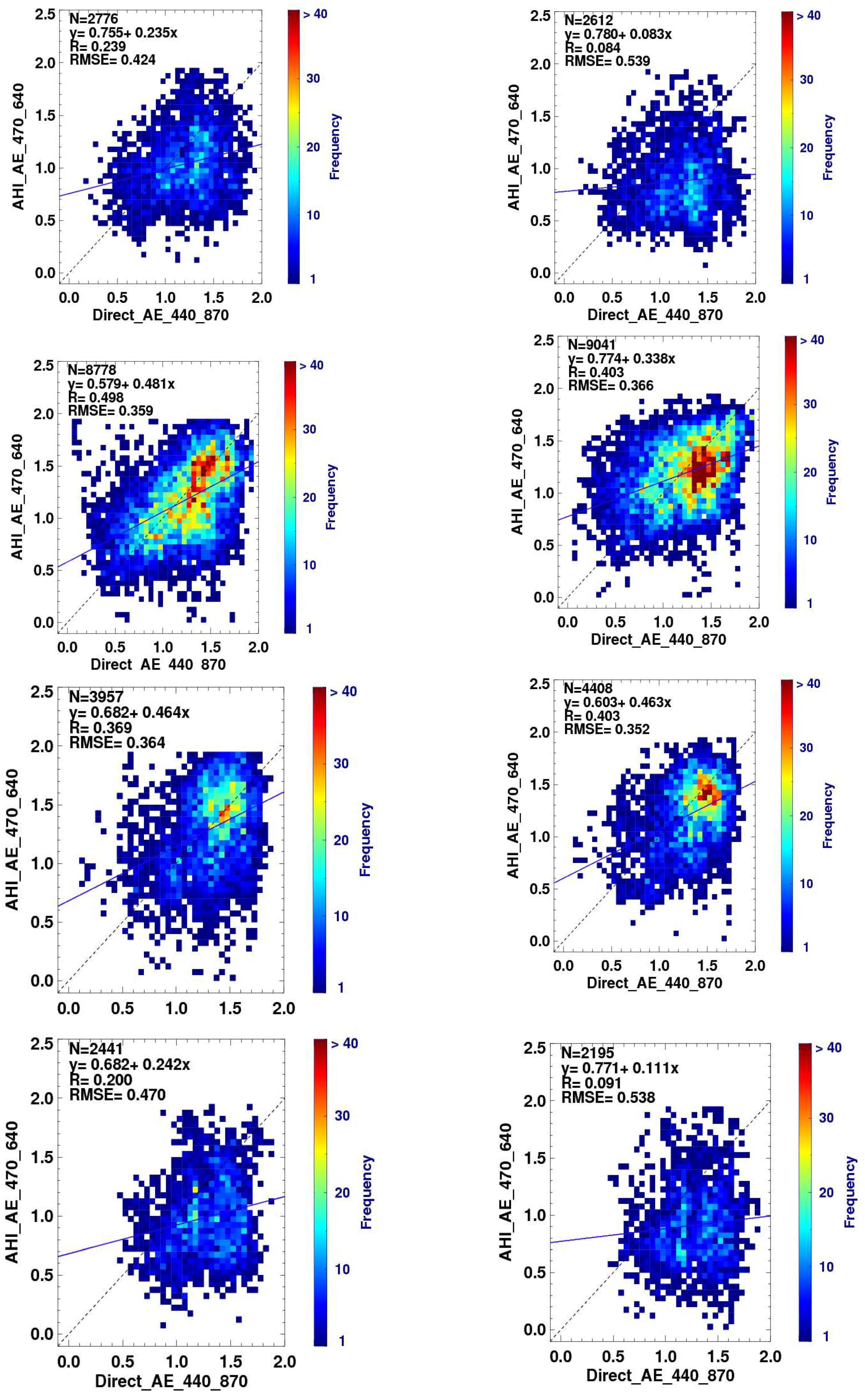
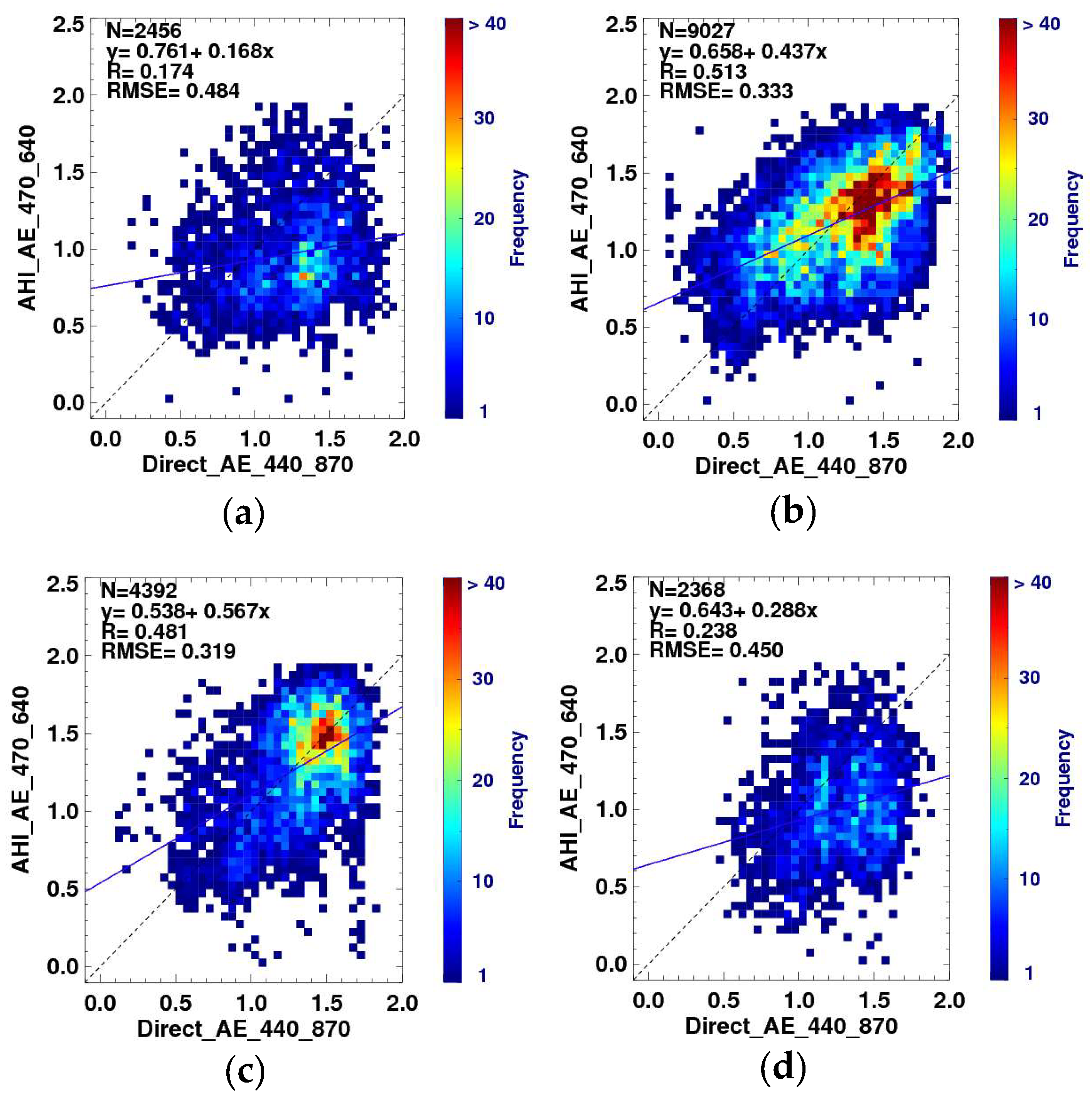
3.2. Validation of AOD and AE

In this section, the performance of two methods of AOP retrieval is validated with the ground-based AERONET sun-photometer network. For spatiotemporal matching, AHI AOD pixels are averaged and compared within 25 km and ±5 min around each AERONET site in the East Asia region (20° N–50° N, 110° E–150° E). Figure 3 shows validation results of MRMver and ESRver AOD over land for each season. Figure 4 shows validation results for the two aerosol product methods over ocean. Validation statistics include linear regression, Pearson correlation coefficient, root mean square error (RMSE), mean absolute error (MAE), median bias error (MBE), and the fraction within the expected error (EE).

First, despite seasonal variations, AOD on land shows reliable results in terms of RMSE, MBE, and EE. Among the validation statistic metrics, EE in particular shows the results to be reasonable. EE for AHI in this study was calculated to compare its retrieval accuracy, based on the EE for MODIS DT products over land [6], i.e., EE = ± 0.05 ± 0.15 × AOD. In the case of MRMver, EE has high values of 75%, 56.4%, 57.2%, and 75.5% for each season. In spring and summer, EE is lower because of surface vegetation changes and cloud contamination, respectively, compared with autumn and winter, but still indicates reliable results. However, ESRver results have EE values of 63.0%, 69.3%, 63.1% 47.3% for each season, with relatively low EE in fall and winter. In East Asia, heavy aerosol loading is estimated in spring and summer, leading to overestimates of surface reflectance by MRMver because of the influence of background AOD (BAOD). In winter, the influence of BAOD is relatively small, and surface reflectance is estimated more accurately by MRMver compared with spring and summer, when estimated AOD has high EE. Surface reflectance estimated by ESRver shows trends opposite to those of MRMver. In spring and summer, with dense vegetation, EE for ESRver has higher values than that for MRMver. It is estimated that ESRver, which uses SWIR, minimizes the effect of BAOD, as SWIR is less sensitive to the presence of aerosol. However, in autumn and winter, vegetation starts to disappear, and the bare surface is exposed. Performances of the two algorithms are shown in

Table 7. Comparison of retrieved AODs from MRM and ESR at selected sites in May 2016.

LAND/Average of a Degree of Urban and Cropland within 25 km for Each Site		N	R	RMSE	MBE	%EE
Beijing (116.381/39.977)/Urban 57.3%	MRM	351	0.979	0.081	−0.017	78.9
	ESR	354	0.969	0.094	−0.016	81.1
Yonsei_university (126.935/37.564)/Urban 47.5%	MRM	552	0.809	0.120	−0.072	45.5
	ESR	552	0.856	0.086	0.033	72.8
KORUS_Iksan (127.005/35.962)/cropland 60.0%	MRM	500	0.900	0.118	−0.042	59.8
	ESR	512	0.905	0.133	0.085	55.7
KORUS_Songchon (127.489/37.338)/cropland 35.7%	MRM	528	0.849	0.161	−0.111	40.2
	ESR	528	0.886	0.121	−0.047	74.6
KORUS_Taehwa (127.310/37.312)/other land type	MRM	514	0.867	0.120	−0.077	49.4
	ESR	524	0.912	0.077	−0.013	86.8
Shirahama (135.357/33.693)/other land type	MRM	183	0.859	0.068	−0.012	77.0
	ESR	181	0.920	0.069	−0.057	64.1

at selected sites for May. The performance of the two algorithms are comparable in terms of R at all sites. However, in terms of %EE, ESR performs better than MRM in general except for Yonsei University, Seoul, Korea and Shirahama, Japan.

Validation results over the ocean are shown in Figure 4. Results over ocean show not only higher EE but also reduced RMSE. Results are better than over land because ocean surface reflectance is darker and more homogeneous than that of land. Unlike MRMver ocean products, ESRver ocean products use chlorophyll-a concentrations as an input. However, the chlorophyll-a concentration data from JAXA used in this study are only available since March 2016, thus, no chlorophyll-a concentration data for February. For February, we performed sensitivity tests of AOD, with respect to errors in chlorophyll-a concentrations. Figure 5 shows the difference between AOD retrieved by imposing errors in chlorophyll-a concentration (1, 10, 50) to the simulated visible reflectance by the forward model (chlorophyll-a = 0.01, AOD = 0, 0.25, 0.5) which is known true condition. As shown in Figure 5, the AOD error from errors in chlorophyll-a concentrations was less than 0.08. Considering that the average chlorophyll-a concentration in East Asia is 0.02 mg/M, the effect on final AOD is expected to be small. Because the peak chlorophyll-a concentration does not appear in February, a value of 0.02 mg/M, which is the East Asian average, was assumed [51].

Validation results for AE are shown in Figure 6. This figure shows that MRMver AE are closer to a one-to-one line compared to ESRver AE. Also, RMSE and the correlation coefficient are similar or higher accuracy than ESRver AE. MRMver AE results are slightly higher than ESRver AE in general. This explains the difference between the spectral AOD calculated at each wavelength. The composite method can reflect spectral changes well, whereas the results of ESRver using NDVI_SWIR and TOA reflectance at band 5 are similar to calculating the reflectance at each wavelength with empirical formulas. This does not reflect spectral changes better than the composite method.

However, in May and August, when aerosol loading is high in northeast Asia, the results are similar because the aerosol signal is more sensitive to spectral AOD, thus in higher accuracy. However, the retrieved AE differs between the two methods in February and November when the aerosol load is relatively low.

3.3. Error Analysis

Aerosol optical information generated by satellite remote sensing has various error sources, including errors in surface reflectance estimates, cloud contamination, and aerosol type assumptions. In this section, we compare the AOD of AHI with that of AERONET to analyze the error quantitatively.

3.3.1. Analysis of Two Land Products

In Figure 7, the medians of the difference between the two products of AHI AOD retrieval and AERONET AOD are plotted with respect to NDVI and surface reflectance over land, and AERONET AOD and AERONET AE over ocean. The red and green colors indicate that the AHI AOD is underestimated and overestimated, respectively, and the number of data points in each bin is also shown. As shown in Figure 7a for the MRMver, the AOD error according to the NDVI is close to zero. However, results in May, when AOD is large in East Asia, show an overall negative bias regardless of NDVI. In May, MRMver is affected by BAOD, which leads to overestimates of surface reflectance. However, with monsoon rains in East Asia from July to August, there are higher probabilities to find clear pixels with low BAOD in the atmosphere, which permits more accurate surface reflectance estimates. AOD in August was estimated using the linearly interpolated surface reflectance data of July, August, and September. The assumption that vegetation changes linearly over the search window period may result in errors. Figure 7c shows the error analysis for ESRver, which indicates high accuracy in May and August when vegetation is relatively dense. Unlike MRMver, more accurate ESRver AOD was retrieved, because ESRver is less affected by BAOD. However, in February and November, when vegetation decays to directly expose the surface, estimates from SWIR are less accurate, resulting in larger biases than for MRMver.

Figure 7b,d present an analysis of the surface reflectance of band 1 estimated using the two retrieval methods, MRMver and ESRver. The analysis was performed using only data with AERONET AOD less than 0.2 to analyze errors in the surface reflectance signal. MRMver and ESRver both showed accurate results. However, in the case of MRMver, the error is large for the last surface reflectance bin of the month. Although this may result from the small number of validation points, it could also be attributed to a limitation of the MRMver method, which shows the same tendency for all four months.

3.3.2. Analysis of Two Ocean Products

Figure 8 shows results for the ocean products, analyzing the difference between the two AHI retrieval methods and AERONET AOD as a function of AERONET AOD and AE. The difference with respect to AERONET AOD shows a relatively large error for large AOD bins in August, which can be attributed to the small number of validation points, as described above.

The ESRver results in Figure 8c,d show that AHI AOD has a positive bias, including for lower AE bins in November. It is presumed that this results from the influence of turbid water near coastal regions. As shown in Figure 8a,b, MRMver shows reasonable results over turbid water areas with signals similar to those over land. Furthermore, it uses bands 1 and 4, which are less affected by the reflectance of turbid water. In contrast, ESRver uses bands 1 and 4, which are not influenced by chlorophyll, but the retrieved AOD shows a positive bias. The chlorophyll-a concentration was considered only when simulating the water-leaving radiance over turbid water areas. In actual turbid water areas, there are various suspended substances such as Colored Dissolved Organic Matter (CDOM).

The two methods’ estimations of AOD over land have opposite trends in accuracy. Thus, the two merged AOD products show higher accuracy. One merging approach is to merge AOD between the MRMver and the ESRver, and another is to re-retrieve AOD using the merged surface reflectance from the MRMver and ESRver methods.

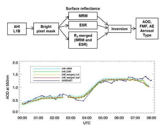
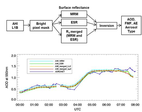
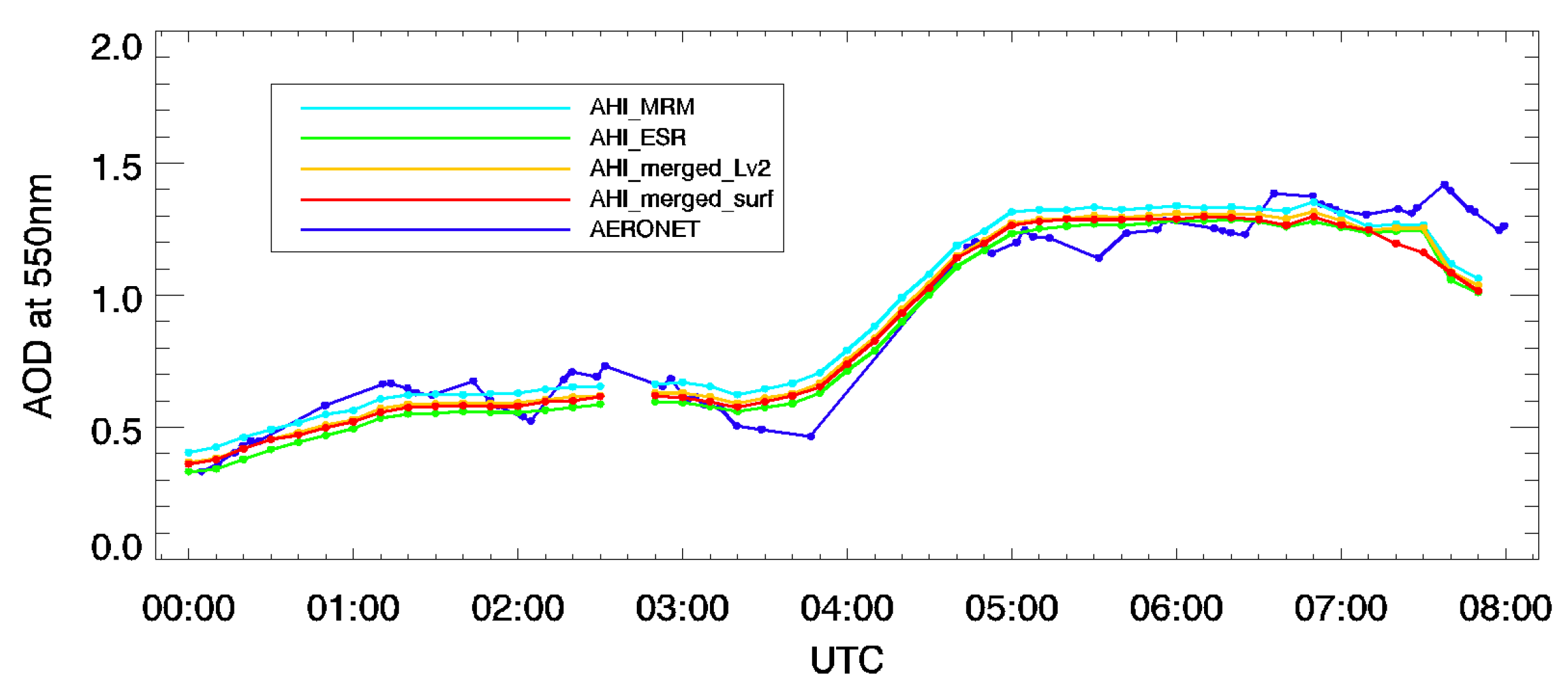
4. AHI YAER Merged Aerosol Products

The method of estimating land surface reflectance using the above-mentioned merging of MRM and ESR estimates is similar to the method used for the MODIS DT and DB algorithms. The DT algorithm has high accuracy over vegetated areas, and the DB algorithm has high accuracy over bright surfaces, such as urban and cropland areas. The two products are merged using the NDVI for quality assurance (QA) and result in a more accurate AOD product. Similarly, in this study we merged the AOD retrieved by the MRMver and ESRver methods for a higher accuracy product.

The MODIS merged product uses the DB AOD for NDVI < 0.2, the average value if QA is the same at 0.2 ≤ NDVI < 0.3, and the DT AOD at NDVI ≥ 0.3. Bilal et al. [52] discussed results from the MODIS merged product. According to previous studies [8,53], although the method of merging according to NDVI is of high quality, the average of the DT and DB AODs for all retrieved pixels shows similar or higher accuracy than the NDVI-based merge. Therefore, in this study we estimate the optimal AOD by taking the average of two methods’ AOD, which is labeled the L2 merged product. As mentioned in Section 3, the results from ESR show higher accuracy in May and August, when the vegetation is dense, and MRM shows higher accuracy in February and November when vegetation is sparse. A more reliable surface reflectance can be obtained by averaging the surface reflectance estimated from the two methods. This improvement likely results from a moderating of the weaknesses of the surface reflectance estimated by each method. The AOD retrieved from the merged surface reflectance is called the Rs merged product, and the results of a validation with AERONET data is shown in

Table 8. Validation results for the Rs merged product, L2 merged product and AERONET AOD. Bold font indicates a higher validation score than that of MRMver and ESRver.

Rs Merged/L2 Merged	N	R	RMSE	MBE	%EE
February	2624/2624	0.727/0.776	0.107/0.087	0.007/−0.012	78.2/83.2
May	9086/9064	0.905/0.906	0.096/0.103	0.01/−0.039	76.3/68.3
August	4468/4419	0.840/0.838	0.131/0.129	0.03/−0.017	65.2/63.7
November	2486/2466	0.809/0.78	0.086/0.089	−0.011/−0.016	75.9/71.2

, along with a similar validation for the L2 merged product.

Results for the L2 merged product for February, May and August are similar to or better than the respective unmerged results in terms of R, RMSE, MBE, and %EE. In November, the ESRver product is of lower quality than that from MRMver in terms of EE, however this EE still has a reasonably high value of 71.2%. Results for the R_s merged product indicate higher accuracy than unmerged results for all seasons from February to November, suggesting that the surface reflectance at each wavelength is estimated reliably. As shown in Figure 9, the AE for the merged results are close to a one-to-one line compared with AERONET data overall, and the correlation coefficient reaches a maximum of 0.513. The correlation coefficient of AE is not high compared to that of AOD, but this is a difficult retrieval, as noted in previous studies [7].

The AHI makes full-disk observations every 10 min, and the results of the diurnal variation in the four retrieved AODs are shown in Figure 10 together with the observed AERONET data. A noticeable aerosol plume passed over the Hokkaido area on 18 May 2016 is shown Figure 11. As LEO satellite passes over certain region at only specific local time, it cannot monitor aerosol’s daily fluctuation. As shown in Figure 10 and Figure 11, GEO satellite can monitor various events such as a sudden increase and decrease in aerosol loading. Results from the four AODs are in line with the observed AERONET AOD. However, AHI AOD accuracy decreases after 0700 UTC, possibly due to the increased solar zenith angle and the bright pixel masking issue. In addition, in the morning MRM seems to be slightly more accurate, but in the afternoon ESRver is closer to the AERONET values. This suggests that the merged product may be improved by changing the weightings, which need to be investigated further in future work. The AHI results shown here are smooth, as we used average values for the area within a 25 km radius around each AERONET site. There are noticeable differences in AOD for 0330-0400 UTC, during which the heavy aerosol plume passed across Hokkaido, with its center passing just north of Hokkaido University AERONET site. As the retrieved products from AHI are for area within 25 km radius of the site, they tend to overestimate the AERONET values.

5. Conclusions

The AHI has multiple infrared channels, which are useful in masking features that affect aerosol retrieval. In addition, multiple visible and near-infrared channels provide a great advantage in aerosol property retrieval from GEO. Therefore, in this study we retrieved and validated AOPs using multiple channels based on the surface reflectance calculated by two methods over land, both of which showed reliable results. The error characteristics of each product were presented, along with those of the L2 merged product.

Moreover, by merging the estimated surface reflectance, more stable surface reflectance can be obtained, as shown by results from the R_s merged product. Merged products using the retrieved AODs may not show improved results in terms of lower EE than the AOD produced by each respective method. However, stable surface reflectance is obtained from the R_s merged product, which can be explained by the improved accuracy of the calculated AE.

Results over ocean were compared using the MRM method and the Cox and Munk method with consideration of chlorophyll-a concentrations. Areas of heavily turbid water were removed using the water surface reflectance increases at about 600 nm, as in previous work, but aerosol properties were still retrieved over light turbid water areas. Band 4 is relatively unaffected by turbid water, but band 1 reflectance is somewhat affected, resulting in an underestimate of AOD. However, results from ESRver show the opposite trend as those from MRMver. Because chlorophyll-a concentrations are only considered when explaining the water leaving radiance in turbid water areas where aerosol properties are retrieved, the water surface reflectance is underestimated, leading to an overestimate of AOD.

Next-generation geostationary satellites have a high temporal resolution in addition to high spatial resolution. Thus, their contribution to accurate retrieval of AOPs is significant for studies on aerosol transport in Asia. Retrieved AOD on a 10-min interval by AHI has a similar pattern to that of AERONET, and results from each merged product have more accurate results than each non-merged product. Cloud masking is also important for accurate AOP results. The AHI, a next-generation GEO satellite, shows significantly improved AOD retrieval capabilities compared with past-generation meteorological satellites, such as the MI, MTSAT, and GOES. Despite the reduced number of channels in the visible and NIR of AHI compared with GOCI, AOP products from AHI have accuracies comparable to GOCI. Synergistic products between AHI, GOCI, the next-generation GOCI-2, and the Geostationary Environmental Monitoring Spectrometer (GEMS) on board the GEOKOMPSAT-2B mission will improve the accuracy of AOP from GEO and expand its data coverage. The algorithms presented in this study are directly applicable to the Himawari-9 satellites equipped with the same sensors as the Himawari-8 and the Advanced Meteorological Imager (AMI) on board the GEOKOMPSAT-2A to be launched in 2018, with some modifications.

References

1. Lau, K.M.; Kim, K.M. Observational relationships between aerosol and Asian monsoon rainfall, and circulation. Geophys. Res. Lett. 2006, 33. [Google Scholar] [CrossRef]
2. Stocker, T.F.; Qin, D.; Plattner, G.-K.; Tignor, M.M.; Allen, S.K.; Boschung, J.; Nauels, A.; Xia, Y.; Bex, V.; Midgley, P.M. Climate Change 2013: The Physical Science Basis. Contribution of Working Group I to the Fifth Assessment Report of IPCC the Intergovernmental Panel on Climate Change; Cambridge University Press: Cambridge, UK, 2014. [Google Scholar]
3. Harrison, R.M.; Yin, J. Particulate matter in the atmosphere: Which particle properties are important for its effects on health? Sci. Total Environ. 2000, 249, 85–101. [Google Scholar] [CrossRef]
4. Lim, S.S.; Vos, T.; Flaxman, A.D.; Danaei, G.; Shibuya, K.; Adair-Rohani, H.; AlMazroa, M.A.; Amann, M.; Anderson, H.R.; Andrews, K.G.; et al. A comparative risk assessment of burden of disease and injury attributable to 67 risk factors and risk factor clusters in 21 regions, 1990–2010: A systematic analysis for the global burden of disease study 2010. Lancet 2012, 380, 2224–2260. [Google Scholar] [CrossRef]
5. Remer, L.A.; Kaufman, Y.; Tanré, D.; Mattoo, S.; Chu, D.; Martins, J.V.; Li, R.-R.; Ichoku, C.; Levy, R.; Kleidman, R. The MODIS aerosol algorithm, products, and validation. J. Atmos. Sci. 2005, 62, 947–973. [Google Scholar] [CrossRef]
6. Levy, R.C.; Remer, L.A.; Mattoo, S.; Vermote, E.F.; Kaufman, Y.J. Second-generation operational algorithm: Retrieval of aerosol properties over land from inversion of Moderate Resolution Imaging Spectroradiometer spectral reflectance. J. Geophys. Res. 2007, 112, D13211. [Google Scholar] [CrossRef]
7. Levy, R.C.; Remer, L.A.; Kleidman, R.G.; Mattoo, S.; Ichoku, C.; Kahn, R.; Eck, T.F. Global evaluation of the collection 5 MODIS dark-target aerosol products over land. Atmos. Chem. Phys. 2010, 10, 10399–10420. [Google Scholar] [CrossRef] [Green Version]
8. Levy, R.; Mattoo, S.; Munchak, L.; Remer, L.; Sayer, A.; Hsu, N. The collection 6 MODIS aerosol products over land and ocean. Atmos. Meas. Tech. 2013, 6, 159–259. [Google Scholar] [CrossRef]
9. Hsu, N.C.; Tsay, S.-C.; King, M.D.; Herman, J.R. Aerosol properties over bright-reflecting source regions. IEEE Trans. Geosci. Remote Sens. 2004, 42, 557–569. [Google Scholar] [CrossRef]
10. Hsu, N.C.; Tsay, S.-C.; King, M.D.; Herman, J.R. Deep blue retrievals of Asian aerosol properties during Ace-Asia. IEEE Trans. Geosci. Remote Sens. 2006, 44, 3180–3195. [Google Scholar] [CrossRef]
11. Hsu, N.C.; Jeong, M.J.; Bettenhausen, C.; Sayer, A.M.; Hansell, R.; Seftor, C.S.; Huang, J.; Tsay, S.C. Enhanced Deep Blue aerosol retrieval algorithm: The second generation. J. Geophys. Res. 2013, 118, 9296–9315. [Google Scholar] [CrossRef]
12. Kalashnikova, O.V.; Garay, M.J.; Martonchik, J.V.; Diner, D.J. MISR Dark Water aerosol retrievals: Operational algorithm sensitivity to particle non-sphericity. Atmos. Meas. Tech. 2013, 6, 2131–2154. [Google Scholar] [CrossRef]
13. Martonchik, J.V.; Kahn, R.A.; Diner, D.J. Retrieval of aerosol properties over land using MISR observations. In Satellite Aerosol Remote Sensing Over Land; Springer: Berlin/Heidelberg, Germany, 2009; pp. 267–293. [Google Scholar]
14. Garay, M.J.; Kalashnikova, O.V.; Bull, M.A. Development and assessment of a higher-spatial-resolution (4.4  km) MISR aerosol optical depth product using AERONET-DRAGON data. Atmos. Chem. Phys. 2017, 17, 5095–5106. [Google Scholar] [CrossRef]
15. Dubovik, O.; Herman, M.; Holdak, A.; Lapyonok, T.; Tanré, D.; Deuzé, J.L.; Ducos, F.; Sinyuk, A.; Lopatin, A. Statistically optimized inversion algorithm for enhanced retrieval of aerosol properties from spectral multi-angle polarimetric satellite observations. Atmos. Meas. Tech. 2011, 4, 975–1018. [Google Scholar] [CrossRef] [Green Version]
16. Kim, J.; Yoon, J.M.; Ahn, M.; Sohn, B.; Lim, H. Retrieving aerosol optical depth using visible and mid-IR channels from geostationary satellite MTSAT-1R. Int. J. Remote Sens. 2008, 29, 6181–6192. [Google Scholar] [CrossRef]
17. Yoon, J.M.; Kim, J.; Lee, J.H.; Cho, H.K.; Sohn, B.-J.; Ahn, M.-H. Retrieval of aerosol optical depth over East Asia from a geostationary satellite, MTSAT-1R. Asia Pac. J. Atmos. Sci. 2007, 43, 49–58. [Google Scholar]
18. Bernard, E.; Moulin, C.; Ramon, D.; Jolivet, D.; Riedi, J.; Nicolas, J.M. Description and validation of an AOT product over land at the 0.6 μm channel of the SEVIRI sensor onboard MSG. Atmos. Meas. Tech. 2011, 4, 2543–2565. [Google Scholar] [CrossRef] [Green Version]
19. Knapp, K.; Frouin, R.; Kondragunta, S.; Prados, A. Toward aerosol optical depth retrievals over land from GOES visible radiances: Determining surface reflectance. Int. J. Remote Sens. 2005, 26, 4097–4116. [Google Scholar] [CrossRef]
20. Wang, J. Geostationary satellite retrievals of aerosol optical thickness during Ace-Asia. J. Geophys. Res. 2003, 108. [Google Scholar] [CrossRef]
21. Kim, M.; Kim, J.; Wong, M.S.; Yoon, J.; Lee, J.; Wu, D.; Chan, P.; Nichol, J.E.; Chung, C.-Y.; Ou, M.-L. Improvement of aerosol optical depth retrieval over Hong Kong from a geostationary meteorological satellite using critical reflectance with background optical depth correction. Remote Sens. Environ. 2014, 142, 176–187. [Google Scholar] [CrossRef]
22. Kim, M.; Kim, J.; Jeong, U.; Kim, W.; Hong, H.; Holben, B.; Eck, T.F.; Lim, J.H.; Song, C.K.; Lee, S.; et al. Aerosol optical properties derived from the DRAGON-NE Asia campaign, and implications for a single-channel algorithm to retrieve aerosol optical depth in spring from Meteorological Imager (MI) on-board the Communication, Ocean, and Meteorological Satellite (COMS). Atmos. Chem. Phys. 2016, 16, 1789–1808. [Google Scholar]
23. Choi, M.; Kim, J.; Lee, J.; Kim, M.; Park, Y.-J.; Jeong, U.; Kim, W.; Hong, H.; Holben, B.; Eck, T.F.; et al. GOCI Yonsei Aerosol Retrieval (YAER) algorithm and validation during the DRAGON-NE Asia 2012 campaign. Atmos. Meas. Tech. 2016, 9, 1377–1398. [Google Scholar] [CrossRef]
24. Choi, M.; Kim, J.; Lee, J.; Kim, M.; Park, Y.-J.; Holben, B.; Eck, T.F.; Li, Z.; Song, C.H. GOCI Yonsei aerosol retrieval version 2 products: An improved algorithm and error analysis with uncertainty estimation from 5-year validation over East Asia. Atmos. Meas. Tech. 2018, 11, 385–408. [Google Scholar] [CrossRef]
25. Schmit, T.J.; Gunshor, M.M.; Menzel, W.P.; Gurka, J.J.; Li, J.; Bachmeier, A.S. Introducing the next-generation Advanced baseline imager on GOES-R. Bull. Am. Meteorol. Soc. 2005, 86, 1079–1096. [Google Scholar] [CrossRef]
26. Kikuchi, M.; Murakami, H.; Suzuki, K.; Nagao, T.M.; Higurashi, A. Improved Hourly Estimates of Aerosol Optical Thickness Using Spatiotemporal Variability Derived From Himawari-8 Geostationary Satellite. IEEE Trans. Geosci. Remote Sens. 2018, 1–14. [Google Scholar] [CrossRef]
27. Lim, H.; Choi, M.; Kim, M.; Kim, J.; Chan, P.W. Retrieval and validation of aerosol optical properties using Japanese next generation meteorological satellite, Himawari-8. Korean J. Remote Sens. 2016, 32, 681–691. [Google Scholar] [CrossRef]
28. Bessho, K.; Date, K.; Hayashi, M.; Ikeda, A.; Imai, T.; Inoue, H.; Kumagai, Y.; Miyakawa, T.; Murata, H.; Ohno, T.; et al. An introduction to Himawari-8/9—Japan’s New-generation Geostationary Meteorological Satellites. J. Meteorol. Soc. Jpn. 2016, 94, 151–183. [Google Scholar] [CrossRef]
29. Iwabuchi, H.; Saito, M.; Tokoro, Y.; Putri, N.S.; Sekiguchi, M. Retrieval of radiative and microphysical properties of clouds from multispectral infrared measurements. Prog. Earth Planet. Sci. 2016, 3, 32. [Google Scholar] [CrossRef]
30. Frey, R.A.; Ackerman, S.A.; Liu, Y.; Strabala, K.I.; Zhang, H.; Key, J.R.; Wang, X. Cloud Detection with MODIS. Part I: Improvements in the MODIS Cloud Mask for Collection 5. J. Atmos. Ocean. Technol. 2008, 25, 1057–1072. [Google Scholar] [CrossRef]
31. Wang, Y.; Chen, L.; Li, S.; Wang, X.; Yu, C.; Si, Y.; Zhang, Z. Interference of heavy aerosol loading on the VIIRS Aerosol Optical Depth (AOD) Retrieval Algorithm. Remote Sens. 2017, 9, 397. [Google Scholar] [CrossRef]
32. Pinty, B.; Verstraete, M. GEMI: A non-linear index to monitor global vegetation from satellites. Plant Ecol. 1992, 101, 15–20. [Google Scholar] [CrossRef]
33. Kopp, T.J.; Thomas, W.; Heidinger, A.K.; Botambekov, D.; Frey, R.A.; Hutchison, K.D.; Iisager, B.D.; Brueske, K.; Reed, B. The VIIRS Cloud Mask: Progress in the first year of S-NPP toward a common cloud detection scheme. J. Geophys. Res. 2014, 119, 2441–2456. [Google Scholar] [CrossRef]
34. Ishida, H.; Nakajima, T.Y. Development of an unbiased cloud detection algorithm for a Spaceborne multispectral imager. J. Geophys. Res. Atmos. 2009, 114. [Google Scholar] [CrossRef]
35. Rong-Rong, L.; Kaufman, Y.J.; Bo-Cai, G.; Davis, C.O. Remote sensing of suspended sediments and shallow coastal waters. IEEE Trans. Geosci. Remote Sens. 2003, 41, 559–566. [Google Scholar] [CrossRef]
36. Fukuda, S.; Nakajima, T.; Takenaka, H.; Higurashi, A.; Kikuchi, N.; Nakajima, T.Y.; Ishida, H. New approaches to removing cloud shadows and evaluating the 380 nm surface reflectance for improved aerosol optical thickness retrievals from the GOSAT/TANSO-Cloud and Aerosol Imager. J. Geophys. Res. 2013, 118. [Google Scholar] [CrossRef]
37. Wang, Y.; Lyapustin, A.I.; Privette, J.L.; Morisette, J.T.; Holben, B. Atmospheric correction at AERONET locations: A new science and validation data set. IEEE Trans. Geosci. Remote Sens. 2009, 47, 2450–2466. [Google Scholar] [CrossRef]
38. Lyapustin, A.; Wang, Y.; Laszlo, I.; Kahn, R.; Korkin, S.; Remer, L.; Levy, R.; Reid, J.S. Multiangle implementation of atmospheric correction (MAIAC): 2. Aerosol algorithm. J. Geophys. Res. 2011, 116, D03211. [Google Scholar] [CrossRef]
39. Gupta, P.; Levy, R.C.; Mattoo, S.; Remer, L.A.; Munchak, L.A. A surface reflectance scheme for retrieving aerosol optical depth over urban surfaces in MODIS Dark Target retrieval algorithm. Atmos. Meas. Tech. 2016, 9, 3293–3308. [Google Scholar] [CrossRef]
40. Zhong, G.; Wang, X.; Tani, H.; Guo, M.; Chittenden, A.; Yin, S.; Sun, Z.; Matsumura, S. A Modified Aerosol Free Vegetation Index Algorithm for Aerosol Optical Depth Retrieval Using GOSAT TANSO-CAI data. Remote Sens. 2016, 8, 998. [Google Scholar] [CrossRef]
41. Lee, J.; Kim, J.; Yang, P.; Hsu, N.C. Improvement of aerosol optical depth retrieval from MODIS spectral reflectance over the global ocean using new aerosol models archived from AERONET inversion data and tri-axial ellipsoidal dust database. Atmos. Chem. Phys. 2012, 12, 7087–7102. [Google Scholar] [CrossRef] [Green Version]
42. Friedl, M.A.; Sulla-Menashe, D.; Tan, B.; Schneider, A.; Ramankutty, N.; Sibley, A.; Huang, X. MODIS Collection 5 global land cover: Algorithm Refinements and characterization of new datasets. Remote Sens. Environ. 2010, 114, 168–182. [Google Scholar] [CrossRef]
43. Cox, C.; Munk, W. Measurement of the roughness of the sea surface from photographs of the sun’s glitter. J. Opt. Soc. Am. 1954, 44, 838–850. [Google Scholar] [CrossRef]
44. Jackson, J.M.; Liu, H.; Laszlo, I.; Kondragunta, S.; Remer, L.A.; Huang, J.; Huang, H.-C. Suomi-NPP VIIRS aerosol algorithms and data products. J. Geophys. Res. 2013, 118, 12673–12689. [Google Scholar] [CrossRef]
45. Spurr, R.J.D. VLIDORT: A linearized pseudo-spherical vector discrete ordinate radiative transfer code for forward model and retrieval studies in multilayer multiple scattering media. J. Quant. Spectrosc. Radiat. Transf. 2006, 102, 316–342. [Google Scholar] [CrossRef]
46. Kim, J.; Lee, J.; Lee, H.C.; Higurashi, A.; Takemura, T.; Song, C.H. Consistency of the aerosol type classification from satellite remote sensing during the Atmospheric Brown Cloud—East Asia Regional Experiment campaign. J. Geophys. Res. 2007, 112. [Google Scholar] [CrossRef]
47. Lee, J.; Kim, J.; Song, C.H.; Kim, S.B.; Chun, Y.; Sohn, B.J.; Holben, B.N. Characteristics of aerosol types from AERONET sunphotometer measurements. Atmos. Environ. 2010, 44, 3110–3117. [Google Scholar] [CrossRef]
48. Murakami, H. Ocean color estimation by Himawari-8/AHI. In Proceedings of the SPIE Asia-Pacific Remote Sensing, New Delhi, India, 4–7 April 2016. [Google Scholar]
49. Sayer, A.M.; Hsu, N.C.; Bettenhausen, C.; Ahmad, Z.; Holben, B.N.; Smirnov, A.; Thomas, G.E.; Zhang, J. SeaWiFS Ocean Aerosol Retrieval (SOAR): Algorithm, validation, and comparison with other data sets. J. Geophys. Res. 2012, 117. [Google Scholar] [CrossRef]
50. Tao, M.; Chen, L.; Wang, Z.; Tao, J.; Che, H.; Wang, X.; Wang, Y. Comparison and evaluation of the MODIS Collection 6 aerosol data in China. J. Geophys. Res. 2015, 120, 6992–7005. [Google Scholar] [CrossRef]
51. Yamada, K.; Ishizaka, J.; Yoo, S.; Kim, H.-C.; Chiba, S. Seasonal and interannual variability of sea surface chlorophyll a concentration in the Japan/East Sea (JES). Prog. Oceanogr. 2004, 61, 193–211. [Google Scholar] [CrossRef]
52. Bilal, M.; Nichol, J.E.; Wang, L. New customized methods for improvement of the MODIS C6 Dark Target and Deep Blue merged aerosol product. Remote Sens. Environ. 2017, 197, 115–124. [Google Scholar] [CrossRef]
53. Sayer, A.M.; Munchak, L.A.; Hsu, N.C.; Levy, R.C.; Bettenhausen, C.; Jeong, M.J. MODIS Collection 6 aerosol products: Comparison between Aqua’s e-Deep Blue, Dark Target, and “merged” data sets, and usage recommendations. J. Geophys. Res. 2014, 119, 965–989. [Google Scholar]
Figure 1. Flow chart of the AHI YAER algorithm.
Remotesensing 10 00699 g001
Figure 2. Retrieved results for 19 May 2016, 04:30 UTC: (a) RGB image; (b) MEMver AOD (550 nm); (c) ESRver AOD (550 nm); (d) FMF (550 nm); (e) AE (470–640 nm); (f) aerosol type. Note that white circular regions near Philippines represent sun glint area where data retrieval is not available.
Remotesensing 10 00699 g002
Figure 3. Comparison of two methods of AHI AOD retrieval with Lv2 AERONET AOD over land. MRMver results (left column) and ESRver results (right column) are for February, May, August, and November (from top to bottom).
Remotesensing 10 00699 g003
Figure 4. Same as for Figure 3, but for ocean.
Remotesensing 10 00699 g004
Figure 5. Sensitivity tests for errors in chlorophyll-a concentration for three cases with assumed AOD of (a) 0; (b) 0.25 and (c) 0.5. Y-axis represents wind speed over ocean, that is 1, 4, 7, 10, 13, and 16 ms−1. X-axis represents imposed error of chlorophyll concentrations in the inversion process, that is 0.01, 1, 10, and 50 mg M-1. Color bar represents differences in AOD between the assumed and the retrieved due to chlorophyll concentration.
Remotesensing 10 00699 g005
Figure 6. Same as for Figure 3, but for the Angstrom exponent.
Remotesensing 10 00699 g006
Figure 7. Median bias of the difference between AHI MRMver AOD and AERONET AOD with respect to: (a) NDVI and (b) surface reflectance at band 1 over land; (c,d) is same as (a,b), respectively, but for ESRver AOD.
Remotesensing 10 00699 g007aRemotesensing 10 00699 g007b
Figure 8. Median bias of the difference between AHI MRMver AOD and AERONET AOD with respect to: (a) AERONET AOD; and (b) AE over the ocean; (c,d) is same as (a,b), respectively, but for ESRver AOD.
Remotesensing 10 00699 g008aRemotesensing 10 00699 g008b
Figure 9. Comparison of Rs merged AE on land and Lv2 AERONET AE for (a) February; (b) May; (c) August; and (d) November.
Remotesensing 10 00699 g009
Figure 10. Diurnal variations for AHI AOD and AERONET AOD at Hokkaido University site on 18 May 2016. Dark blue indicates the observed AERONET lv2 AOD, sky blue is the MRMver AOD, green is the ESRver AOD, yellow is the L2 merged product, and red is the Rs merged product AOD.
Remotesensing 10 00699 g010
Figure 11. Diurnal variation of MRMver AOD at hourly intervals (00~07 UTC) in Hokkaido on 18 May 2016. The orange circle near the center of figure indicates radius of 25 km around Hokkaido University AERONET site.
Remotesensing 10 00699 g011