Long-Term Changes in Colored Dissolved Organic Matter from Satellite Observations in the Bohai Sea and North Yellow Sea

Abstract

Spatial and temporal variations in colored dissolved organic matter (CDOM) are of great importance to understanding the dynamics of the biogeochemical properties of water bodies. This study proposed a remote sensing approach for estimating CDOM concentrations (C_CDOM) based on in situ observations from the Bohai Sea (BS) and the North Yellow Sea (NYS). Cross-validation demonstrated that the accuracy of the CDOM algorithm is R² = 0.78, APD = 15.9%, RMSE = 0.92 (ppb). The CDOM algorithm was applied to estimate the 14-year (2003–2016) sea surface C_CDOM in the BS and NYS areas using Moderate Resolution Imaging Spectroradiometer (MODIS) monthly products. The results showed a significant fluctuation in CDOM variations on a long-term scale. The highest values of CDOM were observed in the BS, the middle values were observed in the Bohai Strait, and the lowest values were observed in the NYS. Seasonal variations were observed with long-lasting high CDOM values from June to August in coastal waters, while relatively low values were observed in the NYS in the summer. In the spring and fall, a distinct increase appeared in the NYS. High CDOM values in the nearshore coastal waters were mostly related to terrestrial inputs, while CDOM in the offshore regions was mainly due to autochthonous production. Furthermore, ocean currents played an important role in the variations in CDOM in the BS and NYS areas, especially for variations in CDOM in the Bohai Strait.

1. Introduction

Colored dissolved organic matter (CDOM) is one of the optically active fractions in dissolved organic matter existing in natural waters [1] and participates in physical and biogeochemical processes in ocean ecosystems [2,3]. As the photoactive portion of dissolved organic matter (DOM), CDOM can be used as a tracer of terrestrial dissolved organic carbon (DOC) in coastal environments [4,5]. Together with the other ocean color constituents, chlorophyll and non-algal particles (NAP), CDOM plays an important role in determining the photochemical characteristics of seawater. In addition, owning to its biotic sources, CDOM is also a satisfactory indicator for monitoring the dynamics and variations of ecosystems [6,7]. Studies on the distribution of and variations in CDOM therefore have important scientific implications for the investigation of carbon and nutrient cycling in natural water.

Ocean color satellite imagery is one effective way to understand spatial and temporal variations in ocean color elements, such as chlorophyll and CDOM [8,9]. Numerous algorithms have been proposed to retrieve CDOM absorption based on satellite ocean color data, including empirical [10,11,12], semi-analytical [13,14,15], and matrix inversion as well as optimization methods. Empirical approaches require less fundamental knowledge of the mechanisms between water components and inherent optical properties but require adequate data to parameterize the models. These algorithms are thus particularly sensitive to variations in water constituents [16]. Compared to empirical algorithms, semi-analytical algorithms incorporate both empirical parameters and bio-optical models. These algorithms analytically describe the relationship between water constituents and water-leaving radiance [17]. Based on semi-analytical methodologies, matrix inversion methods require some certain knowledge about specific optical properties, such as the absorption slopes of CDOM [18]. While the above algorithms have been developed and successfully applied in specific regional natural water environments, their utility and prediction accuracy over a range of varying water conditions, for complex freshwater ecosystems or in high turbidity water, still need to be sufficiently tested.

Despite the well-known significance of CDOM in aquatic ecosystems, the factors controlling the spatial and temporal variations of CDOM are still poorly defined, and it is both difficult and vital to develop reliable methods to retrieve CDOM information from spectral reflectance data. In addition to large river estuaries and plume systems, a stable linear inverse relationship between CDOM and salinity has often been observed [19,20,21]. This relationship indicates a terrestrial source for CDOM and the absence of in situ sources [22,23]. According to this characteristic, CDOM is considered to be a relatively stable component, with distinct differences in river and marine end-members; thus, some cases trace the transport of CDOM in different water masses and successfully demonstrate the feasibility of CDOM as an indicator of water masses mixing in coastal waters [24,25,26]. In other instances, the conservative mixing of multiple water mass waters interacted with various CDOM, which gives rise to a nonlinear dependence phenomenon [27,28]. Some in situ and laboratory studies indicate that photochemical processes, combined with the consumption of microbes, appear to be the other principal source of CDOM [29,30]. Aside from terrestrial sources, the in situ production of CDOM may also be important to aquatic ecology. Several studies concentrated on specific regional environments, such as river plume areas, to investigate the possible factors related to variations in CDOM [31,32]. With the exception of specific environments, the mechanisms and related issues of CDOM are still open to debate.

Recently, there have been a large number of studies on the absorption of CDOM [33]. Fluorescence is another optical property of CDOM. Some studies have used this property to identify the constituents of CDOM [32,34,35]. A number of biogeochemical monitoring and dye trace studies benefit from the Environmental Characterization Optics (ECO) instruments. These instruments can provide multiple simultaneous scattering and fluorescence measurements. Previous studies have rarely reported CDOM ECO, and the variability of CDOM ECO has yet to be fully investigated. In this study, we have undertaken a long-term seasonal study to investigate the spatial and temporal variability of C_CDOM derived by Moderate Resolution Imaging Spectroradiometer/Aqua (MODISA) in the Bohai Sea (BS) and North Yellow Sea (NYS) areas. The purpose of this paper is to explore the variations in CDOM and the possible factors that contribute to these variations.

2. Materials and Methods

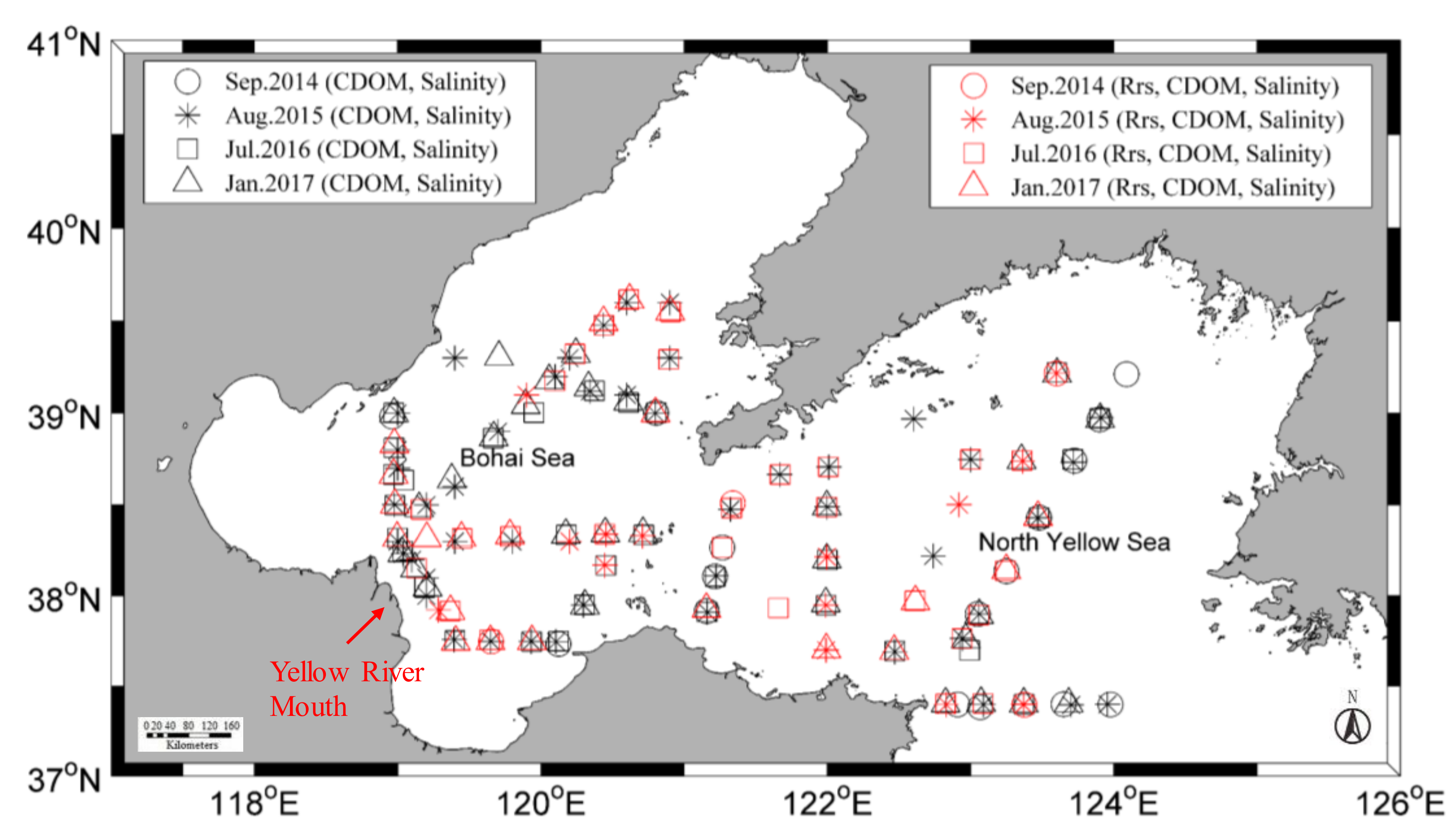
2.1. Study Area and Sampling

The data used in this study were collected from four cruise surveys in the Bohai Sea (BS) and the North Yellow Sea (NYS) (Figure 1). The investigation times were September 2014, August 2015, July 2016 and January 2017.

The Bohai Sea (BS) is an inner sea of China with an area of 77 × 10³ km², an average depth of 18 m, and a maximum depth of 83 m. The North Yellow Sea (NYS) refers to the semi-enclosed sea between the Shandong, Liaodong and Korean peninsulas and has a total surface area of 8 × 10³ km², an average depth of 40 m, and a maximum depth of 86 m. The Yellow River is the major source of freshwater for the BS, while its source of saltwater mainly comes from the Yellow Sea (YS). The sources of freshwater and saltwater change the dynamics of the BS and NYS throughout the Bohai Strait. Due to the uncertainty of bio-optical algorithms in this high-suspended sediment area, it is difficult to obtain reliable ocean color components from the satellite ocean color data [36]. Over the past several decades, the Bohai Sea ecosystem has been gradually deteriorating due to eutrophication [37]. In addition, around the Bohai Strait, there are two main water masses, the Bohai Sea Central Water (BSCW) in the north and the Bohai Sea Coastal Water (BSCoW) in the south [38,39].

2.2. CDOM Measurement

Submersible ECO Fluorometer (Wetlabs Inc., Halifax, NS, Canada) sensors were used to measure the CDOM concentration (C_CDOM), which measures CDOM fluorescence emissions at 460 nm that are excited at 370 nm. The CDOM ECO can obtain CDOM fluorescence across a wide range of water qualities, from mangrove swamps to oligotrophic blue water. The CDOM concentration (ppb) can be calculated by using the equation:

CDOM (ppb) = C_CDOM = Scale Factor × (Output−Dark Counts),

(1)

where Dark Counts indicates the measured signal output in clean water, with black tape over the detector. The Scale Factor (SF) is derived by the following equation, SF = x/(Output-Dark counts), where x is the concentration of the solution used during the instrument characterization. The SF is used to calculate the instrument output concentration from the raw fluorometer signal output.

Another method to characterize CDOM is to measure the absorption coefficient of CDOM (a_CDOM), which was used for comparison with the retrievals in some previous studies. Most of these studies used CDOM absorption as an indicator of CDOM content in their study areas. According to Ocean Optics Protocols Version 2.0, the CDOM samples were collected, stored, and measured [40]. A glass filter system with 0.2 μm polycarbonate filters at a low vacuum less than approximately 125 mmHg was used to obtain the CDOM water samples. The CDOM samples were stored in refrigerators at −20 °C and were measured in the laboratory within 1 month of the cruise. In the laboratory, a Perkin Elmer lambda 650 s ultraviolet–visible light spectrophotometer was used to measure the optical densities (ODs) of the CDOM samples in a 5 cm quartz cell. Milli-Q water was used as the blank, with a flat baseline ±0.0005OD. The CDOM absorption was calculated with:

$$a_{CDOM}\left(\lambda \right)=\left(2.303/l\right)\times \left\{\left[O{D}_{CDOM}\left(\lambda \right)-O{D}_{Milli-Q}\left(\lambda \right)\right]-O{D}_{null}\left({\lambda }_0\right)\right\},$$

(2)

where λ indicates the wavelength of the optic measurement and l indicates the path length of the quartz cell (0.05 m). OD_null(λ₀) is the residual offset at the long wavelength (λ₀), and we used the average values between 695 nm and 705 nm as the residual correction [41]. Note that we only collected the CDOM sample during the cruise in January 2017, and 15 samples from the surface layer of a_CDOM were obtained.

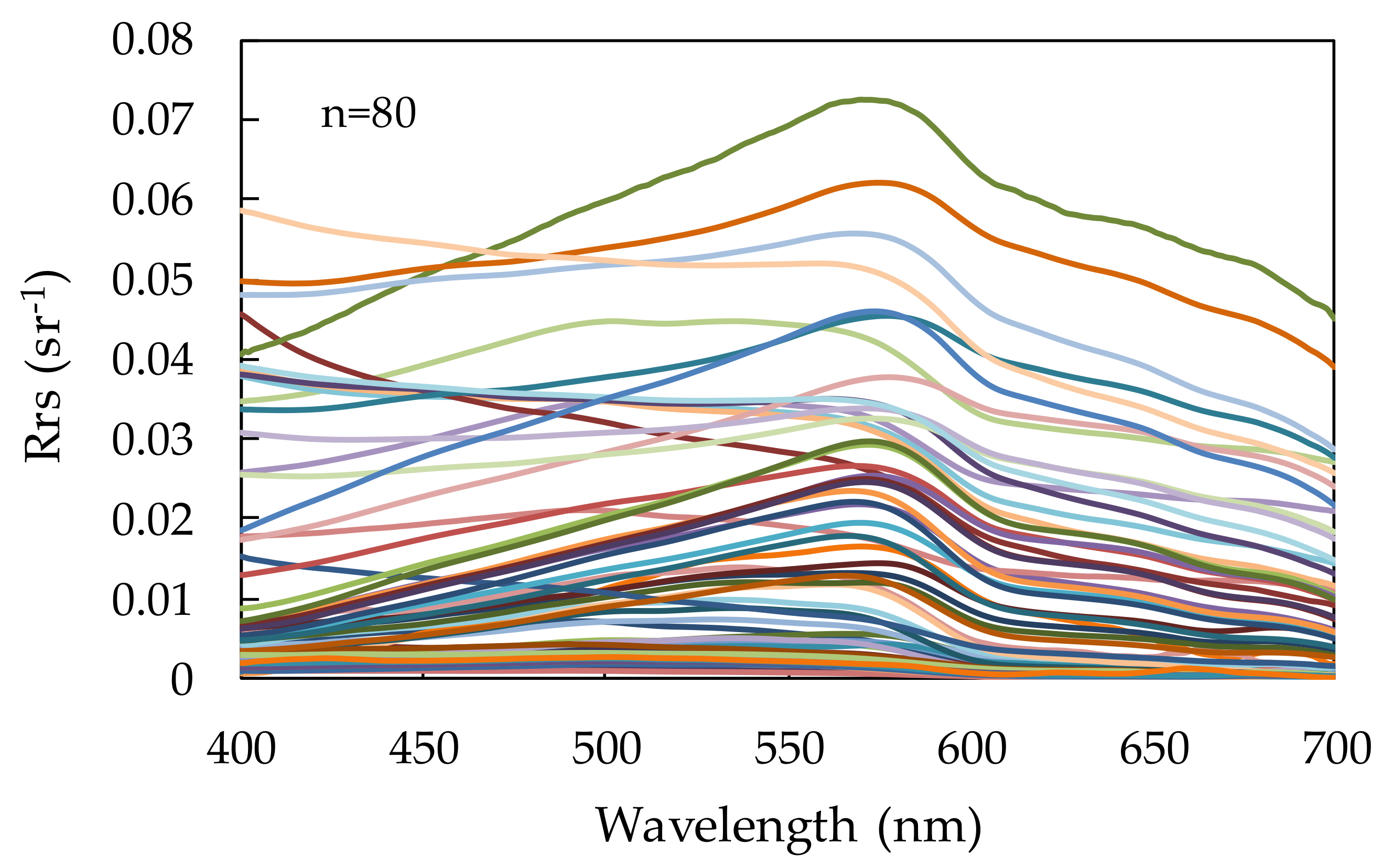
2.3. Spectral Reflectance Measurement

During September 2014, August 2015 and July 2016, remote sensing reflectance (Rrs) values were measured using a Hyper-Profiler II (Satlantic Inc., Halifax, NS, Canada). This instrument has three inter-calibrated radiometers, i.e., a deck sensor that measures the above-water surface down welling irradiance (E_d(λ, 0+)) and two underwater sensors that measure the vertical profiles of down welling irradiance (E_d(λ, z)) and the upwelling radiance (L_u(λ, z)). The instrument covers a spectral range from 349.4 nm to 804.0 nm, with a mean bandwidth of approximately 3.3 nm. The radiometer was down-passed away from the vessel to avoid ship-induced perturbations. Before the instrument drifted away, it was rested on the surface for several minutes to decrease the environmental influence. The processes of calibration, data filtering, binning and interpolation were performed using the manufacturer-provided software Prosoft 7.7.16. To ensure the high quality of the measurements, the data with tilt angles >5° and/or a downward velocity >0.5 m·s⁻¹ were excluded during processing. Rrs (λ) was calculated from

$$Rrs\left(\lambda \right)=\frac{L_W\left(\lambda \right)}{E_d\left(\lambda ,0^{+}\right)},$$

(3)

where E_d(λ, 0+) is the above-water surface down welling irradiance (W m⁻² nm⁻¹), and L_w(λ) is the water-leaving radiance (W m⁻² nm⁻¹ sr⁻¹) derived from the profile of L_u(λ, z) at the upper layer [42]. This method was used to obtain the Rrs spectra in the datasets from September 2014, August 2015, and July 2016.

Another above-water measurement method using an ASD Field spectroradiometer was used in the cruise investigation in January 2017 [43]. The spectroradiometer was used to measure the radiance spectra of the reference panel (L_p), the water (L_t) and the sky (L_sky). Each parameter was sampled more than ten times, and the samples were then averaged as true values. To avoid sun-glint contamination, a zenith angle of 40° and an azimuth angle of 135° were used. Rrs (λ) can be calculated as:

$$R\mathrm{rs}\left(\lambda \right)=\left(L_t-r\times L_{sky}\right)/\left(L_p\times \pi /{\rho }_p\right),$$

(4)

where L_t indicates the radiance from water; L_sky indicates the radiance from the sky; L_p indicates the radiance collected from a reference panel; ρ_p is the diffuse reflectance of the reference panel; and r is the surface Fresnel reflectance, which is a function of wind speed (2.2% for calm weather, 2.5% for <5 m/s wind, 2.6–2.8% for 10 m/s wind) [44].

2.4. Auxiliary Description

A rosette with a Seabird CTD (conductivity–temperature–depth) provided the salinity profiles at each station. During the four cruises, we observed large variability in hydrographical conditions as well as the C_CDOM from coastal to open ocean waters (

Table 1. The distribution of in situ data set and the regression results of the salinity and concentration of colored dissolved organic matter (C_CDOM).

Cruise	Salinity (psu)		CDOM (ppb)		CDOM vs. Salinity
	Min	Max	Min	Max	A	B	R2	P
Sep. 2014 (n = 18)	31.380	32.060	3.226	4.756	-0.522	33.802	0.77	<0.005
Aug. 2015 (n = 80)	29.484	31.963	1.921	8.836	-0.298	32.335	0.80	<0.005
Jul. 2016 (n = 82)	30.367	32.088	2.023	7.822	-0.139	31.989	0.17	<0.005
Jan. 2017 (n = 45)	30.433	32.275	2.538	8.985	-0.058	32.372	0.41	<0.005

The linear regression equation is Y = A × X + B, where Y is the salinity and X is the CDOM concentration. A and B are the slope and the offset, respectively. R² and P are the regression coefficient and the statistically significant coefficient, respectively. Both salinity and CDOM show min and max values, and N is the number of valid samples.

). The Environmental Characterization Optics (ECO) instruments can also measure Chla concentrations. We only used the ECO Chla data for discussing the patterns analyzed in Section 4.1.

The satellite data were downloaded from the NASA ocean color website (https://modis.gsfc.nasa.gov/). In this study, monthly Moderate Resolution Imaging Spectroradiometer (MODIS)/Aqua products of Chla and Rrs at 412 nm, 443 nm, 488 nm and 555 nm sensor bands, with a spatial resolution of approximately 4 km, were used. Furthermore, the daily MODIS/Aqua products of Rrs were also downloaded for the algorithm validation.

We evaluated the performance of algorithms based upon the statistical metrics of the mean absolute percentage difference (APD %), and root mean square error (RMSE) [16,45]. These statistical parameters are expressed as:

$$APD=\frac{1}{N}{\displaystyle \sum _{i=1}^N\left|\frac{P_{\mathrm{ret}}-P_{is}}{P_{is}}\right|}\times 100,$$

(5)

$$RMSE={\left[\frac{1}{N}{\displaystyle \sum _{i=1}^N{\left(P_{\mathrm{ret}}-P_{is}\right)}^2}\right]}^{1/2},$$

(6)

where P_ret, and P_is are algorithm-retrieved values and in situ measured values, respectively.

3. Results

3.1. Description of the In Situ Data Set

In total, 225 samples from the surface layer with C_CDOM (Table 1) and 80 samples from the surface layer with both C_CDOM and in situ Rrs (λ) were obtained (Figure 2). C_CDOM values covered various environments, including the BS and NYS areas, which were used for model development, and the values of C_CDOM varied widely between 1.921 (ppb) to 8.985 (ppb), with an average of 4.430 (ppb) and a standard deviation of 1.935 (ppb).

The collected Rrs spectra in this study are shown in Figure 2. The spectral reflectances were shown to be highly variable and were similar in magnitude to the typical reflectance spectra of the turbid waters [46]. Owing to the phytoplankton pigment and the CDOM absorption, the reflectance was low over 400–500 nm. In particular, in coastal regions such as the BS, the effect of particle absorption will result in a lower down reflectance at 400–500 nm. The peak reflectance at 555 nm is due to weak absorption by phytoplankton and strong scattering by sediment.

C_CDOM showed good correlations with salinity, although different correlation coefficients were present in different cruises (Table 1 and Figure 3). In general, the C_CDOM and salinity were well correlated for all the cruises (Table 1), especially as shown by the seasonal variations.

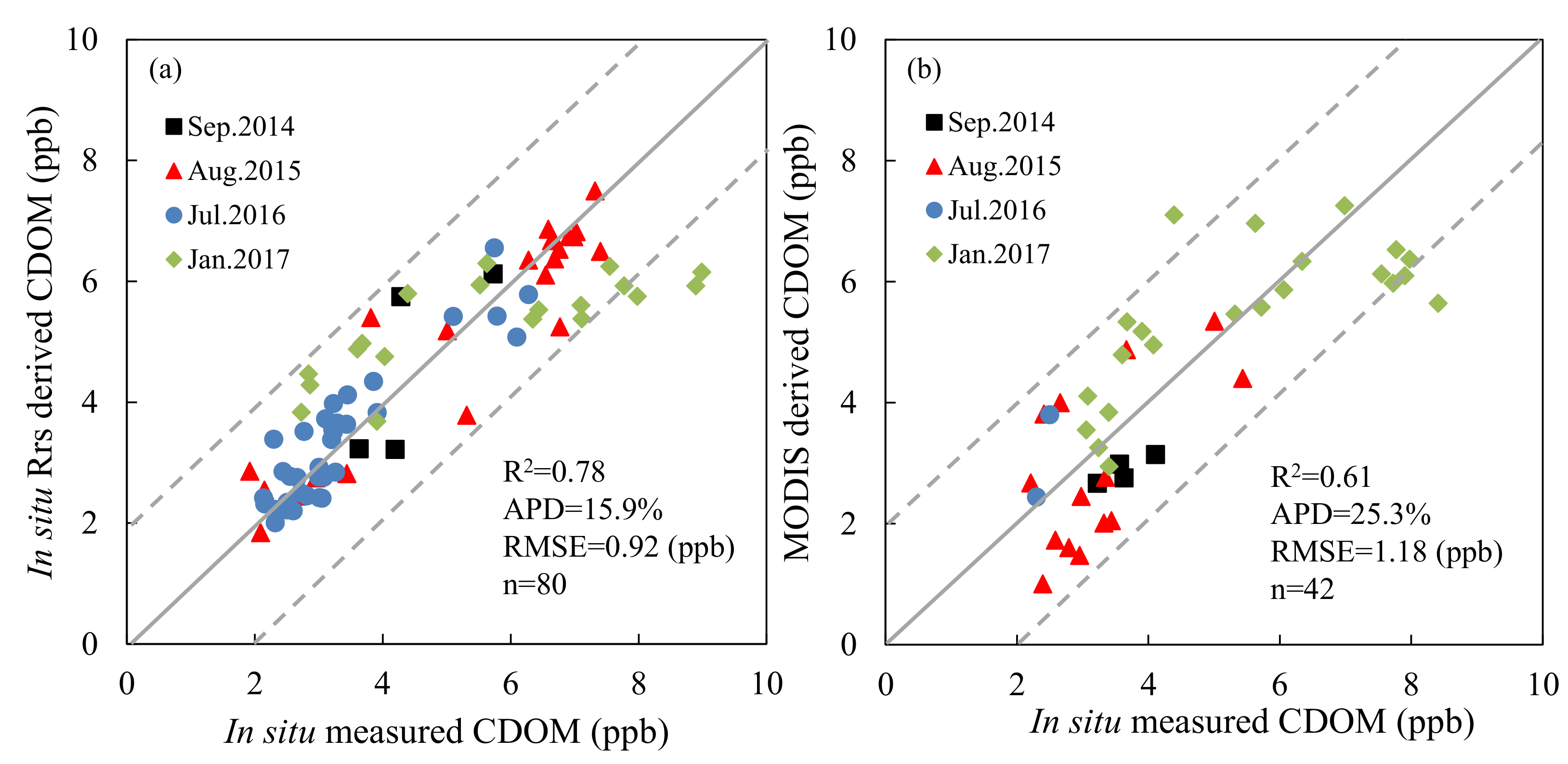
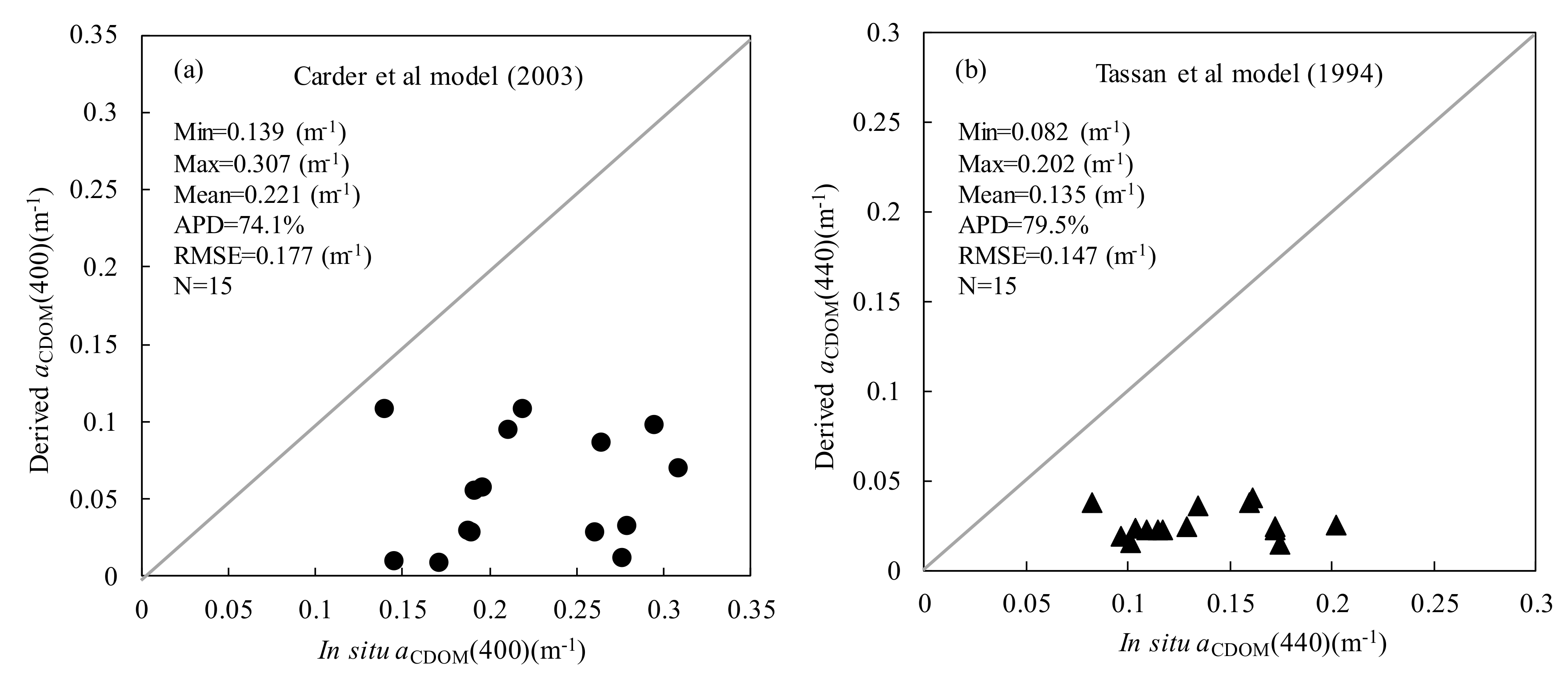
3.2. Development of the CDOM Algorithm

Considering the optical complexity of the studied water regions, this study proposed an empirical region-specific CDOM algorithm. This developed algorithm essentially utilized three band ratios to relate with the CDOM concentration (C_CDOM) based on the following assumptions: (1) reflectances at 412 nm and 443 nm were mostly affected by CDOM [47,48]; (2) reflectances at 488 nm were mostly affected by the phytoplankton, which are a source of CDOM; thus, adding this band into the CDOM algorithm would improve the quantification of photooxidation [9]; and (3) variations in the reflectance near 555 nm was mostly due to suspended particles; thus, adding Rrs(555) may remove the influence of particles [49]. Thus, empirical coefficients of Equation (7) were determined by nonlinear regression with cross-validation by using the in situ data set. The coefficients were the average of all the models.

$$C_{CDOM}(ppb)={10}^{-0.278\left(\frac{R\mathrm{rs}\left(412\right)}{R\mathrm{rs}\left(555\right)}\right)+1.095\left(\frac{R\mathrm{rs}\left(443\right)}{R\mathrm{rs}\left(555\right)}\right)-1.494\left(\frac{R\mathrm{rs}\left(488\right)}{R\mathrm{rs}\left(555\right)}\right)+1.404}$$

(7)

To evaluate the performance and test the robustness of our algorithm for the retrieval of C_CDOM, we conducted a cross-validation [50,51]. In brief, one sample was selected from the full dataset and was used for the model validation. The remaining samples were then used to calibrate the model, and these calibrated models were adapted to derive C_CDOM for the rest of the samples. This procedure was repeated until all of the samples of the full dataset were selected as the validation sample. The estimated C_CDOM obtained from the above steps were independent from each other and formed a new validation dataset. Figure 4a compares the CDOM retrieved using the empirical algorithm with the measured values. As shown in Figure 4a, a strong linear relationship was found between the CDOM and ECO measured values, with an R² value of 0.78, an APD value of 15.9%, and an RMSE value of 0.92 (ppb). The CDOM derived using the MODIS data roughly covaried with the in situ CDOM data. However, as shown in Figure 4b, the derived values of MODIS were somewhat smaller, and the deviation of these values as lower, with an R² value of 0.61, an APD value of 25.3%, and an RMSE value of 1.18 (ppb).

The APD and RMSE of each cross-validation were relatively stable, and most were less than 20% and 0.5 (ppb) (Figures are not shown here). Most CCDOM values ranged from two to eight parts per billion, and when the values were more than 8, the model results showed some bias. The comparisons of the band ratios between the MODIS-derived and the in situ measurements (data not shown) showed MODIS-derived band ratios at 412 nm and 555 nm bands, i.e., the Rrs(412)/Rrs(555) were underestimated, potentially due to poor atmospheric correction at the blue band. Even so, we found that the underestimation of Rrs(412)/Rrs(555) would not produce large errors for the model. To test the effects of three band ratios on the model, we added random errors with a standard deviation of 5–50% and an average value of 0 for Rrs to each band ratio. This process was repeated 1000 times. The APD in the estimations of CDOM increased, with the random errors added to each ratio of Rrs, and the increase rate gradually became larger. Note that the APD of the output errors of Rrs(412)/Rrs(555) is the lowest of the three ratios. In addition, the influence of Rrs(412)/Rrs(555) is lower than the other ratios. Therefore, the ratio of Rrs(412)/Rrs(555) added to our algorithm is reliable, and Rrs(412) is important for the CDOM algorithms. These results indicate that the CCDOM estimation method is robust (data not shown).

In addition to understanding the variations in CDOM, the development of an appropriate satellite algorithm is a key challenge for mapping CDOM using the satellite ocean color data. Here, we tested two typical algorithms for a_CDOM with our in situ data set. To retrieve a_CDOM (400), we tested the algorithm proposed by Carder et al. (2003). This approach has worked well in open ocean and clean shelf waters [52]. The functional form is shown below:

$$\begin{array}{l}{a}_{CDOM}\left(400\right)=1.5\cdot \left[{10}^{-1.147-1.963{\rho }_{15}-1.01{\rho }_{15}^2+0.856{\rho }_{25}+1.702{\rho }_{25}^2}\right]\\ {\rho }_{15}=\frac{Rrs\left(412\right)}{Rrs\left(531\right)},{\rho }_{25}=\frac{Rrs\left(443\right)}{Rrs\left(531\right)}\end{array}.$$

(8)

The other empirical a_CDOM (440) algorithm candidate to be tested was that proposed by Tassan et al. (1994), which worked well in coastal waters [45,53]. The functional form is

$$\begin{array}{l}{a}_{CDOM}\left(440\right)=\left[{10}^{c_1+c_2{\log }_{10}\left(R\right)+c_3{\left({\log }_{10}\left(R\right)\right)}^2}\right]\\ R=\left(\frac{Rrs\left(490\right)}{Rrs\left(555\right)}\right){\left(Rrs\left(443\right)\right)}^{c_0}\\ c_0=0.059,c_1=-0.990,c_2=-1.781,c_3=-2.180\end{array},$$

(9)

where c₀, c₁, c₂ and c₃ are constant coefficients from the work of Siswanto et al. (2011). The algorithm was used by GOCI.

For our in situ data set, the a_CDOM (400) and a_CDOM (440) values from the two algorithms showed a large underestimation of a_CDOM (Figure 5). These classic algorithms did not obtain good results in the BS and NYS. However, our algorithm performed better than these two algorithms (Figure 4).

The underestimation of these algorithms may be caused by regional differences in the optical properties of seawater in the Bohai Sea, which may contain materials that do not co-vary with CDOM, such as chlorophyll pigment and detritus [10,54]. It is worth noting that the data set of a_CDOM was not abundant, but we have an abundant C_CDOM data set. Therefore, we developed an empirical algorithm, which was practical for mapping an entire satellite image with a wide CDOM distribution. Our results suggest that our algorithm is suitable to obtain C_CDOM from the ratios of Rrs(412)/Rrs(555), Rrs(443)/Rrs(555) and Rrs(488)/Rrs(555) with good accuracy. We applied our algorithm to the monthly MODIS/Aqua products of Rrs acquired from 2003 to 2016.

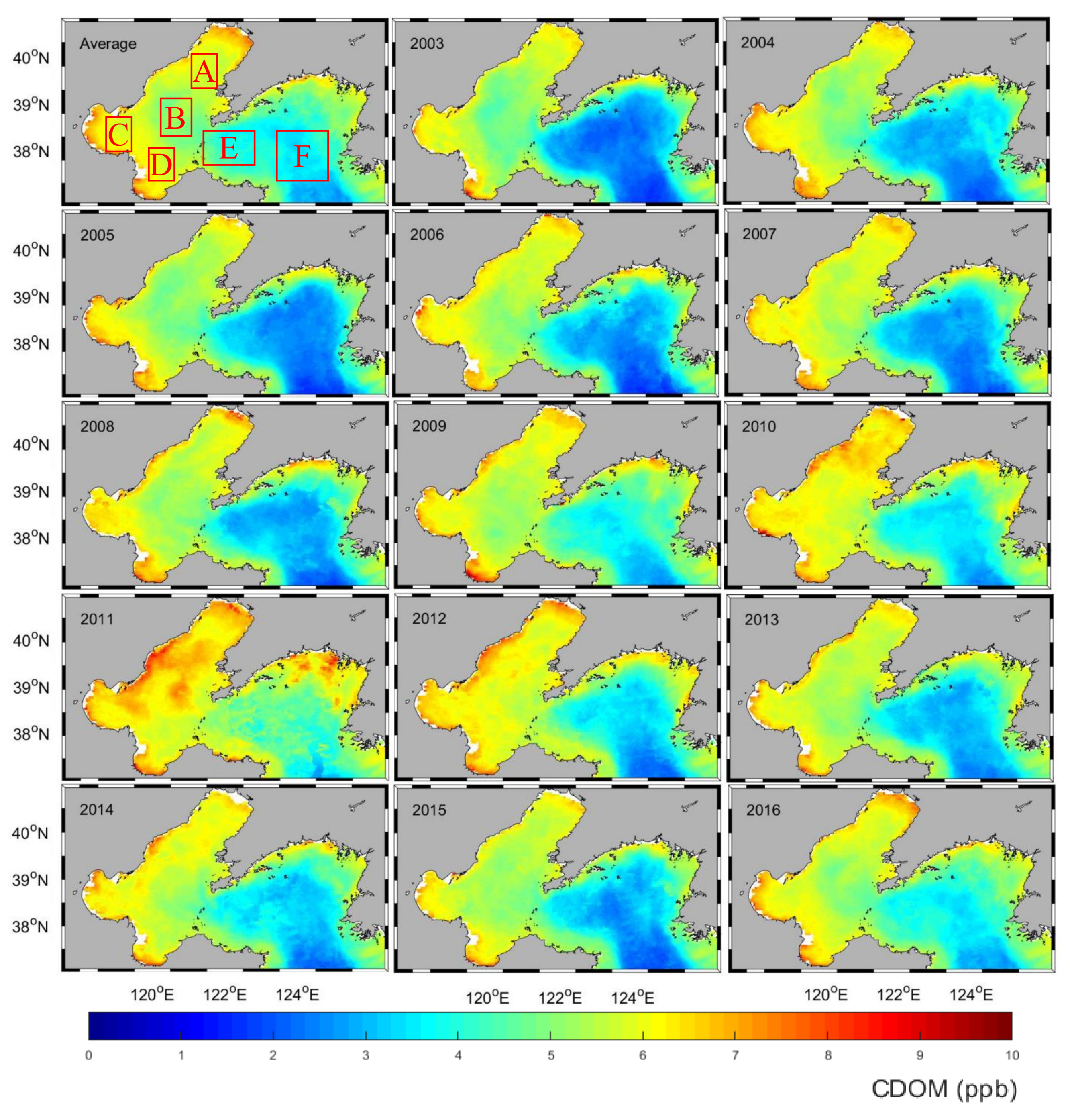
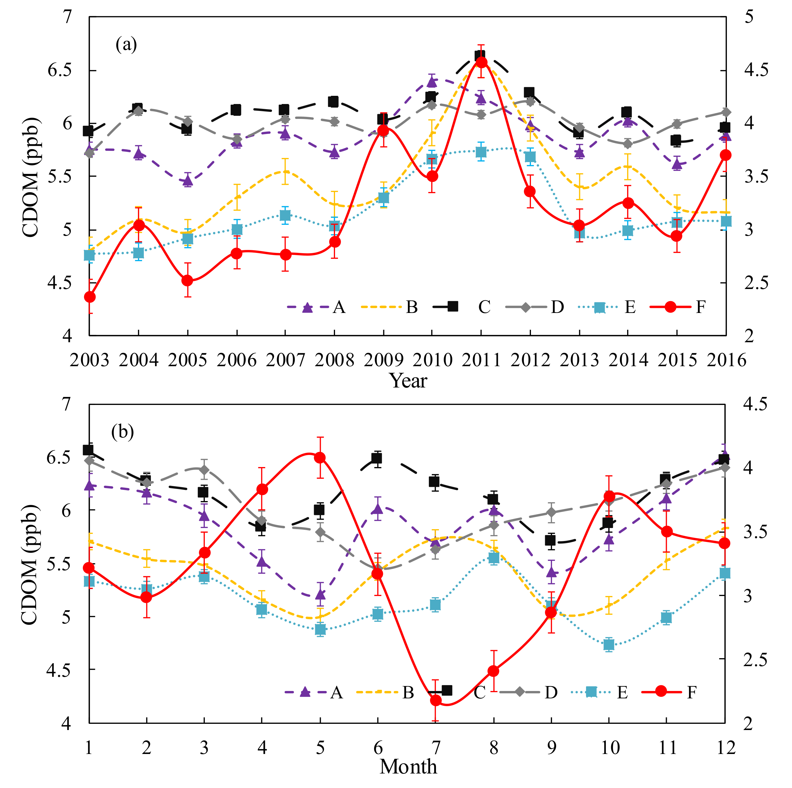
3.3. CDOM Inter-Annual Variability

As shown in Figure 6, there are distinct spatial and annual variations in C_CDOM in the BS and NYS during the period of 2003–2016. High levels of C_CDOM were distributed along the coast of the BS, and a tongue-shaped low-CDOM pattern extended westward to the Bohai Strait. From 2003 to 2011, the C_CDOM significantly increased and then was stable after 2011. In 2011, the C_CDOM showed high distributions in the BS and along the North Korean coast, and a high distribution appeared in the center of the BS. The C_CDOM in some areas of the BS (A, B, C and D) were usually higher than those in other areas (E and F). From 2003 to 2016, the annual average C_CDOM was the highest in the A, C, and D areas (three bays of BS), was relatively low in areas B and E and was the lowest in the F area (Figure 7). This distribution pattern can be divided into three types (Figure 6 and Figure 7a): (1) three bays (A, C and D), where the C_CDOM values were relatively high and had minor variations; (2) the center of the Bohai Sea (B) and the Bohai Strait (E), where the C_CDOM values were lower than those for A, C and D and where the variations were relatively distinct from one another; and (3) the center of the North Yellow Sea (F), where the C_CDOM values were the lowest among the six areas and where the variation was the most significant.

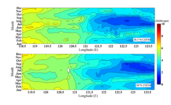
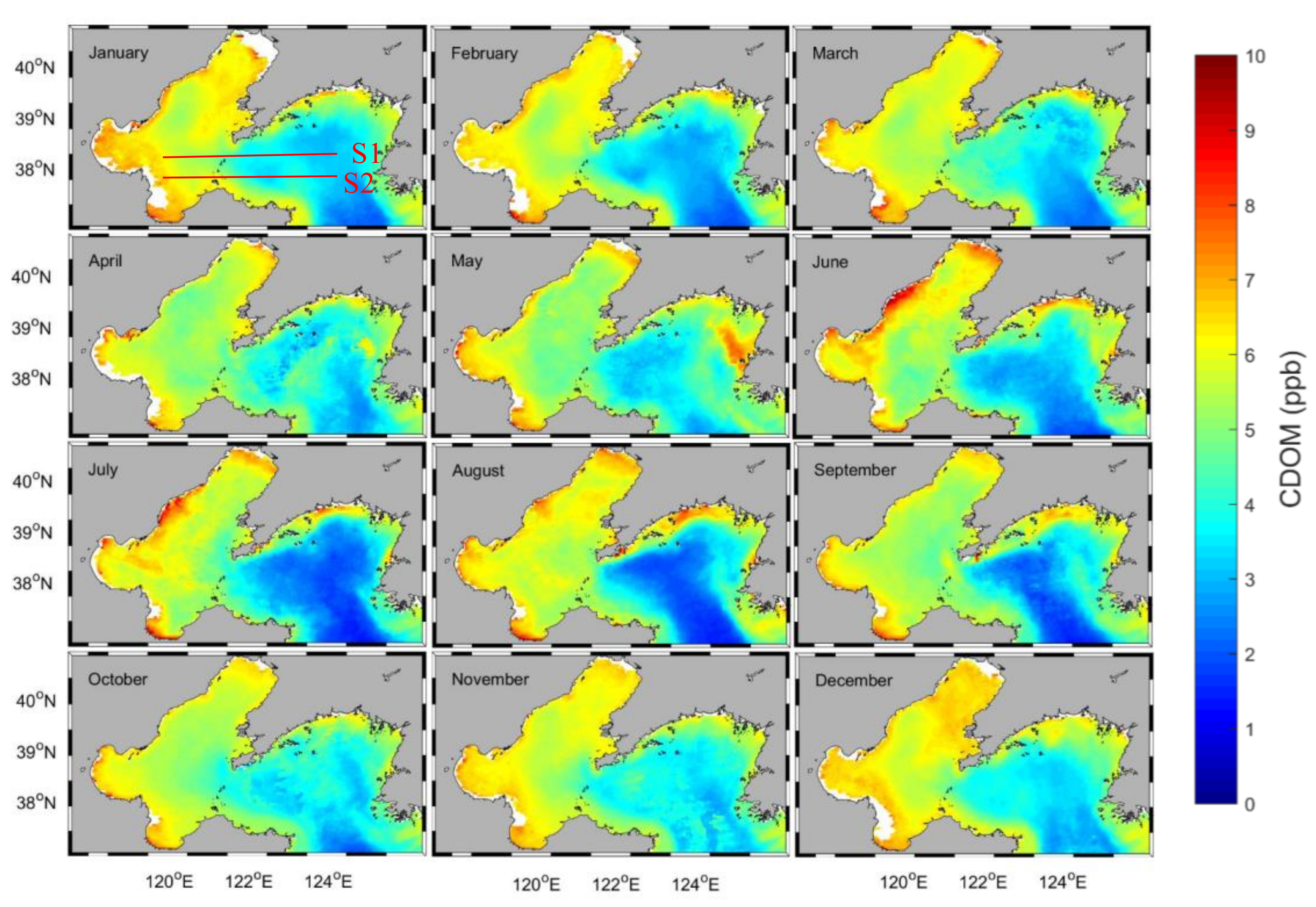
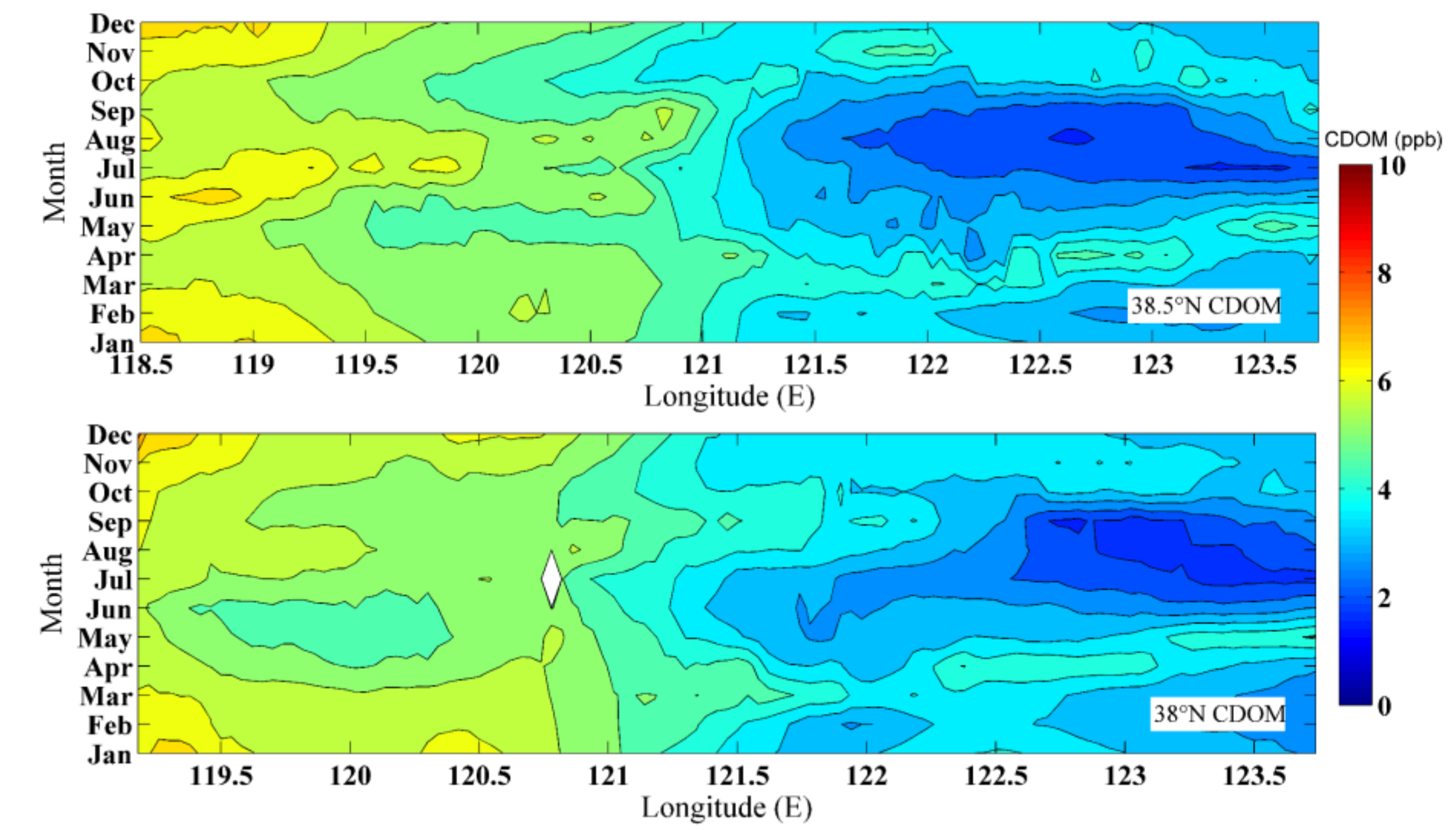
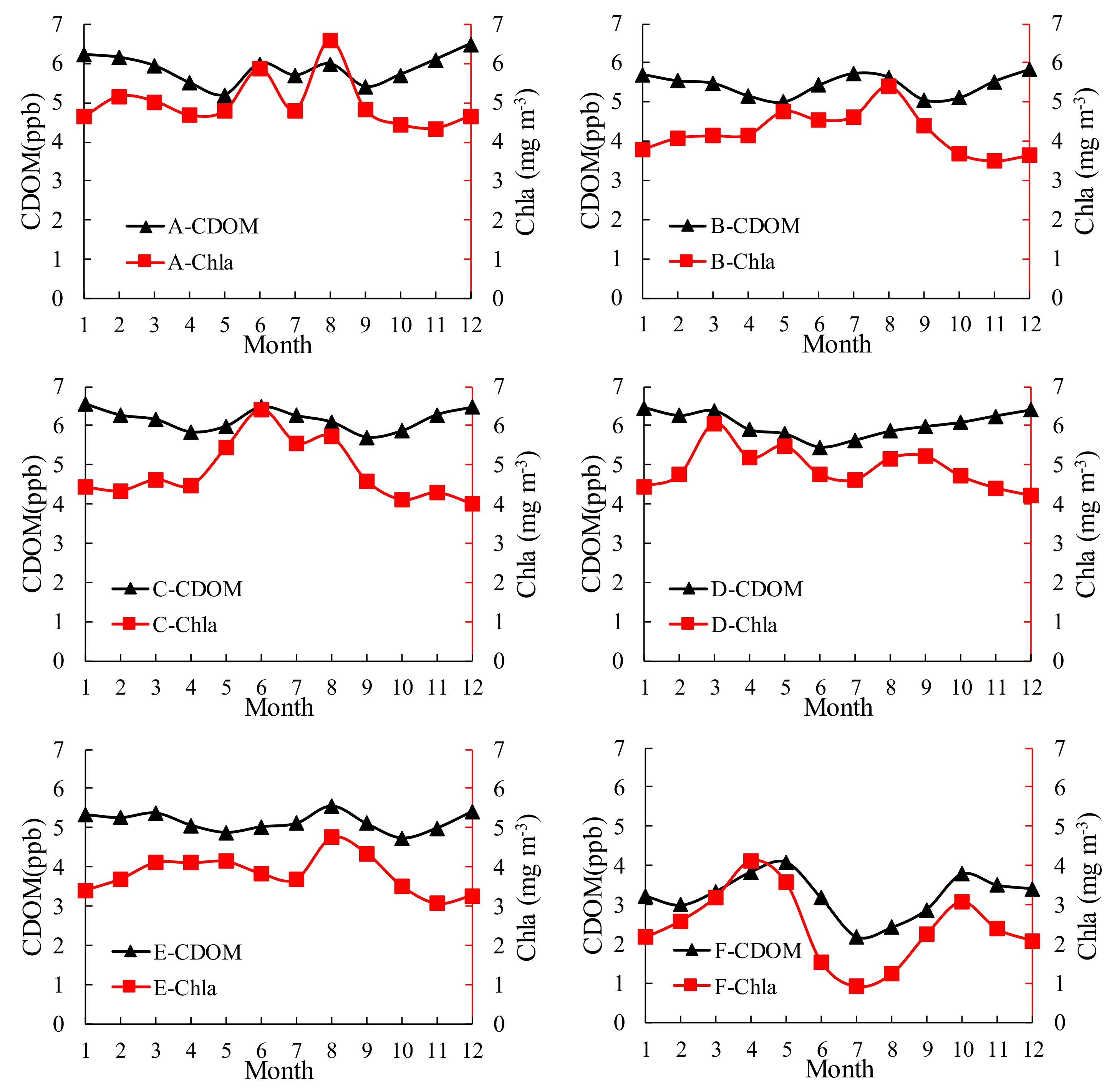
3.4. CDOM Intra-Annual Variability

Monthly averaged C_CDOM values were produced for 14 years. High distributions were seen along the coasts and in the center of the NYS (Figure 8). The C_CDOM in the center of the NYS showed the highest distribution, from March to May, lower values during October to December, and the lowest values from July to September. The C_CDOM values in coastal regions were high during the entire year and were highest in the summer, low in the spring and fall and were the lowest in the winter. The obtained results indicated that the C_CDOM values in the six areas of the study area exhibited different variation trends (Figure 7b). Similar to the C_CDOM values in Section 3.3, this variation can be divided into three types (Figure 7b and Figure 8): (1) in the three bays (A, C and D), the C_CDOM values were relatively high in the summer (June–August) and low in the spring and fall; (2) in the center of the BS (B) and the Bohai Strait (E), the C_CDOM values were the highest in summer, low in the spring and fall and the lowest in the winter; and (3) in the central NYS (F), the C_CDOM values were the highest in the spring and fall, lower in the winter, and lowest in the summer.

Along the 38.5°N latitude line (S1) (118.5–124°E), which covers the central BS to the east of the Bohai Strait, the C_CDOM values were generally high in the west and decreased gradually to the east, with distinct seasonal variations (Figure 9). From March to May, high CDOM values extended to the central NYS. From September to December, the same trend could be observed. Similar to S1, along the 38°N latitude line (S2) (118–124°E), which covers the area from near the Yellow River bank to the east of the Bohai Strait, the 14-year average of monthly CDOM was high from fall to early spring and was low in summer. Over the entire year, a similar tendency was also observed, but the scale extent was low. As shown in Figure 9, along the 38.5°N and 38°N latitude lines, monthly CDOM varied from January to December.

4. Discussion

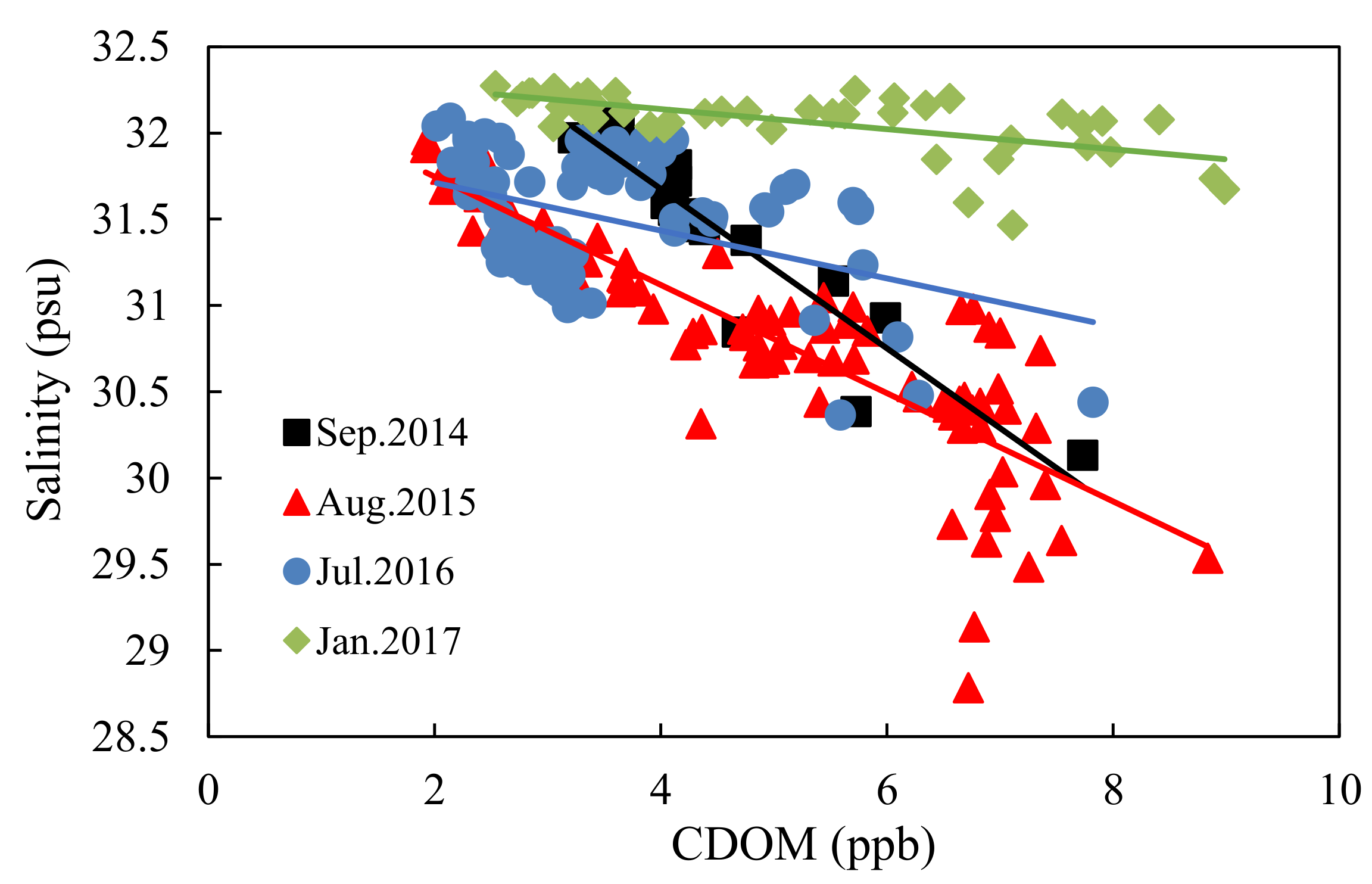
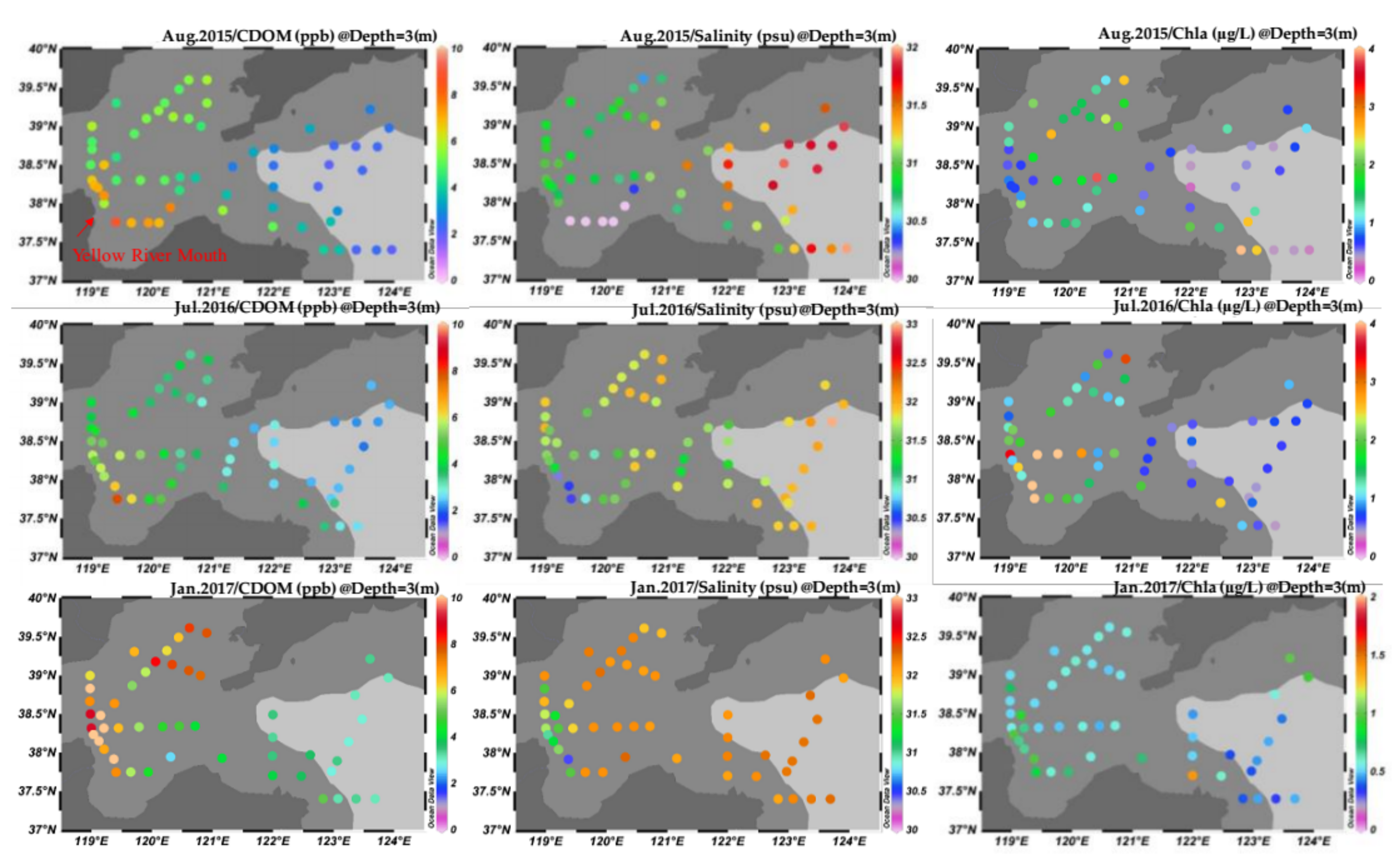
4.1. Explanation of CDOM Patterns Using In Situ Data Sets

C_CDOM showed good correlation with salinity, although different correlation coefficients were present in different cruises (Table 1 and Figure 3). As shown in Figure 10, salinity was low in the near-shore regions (near the mouth of the Yellow River), while the corresponding C_CDOM and Chla concentrations were relatively high in this location. In contrast, in off-shore regions, the salinity was relatively high, while the C_CDOM and Chla concentrations were low.

Strong linear relationships between salinity and CDOM have been found in previous studies [9,21,25,55]. These relationships are likely to be influenced by river discharge, especially near estuaries. There are two sources of CDOM in waters, terrestrial CDOM and autochthonous CDOM. The former’s source is river discharge, while the latter is released as in situ products related to different oceanic phenomena, such as the photosynthetic processes of phytoplankton [56]. Several main rivers, including the Yellow, Haihe, Luanhe and Liaohe rivers, discharge into the BS [57]. Therefore, the obtained strong correlation between salinity and CDOM in the coastal regions of our study area were regarded as being due to terrestrial CDOM discharge [19,20,22].

In contrast to the pattern in the BS and NYS areas, the salinity was low near the mouth of the Yellow River and was closely related to river discharge. Because freshwater discharge from inland rivers carries abundant nutrients, the trophic level in coastal waters increases significantly [58,59]. Thus, increased nutrients may support higher Chla values in coastal waters. In addition to the physical process, there are also chemical and biological processes that influence CDOM distribution [22,60], such as phytoplankton degradation [56] and photochemical bleaching [61].

Generally, C_CDOM values were high in nearshore waters due to physical and chemical processes, and C_CDOM values were lower in the open sea. As shown in Figure 10, more river discharge appeared in nearshore waters, along with high CDOM and Chla values. Higher amounts of river discharge tend to carry more terrestrial CDOM and to export more nutrients into nearshore waters. Thus, high CDOM concentrations along coastal regions were jointly affected by both terrestrial CDOM and autochthonous CDOM. In contrast to the patterns along nearshore waters, there was less river discharge in offshore waters and, thus, low terrestrial CDOM and nutrient content. Correspondingly, this led to low CDOM concentrations in offshore waters.

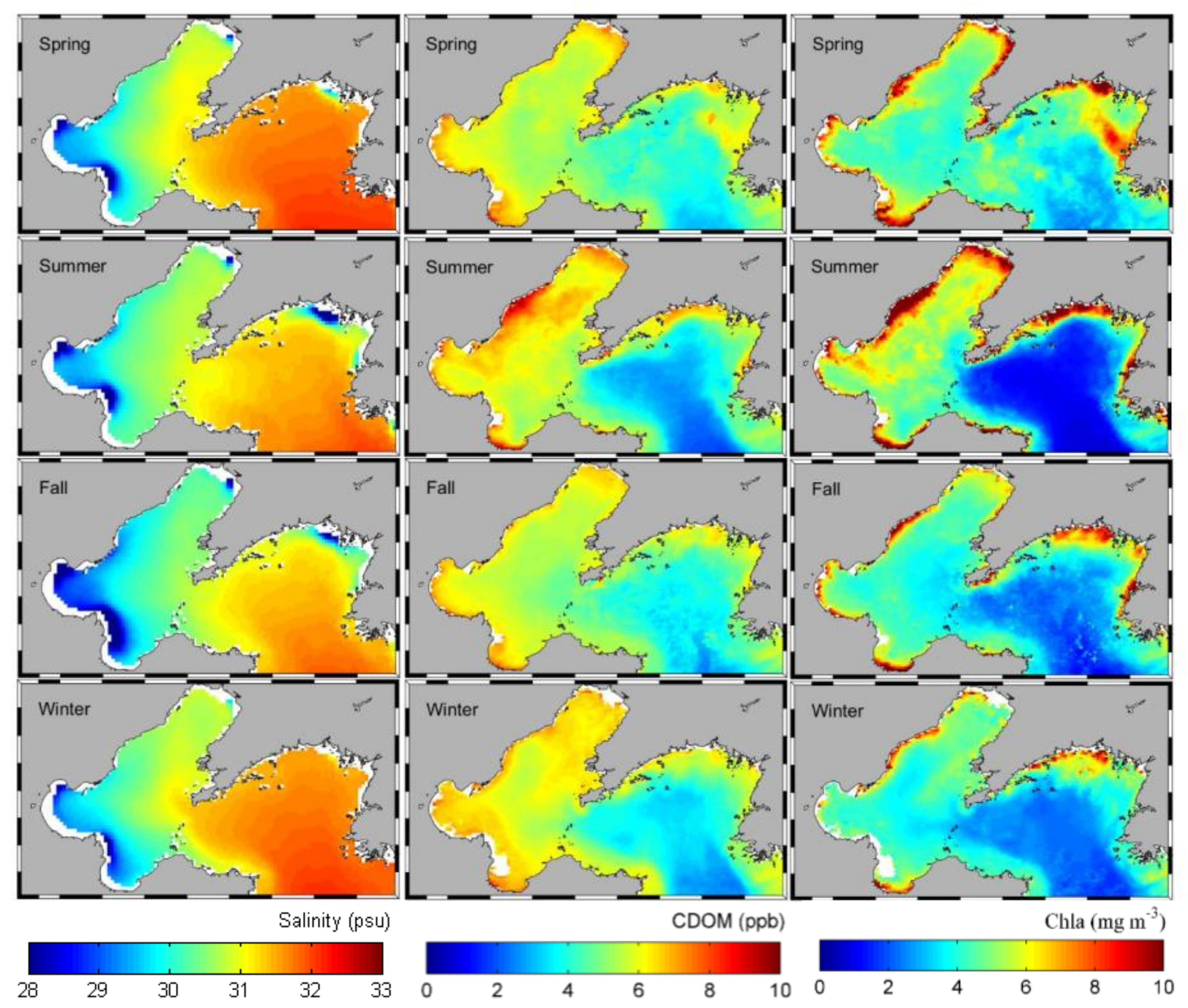
4.2. Explanation of CDOM Patterns Using Satellite- and Model-Derived Data

High CDOM values and correspondingly high Chla values were found in coastal water areas with relatively low salinity. In contrast, low values of CDOM and Chla were found offshore (Figure 10). The satellite-derived CDOM patterns showed agreement with the in situ observed results (Figure 10 and Figure 11). This behavior is probably due to the combined progress of terrestrial CDOM and the degradation of phytoplankton (autochthons CDOM) (see Section 4.1).

Previous studies indicated that phytoplankton blooms could increase CDOM under bloom conditions [62]. Phytoplankton blooms are found regularly during the spring and fall, when the river carries high amounts of terrestrial nutrients and has suitable light and temperature conditions [63,64]. During our study, we observed bloom events during the spring and fall in the east of the Bohai Strait and the central NYS (Figure 11) [65].

Monthly CDOM and Chla values decreased from the BS to NYS (Figure 9). In areas E and F, the CDOM and Chla values showed a similar variation tendency but had different seasonal variations. Correlations between Chla and CDOM were positive in these areas (Figure 12E,F). In areas A, B, C and D, Chla and CDOM exhibited a different variation tendency. Areas E and F are located far from rivers, as discussed above, and areas E and F are mostly influenced by phytoplankton; autochthons CDOM dominated in these areas. In contrast to central NYS, CDOM and Chla in areas A, B, C and D showed different variation tendencies (Figure 12). The fluctuations in CDOM were lower than in areas A and B, as there was a stable source of terrestrial CDOM. However, Chla had a distinct increase tendency during the spring and fall.

The source of CDOM, such as autochthons CDOM additions, can alter C_CDOM values in offshore areas. In offshore waters, the seasonal and spatial differences were remarkable. During the wet season, when the total runoff increased, C_CDOM values in near-shore waters were high, mostly due to the abrupt increase in terrestrial CDOM, while C_CDOM values in offshore waters were low. When one considers the period of phytoplankton blooms (spring and fall), the increase in C_CDOM was clearly observed in the central NYS, a finding regarded as reasonable due to the variation in autochthons CDOM.

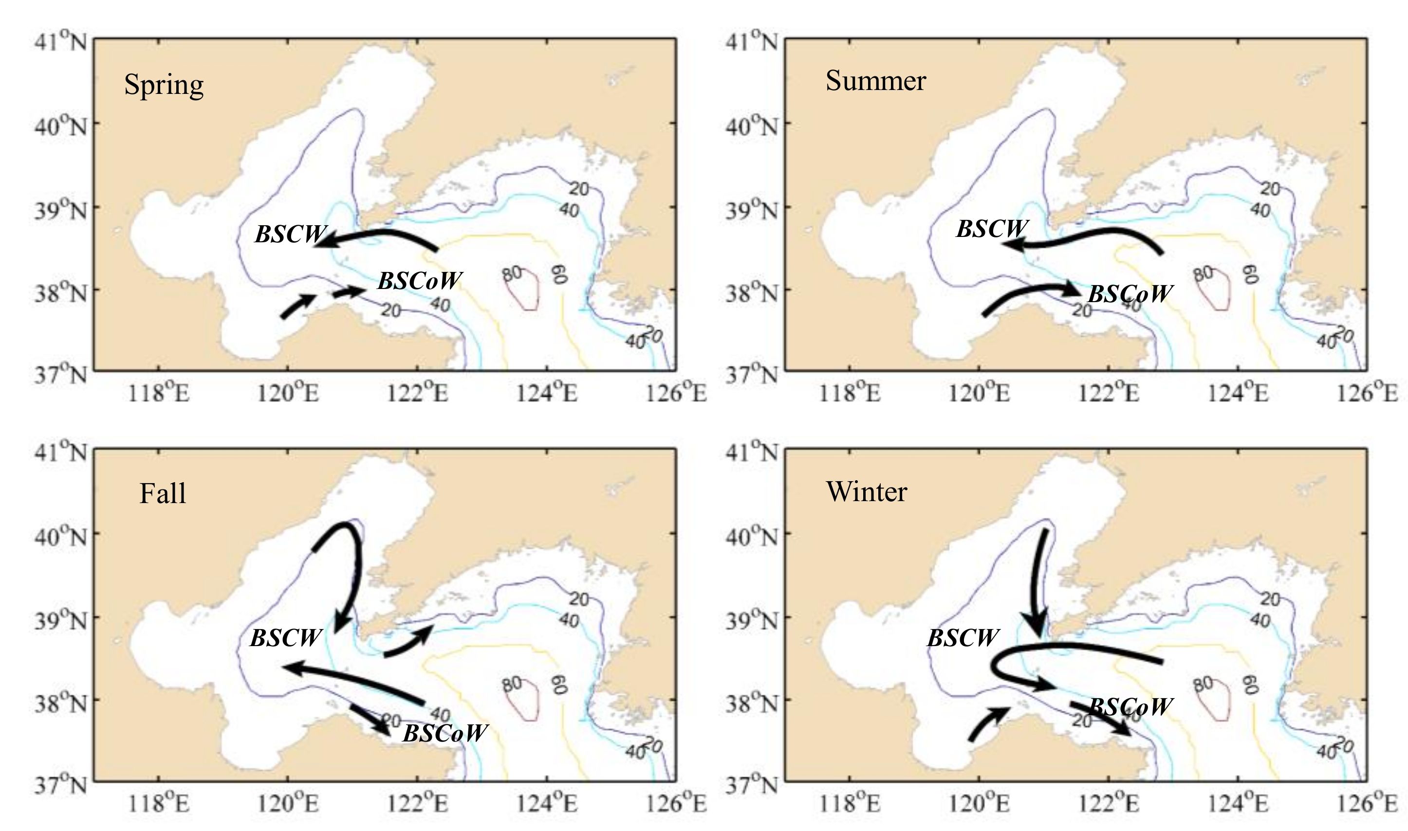
4.3. Influence of Ocean Currents on CDOM Distribution

Apart from the abovementioned influencing factors, ocean currents are also an important driving factor in changing the CDOM distribution [25]. According to previous studies, two main ocean currents exist in the investigated water regions, namely, the Bohai Sea Central Water (BSCW) and the Bohai Sea Coastal Water (BSCoW) [38,57,68]. As shown in Figure 13, the BSCoW moves from the west to the east along the southern coastline of the BS, while the BSCW flows into the BS at the north of the Bohai Strait (except for in winter due to a close cyclonic gyre [68]). The BSCW develops from the Yellow Sea Warm Water and has more saline and poor nutrient levels compared to the BSCoW [39].

Previous studies have found that aquatic biology and hydrodynamic conditions are the main factors related to the spatial and seasonal variations in CDOM [22,24,25]. For example, near the estuary, such as the mouth of the Changjiang River, freshwater discharge from the Changjiang was the dominant factor, which affected the concentration and the spatial and seasonal variations in CDOM [54,55]. Some studies also found complex effects from several water masses in some regions [24,25,60]. Different nutrient conditions carried by ocean currents influenced phytoplankton growth and further changed the CDOM content in waters. For instance, oligotrophic conditions would restrict phytoplankton growth and decrease CDOM content [62,69]. If we assume that the BSCW and BSCoW influence the variations in CDOM, then CDOM would be expected to be high along the BSCoW and low along the BSCW.

Along the latitude lines in this study (S1 and S2, see Figure 7), both C_CDOM and Chla generally decreased from the west to the east (Figure 9 and Figure 11), and they both showed distinct seasonal variations. The 14-year average of the monthly C_CDOM was high from the fall to the early spring, and Chla was high during the spring and fall (Figure 9 and Figure 11). A strong northerly monsoon wind from late November to March influences the study area [39,57], which can increase water column mixing. Nutrients are later carried to the surface, which can support spring phytoplankton blooms in the following year [70]. In addition, the low temperature and instability of the water column make it difficult to support optimal growth conditions for phytoplankton during winter [8].

During the spring (March to May), high C_CDOM extended to central NYS, and Chla exhibited a similar tendency, which indicates that increased C_CDOM existed in central NYS, mostly due to the photochemical processes [3] related to water mass transport. During the fall (September to November), a similar tendency was observed, but its extent and scale were smaller. During the winter, high C_CDOM extended into the NYS through the Bohai Strait, but Chla did not show a similar tendency. This behavior indicated that increased C_CDOM existed in the NYS mostly due to water mass transport. During summer, this phenomenon did not occur.

Overall, the influence of water masses on CDOM is another important factor impacting the variations in CDOM from the east of the BS to the central NYS. A strong relationship was observed between multiyear mean distributions of CDOM and the current field (Figure 13), with high C_CDOM found in the BSCoW areas and low C_CDOM found in the BSCW areas, although C_CDOM varied seasonally. This result is attributable to the fact that the BSCoW not only transports nutrition but also carries a certain amount of CDOM flow into the central NYS. According to the relationship between Chla and CDOM discussed in Figure 11 and Figure 12, we can conclude that the distributions of the multiyear mean CDOM from the west to the east are mainly attributable to currents. Therefore, different water masses with different paths and properties further complicate the variations in CDOM. This complication increases the difficulty of identifying autochthonous CDOM and terrestrial CDOM. Further studies need to provide deeper insight into these CDOM variations.

4.4. Suggestions for Future Work

The findings of this study document long-term CDOM dynamics in the BS and NYS and provide insights into pathways for future improvements. The exposure of CDOM in seawater to solar radiation at all latitudes produces inorganic carbon-based gases, such as carbon dioxide (CO2) and carbon monoxide (CO), which are involved in the variation of dissolved inorganic carbon (DIC) [71,72]. Moreover, CDOM is also the fraction of DOC in seawater, and DOC concentrations are highly correlated with CDOM [73]. In addition to the mechanisms controlling CDOM properties, tracing these variations temporally and geographically is important to better understand the carbon cycle [74].

In contrast, salinity is a direct indicator of a freshwater plume; CDOM, like salinity, is also a soluble matter with distinct values in river and marine end-members [19]. In many river estuaries and plume systems, CDOM shows good negative correlations with salinity [21,24,54,55]. Therefore, in recent years, CDOM derived from the satellite ocean color data has been used to estimate salinities in coastal waters [10,19,20]. A simple negative linear relationship between CDOM and salinity was also observed in the current study. However, the relationships between CDOM and salinity have distinct local variable features among different freshwater and marine ecosystems and are influenced by regional hydrodynamic and biogeochemical processes [25]. Therefore, it is generally practical to apply a locally stable salinity–CDOM relationship to water areas of interest using sufficient regional field measurements, which then serve for documenting long-term salinity changes.

In short, the findings of this study demonstrate that the long-term monitoring of CDOM dynamics has important marine biogeochemical and environmental implications. This study will provide a potentially efficient indicator of marine ecosystem variations and will serve as a tool for managing and protecting marine environments in response to future climate change.

5. Conclusions

This study developed a regional empirical remote sensing approach to estimate C_CDOM in the BS and NYS areas. The designed algorithm uses the ratios of Rrs(412)/Rrs(555), Rrs(443)/Rrs(555) and Rrs(488)/Rrs(555). Both in situ and satellite validations had good performance, with R² values of 0.78 and 0.61, RMSE values of 0.92 (ppb) and 1.18 (ppb), and APD values of 15.9% and 25.3%, respectively. A long-term MODIS-derived CDOM pattern during the period of 2003–2016 was obtained, indicating its inter/intra-annual variations. From 2003 to 2011, the C_CDOM values significantly increased and were stable after 2011. In 2011, the C_CDOM values had high distributions in the BS. High C_CDOM values were observed in coastal waters, and these values gradually decreased when moving from the BS to NYS. During the summer, C_CDOM was relatively high in nearshore waters due to a large amount of terrestrial CDOM discharge. During the spring and fall, the C_CDOM values were higher in central NYS, mostly due to phytoplankton blooms.

During the winter, C_CDOM was relatively high in the three bays of the BS. In the nearshore waters, the CDOM was mainly affected by terrestrial CDOM from river discharge, while the photochemical process dominated and changed C_CDOM in offshore waters. Furthermore, the annual mean distribution patterns of CDOM shown in the BS and NYS areas were mainly attributable to ocean currents. Overall, the findings demonstrated here have significant implications for the long-term variation in aquatic environments.

References

1. Herzsprung, P.; Von TüMpling, W.; Hertkorn, N.; Harir, M.; BüTtner, O.; Bravidor, J.; Friese, K.; Schmitt-Kopplin, P. Variations of DOM quality in inflows of a drinking water reservoir: Linking of van Krevelen diagrams with EEMF spectra by rank correlation. Environ. Sci. Technol. 2012, 46, 5511–5518. [Google Scholar] [CrossRef] [PubMed]
2. Evans, C.D.; Monteith, D.T.; Cooper, D.M. Long-term increases in surface water dissolved organic carbon: Observations, possible causes and environmental impacts. Environ. Pollut. 2005, 137, 55–71. [Google Scholar] [CrossRef] [PubMed]
3. Brezonik, P.L.; Olmanson, L.G.; Finlay, J.C.; Bauer, M.E. Factors affecting the measurement of CDOM by remote sensing of optically complex inland waters. Remote Sens. Environ. 2015, 157, 199–215. [Google Scholar] [CrossRef]
4. Del Castillo, C.E.; Coble, P.G.; Morell, J.M.; López, J.M.; Corredor, J.E. Analysis of the optical properties of the Orinoco River plume by absorption and fluorescence spectroscopy. Mar. Chem. 1999, 66, 35–51. [Google Scholar] [CrossRef]
5. Mannino, A.; Russ, M.E.; Hooker, S.B. Algorithm development and validation for satellite-derived distributions of DOC and CDOM in the US Middle Atlantic Bight. J. Geophys. Res. Oceans 2008, 113. [Google Scholar] [CrossRef]
6. Doney, S.C.; Najjar, R.G.; Stewart, S. Photochemistry, mixing and diurnal cycles in the upper ocean. J. Mar. Res. 1995, 53, 341–369. [Google Scholar] [CrossRef]
7. D’sa, E.J.; Miller, R.L.; Del Castillo, C. Bio-optical properties and ocean color algorithms for coastal waters influenced by the Mississippi River during a cold front. Appl. Opt. 2006, 45, 7410–7428. [Google Scholar] [CrossRef] [PubMed]
8. Yamada, K.; Ishizaka, J.; Yoo, S.; Kim, H.-C.; Chiba, S. Seasonal and interannual variability of sea surface chlorophyll a concentration in the Japan/East Sea (JES). Prog. Oceanogr. 2004, 61, 193–211. [Google Scholar] [CrossRef]
9. Bélanger, S.; Babin, M.; Larouche, P. An empirical ocean color algorithm for estimating the contribution of chromophoric dissolved organic matter to total light absorption in optically complex waters. J. Geophys. Res. Atmos. 2008, 113, 977–990. [Google Scholar] [CrossRef]
10. Ahn, Y.; Shanmugam, P.; Moon, J.; Ryu, J.-H. Satellite Remote Sensing of a Low-Salinity Water Plume in the East China Sea; Annales Geophysicae; Copernicus GmbH: Gottingen, Germany, 2008; pp. 2019–2035. [Google Scholar]
11. Joshi, I.; D’sa, E.J. Seasonal variation of colored dissolved organic matter in Barataria Bay, Louisiana, using combined Landsat and field data. Remote Sens. 2015, 7, 12478–12502. [Google Scholar] [CrossRef]
12. Cao, F.; Tzortziou, M.; Hu, C.; Mannino, A.; Fichot, C.G.; Del Vecchio, R.; Najjar, R.G.; Novak, M. Remote sensing retrievals of colored dissolved organic matter and dissolved organic carbon dynamics in North American estuaries and their margins. Remote Sens. Environ. 2018, 205, 151–165. [Google Scholar] [CrossRef]
13. Lee, Z. Reports of the International Ocean-Colour Coordinating Group; IOCCG: Dartmouth, NS, Canada, 2006; Available online: http://ioccg.org/wp-content/uploads/2016/02/report3.pdf (accessed on 24 April 2018).
14. Zhu, W.; Yu, Q.; Tian, Y.Q.; Chen, R.F.; Gardner, G.B. Estimation of chromophoric dissolved organic matter in the Mississippi and Atchafalaya river plume regions using above-surface hyperspectral remote sensing. J. Geophys. Res. Atmos. 2010, 116, 434–441. [Google Scholar] [CrossRef]
15. Lee, Z.; Carder, K.L.; Arnone, R.A. Deriving inherent optical properties from water color: A multiband quasi-analytical algorithm for optically deep waters. Appl. Opt. 2002, 41, 5755–5772. [Google Scholar] [CrossRef] [PubMed]
16. Zhu, W.; Yu, Q.; Tian, Y.Q.; Becker, B.L.; Zheng, T.; Carrick, H.J. An assessment of remote sensing algorithms for colored dissolved organic matter in complex freshwater environments. Remote Sens. Environ. 2014, 140, 766–778. [Google Scholar] [CrossRef]
17. Sathyendranath, S. Remote Sensing of Ocean Colour in Coastal, and Other Optically-Complex, Waters; IOCCG report 2000; IOCCG: Dartmouth, NS, Canada; Available online: http://ioccg.org/wp-content/uploads/2016/02/report3.pdf (accessed on 24 April 2018).
18. Brando, V.E.; Dekker, A.G. Satellite hyperspectral remote sensing for estimating estuarine and coastal water quality. IEEE Trans. Geosci. Remote Sens. 2003, 41, 1378–1387. [Google Scholar] [CrossRef]
19. Siddorn, J.R.; Bowers, D.G.; Hoguane, A.M. Detecting the Zambezi River Plume using Observed Optical Properties. Mar. Pollut. Bull. 2001, 42, 942–950. [Google Scholar] [CrossRef]
20. Binding, C.E.; Bowers, D.G. Measuring the salinity of the Clyde Sea from remotely sensed ocean colour. Estuar. Coast. Shelf Sci. 2003, 57, 605–611. [Google Scholar] [CrossRef]
21. Bowers, D.G.; Brett, H.L. The relationship between CDOM and salinity in estuaries: An analytical and graphical solution. J. Mar. Syst. 2008, 73, 1–7. [Google Scholar] [CrossRef]
22. Vecchio, R.D.; Blough, N.V. Spatial and seasonal distribution of chromophoric dissolved organic matter and dissolved organic carbon in the Middle Atlantic Bight. Mar. Chem. 2004, 89, 169–187. [Google Scholar] [CrossRef]
23. Bricaud, A.; Babin, M.; Claustre, H.; Ras, J.; Tièche, F. Light absorption properties and absorption budget of Southeast Pacific waters. J. Geophys. Res. Oceans 2010, 115. [Google Scholar] [CrossRef]
24. Stedmon, C.A.; Osburn, C.L.; Kragh, T. Tracing water mass mixing in the Baltic–North Sea transition zone using the optical properties of coloured dissolved organic matter. Estuar. Coast. Shelf Sci. 2010, 87, 156–162. [Google Scholar] [CrossRef]
25. Matsuoka, A.; Bricaud, A.; Benner, R.; Para, J.; Sempéré, R.; Prieur, L.; Bélanger, S.; Babin, M. Tracing the transport of colored dissolved organic matter in water masses of the Southern Beaufort Sea: Relationship with hydrographic characteristics. Biogeosci. Discuss. 2012, 8, 925–940. [Google Scholar] [CrossRef]
26. Matsuoka, A.; Hooker, S.B.; Bricaud, A.; Gentili, B.; Babin, M. Estimating absorption coefficients of colored dissolved organic matter (CDOM) using a semi-analytical algorithm for southern Beaufort Sea waters: Application to deriving concentrations of dissolved organic carbon from space. Biogeosciences 2013, 10, 917–927. [Google Scholar] [CrossRef]
27. Blough, N.; Zafiriou, O.; Bonilla, J. Optical absorption spectra of waters from the Orinoco River outflow: Terrestrial input of colored organic matter to the Caribbean. J. Geophys. Res. Oceans 1993, 98, 2271–2278. [Google Scholar] [CrossRef]
28. Vecchio, R.D.; Blough, N.V. Photobleaching of chromophoric dissolved organic matter in natural waters: Kinetics and modeling. Mar. Chem. 2002, 78, 231–253. [Google Scholar] [CrossRef]
29. Vodacek, A.; Blough, N.V.; Degrandpre, M.D.; Peltzer, E.T.; Nelson, R.K. Seasonal variation of CDOM and DOC in the Middle Atlantic Bight: Terrestrial inputs and photooxidation. Limnol. Oceanogr. 1997, 42, 674–686. [Google Scholar] [CrossRef]
30. Moran, M.A.; Sheldon, W.M.; Zepp, R.G. Carbon loss and optical property changes during long-term photochemical and biological degradation of estuarine dissolved organic matter. Limnol. Oceanogr. 2000, 45, 1254–1264. [Google Scholar] [CrossRef]
31. Kowalczuk, P.; Cooper, W.J.; Whitehead, R.F.; Durako, M.J.; Sheldon, W. Characterization of CDOM in an organic-rich river and surrounding coastal ocean in the South Atlantic Bight. Aquat. Sci. 2003, 65, 384–401. [Google Scholar] [CrossRef]
32. Stedmon, C.A.; Markager, S. Behaviour of the optical properties of coloured dissolved organic matter under conservative mixing. Estuar. Coast. Shelf Sci. 2003, 57, 973–979. [Google Scholar] [CrossRef]
33. Li, G.; Liu, J.; Ma, Y.; Zhao, R.; Hu, S.; Li, Y.; Wei, H.; Xie, H. Distribution and spectral characteristics of chromophoric dissolved organic matter in a coastal bay in northern China. J. Environ. Sci. 2014, 26, 1585–1595. [Google Scholar] [CrossRef] [PubMed]
34. Kowalczuk, P.; Durako, M.J.; Young, H.; Kahn, A.E.; Cooper, W.J.; Gonsior, M. Characterization of dissolved organic matter fluorescence in the South Atlantic Bight with use of PARAFAC model: Interannual variability. Mar. Chem. 2009, 113, 182–196. [Google Scholar] [CrossRef]
35. Bai, Y.; Su, R.; Yao, Q.; Zhang, C.; Shi, X. Characterization of Chromophoric Dissolved Organic Matter (CDOM) in the Bohai Sea and the Yellow Sea Using Excitation-Emission Matrix Spectroscopy (EEMs) and Parallel Factor Analysis (PARAFAC). Estuar. Coasts 2017, 40, 1325–1345. [Google Scholar] [CrossRef]
36. Jamet, C.; Loisel, H.; Kuchinke, C.P.; Ruddick, K.; Zibordi, G.; Feng, H. Comparison of three SeaWiFS atmospheric correction algorithms for turbid waters using AERONET-OC measurements. Remote Sens. Environ. 2011, 115, 1955–1965. [Google Scholar] [CrossRef]
37. Peng, S. The nutrient, total petroleum hydrocarbon and heavy metal contents in the seawater of Bohai Bay, China: Temporal–spatial variations, sources, pollution statuses, and ecological risks. Mar. Pollut. Bull. 2015, 95, 445–451. [Google Scholar] [CrossRef] [PubMed]
38. Su, Y.S.; Weng, X.C. Water Masses in China Seas; Springer Netherlands: Berlin, Germany, 1994; pp. 3–16. [Google Scholar]
39. Chen, C.T.A. Chemical and physical fronts in the Bohai, Yellow and East China seas. J. Mar. Syst. 2009, 78, 394–410. [Google Scholar] [CrossRef]
40. Mitchell, B.G.; Kahru, M.; Wieland, J.; Stramska, M. Determination of spectral absorption coefficients of particles, dissolved material and phytoplankton for discrete water samples. Ocean optics protocols for satellite ocean color sensor validation. Revision 2002, 3, 231. [Google Scholar]
41. Babin, M.; Stramski, D.; Ferrari, G.M.; Claustre, H.; Bricaud, A.; Obolensky, G.; Hoepffner, N. Variations in the light absorption coefficients of phytoplankton, nonalgal particles, and dissolved organic matter in coastal waters around Europe. J. Geophys. Res. Oceans 2003, 108. [Google Scholar] [CrossRef]
42. Hirawake, T.; Takao, S.; Horimoto, N.; Ishimaru, T.; Yamaguchi, Y.; Fukuchi, M. A phytoplankton absorption-based primary productivity model for remote sensing in the Southern Ocean. Polar Biol. 2011, 34, 291–302. [Google Scholar] [CrossRef]
43. Mueller, J.; Morel, A.; Frouin, R.; Davis, C.; Arnone, R.; Carder, K.; Lee, Z.; Steward, R.; Hooker, S.; Mobley, C. Ocean optics protocols for Satellite Ocean Color validation, Revision 4, Volume III: Radiometric Measurements and Data Analysis Protocols; Mueller, J.L., Fargion, G.S., McClain, C.R., Eds.; NASA/TM: Greenbelt, MD, USA, 2003; p. 21621. [Google Scholar]
44. Lee, Z.; Carder, K.; Steward, R.; Peacock, T.; Davis, C.; Mueller, J. Protocols for Measurement of Remote-Sensing Reflectance from Clear to Turbid Waters; SeaWiFS Workshop: Halifax, NS, Canada, 1996. [Google Scholar]
45. Siswanto, E.; Tang, J.; Yamaguchi, H.; Ahn, Y.H. Empirical ocean-color algorithms to retrieve chlorophyll-a, total suspended matter, and colored dissolved organic matter absorption coefficient in the Yellow and East China Seas. J. Oceanogr. 2011, 67, 627–650. [Google Scholar] [CrossRef]
46. Gitelson, A.A.; Schalles, J.F.; Hladik, C.M. Remote chlorophyll—A retrieval in turbid, productive estuaries: Chesapeake Bay case study. Remote Sens. Environ. 2007, 109, 464–472. [Google Scholar] [CrossRef]
47. Del Castillo, C.E.; Coble, P.G. Seasonal variability of the colored dissolved organic matter during the 1994–95 NE and SW monsoons in the Arabian Sea. Deep Sea Res. Part II Top. Stud. Oceanogr. 2000, 47, 1563–1579. [Google Scholar] [CrossRef]
48. Sun, D.Y.; Li, Y.M.; Wang, Q.; Lu, H.; Le, C.F.; Huang, C.C.; Gong, S.Q. A neural-network model to retrieve CDOM absorption from in situ measured hyperspectral data in an optically complex lake: Lake Taihu case study. Int. J. Remote Sens. 2011, 32, 4005–4022. [Google Scholar] [CrossRef]
49. Ouillon, S.; Douillet, P.; Petrenko, A.; Neveux, J.; Dupouy, C.; Froidefond, J.-M.; Andréfouët, S.; Muñoz-Caravaca, A. Optical algorithms at satellite wavelengths for total suspended matter in tropical coastal waters. Sensors 2008, 8, 4165–4185. [Google Scholar] [CrossRef] [PubMed]
50. Kohavi, R. A Study of Cross-Validation and Bootstrap for Accuracy Estimation and Model Selection. In Proceedings of the International Joint Conference on Artificial Intelligence, Montreal, QC, Canada, 20–25 August 1995; pp. 1137–1143. [Google Scholar]
51. Wang, S.; Yu, H.; Qiu, Z.; Sun, D.; Zhang, H.; Zheng, L.; Xiao, C. Remote Sensing of Particle Cross-Sectional Area in the Bohai Sea and Yellow Sea: Algorithm Development and Application Implications. Remote Sens. 2016, 8, 841. [Google Scholar] [CrossRef]
52. Carder, K.L.; Chen, F.R.; Lee, Z.; Hawes, S.K.; Cannizzaro, J.P. MODIS ocean science team algorithm theoretical basis document. ATBD 2003, 19, 7–18. [Google Scholar]
53. Tassan, S. Local algorithms using SeaWiFS data for the retrieval of phytoplankton, pigments, suspended sediment, and yellow substance in coastal waters. Appl. Opt. 1994, 33, 2369–2378. [Google Scholar] [CrossRef] [PubMed]
54. Sasaki, H.; Siswanto, E.; Kou, N.; Tanaka, K.; Hasegawa, T.; Ishizaka, J. Mapping the low salinity Changjiang Diluted Water using satellite-retrieved colored dissolved organic matter (CDOM) in the East China Sea during high river flow season. Geophys. Res. Lett. 2008, 35, 121–134. [Google Scholar] [CrossRef]
55. Bai, Y.; Pan, D.; Cai, W.J.; He, X.; Wang, D.; Tao, B.; Zhu, Q. Remote sensing of salinity from satellite-derived CDOM in the Changjiang River dominated East China Sea. J. Geophys. Res. Oceans 2013, 118, 227–243. [Google Scholar] [CrossRef]
56. Twardowski, M.S.; Donaghay, P.L. Separating in situ and terrigenous sources of absorption by dissolved materials in coastal waters. J. Geophys. Res. 2001, 106, 2545–2560. [Google Scholar] [CrossRef]
57. Sündermann, J.; Feng, S. Analysis and modelling of the Bohai sea ecosystem—A joint German–Chinese study. J. Mar. Syst. 2004, 44, 127–140. [Google Scholar] [CrossRef]
58. Lin, C.-L.; Ning, X.-R.; Su, J.-L.; Lin, Y.; Xu, B. Environmental changes and the responses of the ecosystems of the Yellow Sea during 1976–2000. J. Mar. Syst. 2005, 55, 223–234. [Google Scholar] [CrossRef]
59. Li, Y.; Zhao, Y.; Peng, S.; Zhou, Q.; Ma, L.Q. Temporal and spatial trends of total petroleum hydrocarbons in the seawater of Bohai Bay, China from 1996 to 2005. Mar. Pollut. Bull. 2010, 60, 238–243. [Google Scholar] [CrossRef] [PubMed]
60. Sasaki, H.; Miyamura, T.; Saitoh, S.I.; Ishizaka, J. Seasonal variation of absorption by particles and colored dissolved organic matter (CDOM) in Funka Bay, southwestern Hokkaido, Japan. Estuar. Coast. Shelf Sci. 2005, 64, 447–458. [Google Scholar] [CrossRef]
61. Chen, R.F.; Gardner, G.B. High-resolution measurements of chromophoric dissolved organic matter in the Mississippi and Atchafalaya River plume regions. Mar. Chem. 2004, 89, 103–125. [Google Scholar] [CrossRef]
62. Zhao, J.; Cao, W.; Wang, G.; Yang, D.; Yang, Y.; Sun, Z.; Zhou, W.; Liang, S. The variations in optical properties of CDOM throughout an algal bloom event. Estuar. Coast. Shelf Sci. 2009, 82, 225–232. [Google Scholar] [CrossRef]
63. Isobe, A.; Matsuno, T. Long-distance nutrient-transport process in the Changjiang river plume on the East China Sea shelf in summer. J. Geophys. Res. Oceans 2008, 113. [Google Scholar] [CrossRef]
64. Chen, C.C.; Shiah, F.K.; Chiang, K.P.; Gong, G.C.; Kemp, W.M. Effects of the Changjiang (Yangtze) River discharge on planktonic community respiration in the East China Sea. J. Geophys. Res. Oceans 2009, 114. [Google Scholar] [CrossRef]
65. He, X.; Bai, Y.; Pan, D.; Chen, C.-T.; Cheng, Q.; Wang, D.; Gong, F. Satellite views of the seasonal and interannual variability of phytoplankton blooms in the eastern China seas over the past 14 yr (1998–2011). Biogeosciences 2013, 10, 4721–4739. [Google Scholar] [CrossRef]
66. Bleck, R.; Benjamin, S.G. Regional Weather Prediction with a Model Combining Terrain-following and Isentropic Coordinates. Part I: Model Description. Mon. Weather Rev. 1993, 121, 1770–1785. [Google Scholar] [CrossRef]
67. Large, W.G.; Mcwilliams, J.C.; Doney, S.C. Oceanic vertical mixing: A review and a model with a nonlocal boundary layer parameterization. Rev. Geophys. 1994, 32, 363–403. [Google Scholar] [CrossRef]
68. Hainbucher, D.; Hao, W.; Pohlmann, T.; Sündermann, J.; Feng, S. Variability of the Bohai Sea circulation based on model calculations. J. Mar. Syst. 2004, 44, 153–174. [Google Scholar] [CrossRef]
69. Gong, G.-C.; Wen, Y.-H.; Wang, B.-W.; Liu, G.-J. Seasonal variation of chlorophyll a concentration, primary production and environmental conditions in the subtropical East China Sea. Deep Sea Res. Part II Top. Stud. Oceanogr. 2003, 50, 1219–1236. [Google Scholar] [CrossRef]
70. Zhang, H.; Qiu, Z.; Sun, D.; Wang, S.; He, Y. Seasonal and Interannual Variability of Satellite-Derived Chlorophyll-a (2000–2012) in the Bohai Sea, China. Remote Sens. 2017, 9, 582. [Google Scholar] [CrossRef]
71. Belanger, S.; Xie, H.; Krotkov, N.; Larouche, P.; Vincent, W.F.; Babin, M. Photomineralization of terrigenous dissolved organic matter in Arctic coastal waters from 1979 to 2003: Interannual variability and implications of climate change. Glob. Biogeochem. Cycles 2006, 20. [Google Scholar] [CrossRef]
72. Xie, H.; Bélanger, S.; Demers, S.; Vincent, W.F.; Papakyriakou, T.N. Photobiogeochemical cycling of carbon monoxide in the southeastern Beaufort Sea in spring and autumn. Limnol. Oceanogr. 2009, 54, 234–249. [Google Scholar] [CrossRef]
73. Heim, B.; Abramova, E.; Doerffer, R.; Günther, F.; Hölemann, J.A.; Kraberg, A.; Lantuit, H.; Loginova, A.; Martynov, F.; Overduin, P.P. Ocean colour remote sensing in the southern Laptev Sea: Evaluation and applications. Biogeosciences 2014, 11, 4191–4210. [Google Scholar] [CrossRef] [Green Version]
74. Huang, G.; Chen, Y.; Tian, C.; Tang, J.; Zhang, H.; Luo, Y.; Li, J.; Zhang, G. Spatial Distributions and Seasonal Variations of Dissolved Black Carbon in the Bohai Sea, China. J. Coast. Res. 2016, 74, 214–227. [Google Scholar] [CrossRef]
Figure 1. Study area and sampling stations. Red stations indicate those with in situ colored dissolved organic matter (CDOM) measurements coinciding with the in situ remote sensing reflectance (Rrs) measurements that were used for the algorithm development. Black stations indicate those where the in situ CDOM measurements coincide with the salinity measurements.
Remotesensing 10 00688 g001
Figure 2. In situ measured Rrs in a spectral range of 400–700 nm.
Remotesensing 10 00688 g002
Figure 3. Relationships between CDOM and salinity during different cruises in the study area (see regression equations in Table 1).
Remotesensing 10 00688 g003
Figure 4. Comparison between measured and modeled CDOM. (a) CDOM derived using in situ measured Rrs data; (b) CDOM derived using MODIS data.
Remotesensing 10 00688 g004
Figure 5. Validation of absorption coefficient of CDOM (aCDOM) estimated by using Carder et al.’s (2003) and Tassan et al.’s (1994) models, based on our in situ measured Rrs data.
Remotesensing 10 00688 g005
Figure 6. Annually averaged CDOM distributions derived from the MODISA monthly data (2003–2016). Note that the first subfigure shows the CDOM distribution averaged by the 14-year annual CDOM data. Red boxes refer to six subareas for the detailed description of the CDOM spatial and temporal distributions (A: the Liaodong Bay; B: the central of the Bohai Sea; C: the Bohai Bay; D: the Laizhou Bay; E: the Bohai Strait; F: the central of the North Yellow Sea).
Remotesensing 10 00688 g006
Figure 7. CDOM variations in six subareas derived from the MODISA data. (a) Annual CDOM averaged by the 12-month results of each year; (b) Monthly mean CDOM averaged among specific months over 14 years (2003–2016). A: the Liaodong Bay; B: the central of the Bohai Sea; C: the Bohai Bay; D: the Laizhou Bay; E: the Bohai Strait; F: the central North Yellow Sea. The Y-axis on the left represents the values of A, B, C, D, E, and the Y-axis on the right represents the values of F.
Remotesensing 10 00688 g007
Figure 8. Monthly CDOM distributions derived from the MODISA data averaged among specific months over 14 years (2003–2016).
Remotesensing 10 00688 g008
Figure 9. Spatial and monthly CDOM variations at two transects (S1: 118.5°E–124°E, 38.5°N; S2: 118°E–124°E, 38.5°N; see the first subfigure in Figure 8).
Remotesensing 10 00688 g009
Figure 10. Distributions of in situ-measured salinity, CDOM and Chla values collected from three cruises (Aug. 2015, Jul. 2016, and Jan. 2017).
Remotesensing 10 00688 g010
Figure 11. Distribution of eight-year (2009–2016) salinity averages for specific seasons obtained from HYCOM (HYbrid Coordinate Ocean Model) and the eight-year CDOM and Chla averages for specific seasons from MODISA. The HYCOM data is available from http://hycom.org/. Considering that the HYCOM data range is from September 2008 to the present, we focused on the period of 2009–2016. Detailed information about the HYCOM validation and parameter sets can be seen in [66,67] studies.
Remotesensing 10 00688 g011
Figure 12. Seasonal variation in 14-year averaged monthly CDOM (ppb) and Chla (mg m−3) from January to December in the six subareas: A: the Liaodong Bay; B: the central Bohai Sea; C: the Bohai Bay; D: the Laizhou Bay; E: the Bohai Strait; F: the central North Yellow Sea.
Remotesensing 10 00688 g012
Figure 13. Distribution of two main water masses (i.e., Bohai Sea Central Water (BSCW) and Bohai Sea Coastal Water (BSCoW)) during the different seasons in our study area.
Remotesensing 10 00688 g013