Abstract
Phase and code measurements achieve ambiguity resolution in medium- or long-baseline computation. However, the code multipath effect on Global Navigation Satellite Systems (GNSS) phase and code measurements is a main source of error for ambiguity resolution, in particular the code multipath. The BeiDou System (BDS) of China is fully operational in the Asia-Pacific region and provides triple-frequency (B1, B2 and B3) measurements. Although previous research about BDS triple-frequency baseline computation indicated that using triple-frequency measurements improves the performance of ambiguity resolution, the respective methods are still impacted by code multipath since the code measurements are incorporated in the methods. Therefore, it is of interest to further improve the ambiguity resolution of BDS triple-frequency baseline computation by excluding the code multipath. We propose a modified phase-only method that only uses triple-frequency phase measurements to achieve BDS ambiguity resolution and evaluate the performance of the method. Observations from experimental medium and long baselines were collected with Trimble NetR9 receivers. The related ambiguity-resolution performances are computed with the phase-only method and a generalized phase-code method. The results show that the phase-only ambiguity resolution is feasible and generally performs better than the phase-code ambiguity resolution, but the improvement is subject to phase noise and satellite geometry.
1. Introduction
Baseline computation of Global Navigation Satellite Systems (GNSS) generally uses double-differenced (DD) phase and code measurements to compute centimeter-level positions of the rover receiver [1]. Successful resolution of the DD integer ambiguities is key to obtaining the centimeter-level positioning results.
The DD ionospheric delays are distance-dependent errors, and the size of the delays allows us to adopt different approaches to baseline computation. If the DD ionospheric delays are sufficiently small, e.g., over short baselines <10 km, the delays can be neglected and the ambiguity resolution can be achieved by using only the phase measurements [2,3,4]. If the DD ionospheric delays are non-negligible, e.g., over medium or long baselines, one has to estimate ambiguities and ionosphere parameters together in a least-squares adjustment. However, using only the phase measurements in this case will cause a rank deficiency, and the size of the deficiency is the number of the ambiguity estimates provided that no a priori information on DD ionospheric delay is given [5]. To compensate this deficiency and achieve the ambiguity resolution, the code measurements are regularly combined with the phase measurements [6,7].
Several studies attempted to develop methods to remove fully the effects of the code multipath and to avoid the rank deficiency when DD ionospheric delays are non-negligible. For instance, Odijk and Teunissen [5,7] first proposed a phase-only method for Global Positioning System (GPS) dual-frequency or triple-frequency ambiguity resolution that aims to resolve DD ionospheric-free (IF) linearly-combined integer ambiguities, but the methods still cannot resolve the DD integer phase ambiguities on the three frequencies of GPS, i.e., L1, L2, and L5. More recently, Chu and Yang [8] designed a phase-only method for GPS to further resolve the DD integer-phase ambiguities on the three frequencies of GPS; this method, applicable to long baselines up to 1000 km, uses an optimal ionospheric-reduced (IR) combination to produce a phase range as a substitute for the code measurement. The optimal IR combination, which requires a very long wavelength, small noise (noticeably smaller than half a cycle), and sufficiently reduced ionospheric delay, is referred to in [9] and [10]. These studies concerning phase-only methods similarly evaluated the ambiguity resolution performance with simulation data and indicated that the phase-only methods with triple-frequency data can effectively improve the ambiguity-resolution performance.
The BeiDou System (BDS) of China is officially operational in the Asia-Pacific regions [11,12] and transmits triple-frequency phase and code measurements (B1, B2, and B3) [13]. Studies about BDS triple-frequency medium or long baseline computation in recent years have indicated that triple-frequency measurements can be beneficial to the performance of ambiguity resolution. For instance, Tang et al. [14,15] analyzed the performance of instantaneous ambiguity resolution for the geometry-based and geometry-free triple-frequency carrier ambiguity resolution (TCAR), respectively. Comparisons of the performance of the geometry-based and the geometry-free TCAR were further made by Zhang and He [16]. The instantaneous ambiguity resolution and positioning accuracy with wide-lane (WL) combinations was discussed by He et al. [17]. The performance of real-time kinematic positioning with an ambiguity partially-fixing technique was assessed by Li et al. [18]. However, the current methods of BDS triple-frequency medium- or long-baseline computation are affected by code multipath since all of them incorporate code measurements.
Fully eliminating the code multipath has potential for further improving the BDS triple-frequency ambiguity-resolution performance. Therefore, this study attempts to accomplish BDS triple-frequency phase-only ambiguity resolution. In the GPS phase-only method [8], an optimal IR combination is used to produce a phase range as a substitute for the code measurement [8,9]. However, such an optimal IR combination does not exist for the three frequencies of BDS. For this reason, in this study we propose a modified phase-only method for BDS ambiguity resolution and collect real BDS triple-frequency measurements for performance analysis. The experimental results are produced with the phase-only method and a generalized phase-code method, and the improvements in ambiguity-resolution performance by excluding the code measurement are evaluated.
2. BeiDou System (BDS) Triple-Frequency Double-Differenced (DD) Linear Combinations
DD measurements are independent of satellite clock errors, receiver clock errors, and hardware delays. We present the observation equation of the GNSS DD triple-frequency phase and code measurements for BDS as follows [19]:
where subscript i equals 1, 2, or 3 and refers to the three frequencies associated with BDS (Table 1). The symbol represents the DD operator, is the phase measurement, is the code measurement, f is the frequency, is the geometric distance between the satellite and the receiver, I is the ionospheric delay of frequency B1, T is the tropospheric delay, N is the integer ambiguity, is the wavelength, and is the measurement noise plus multipath effect.

Table 1.
Triple-frequency signals of the BeiDou System (BDS).
The technique of combining triple-frequency DD measurements linearly is useful in mitigating atmospheric delays, and has been widely used to improve ambiguity resolution [9,20]. The general form of the linear combination for the phase and code measurement is given as follows [19]:
where i, j, k, l, m, and n are predefined integer coefficients. The observation equations of the combined measurements are shown as follows:
The synthetic wavelength is:
where c is the speed of light. The combined integer ambiguity is,
The amplifying factors of the first-order ionospheric delays for the combined phase and code measurements are given as:
The variances of the combined phase and code measurements can be derived from the error propagation theorem [19], expressed as:
where and are the noise-amplifying factors of the phase and code measurements, respectively. It is assumed that the variances of DD triple-frequency phase measurements are = = = , and the variances of code measurements are = = = .
Table 2 lists the linear combinations used in this study. These combinations comprise IF, IR, WL, extra wide-lane (EWL) and HMW (Hatch–Melbourne–Wuebbena) combinations. The IF combination is used to eliminate the first-order ionospheric delay. The IR combination has a magnified wavelength but suffers from reduced ionospheric delays. The WL and EWL combinations are characterized similarly by a very long wavelength and relatively small noise. The detailed information of IF, IR, WL and EWL combinations can be found in [20]. The HMW combinations are functions of the phase and code measurements, and are independent of the satellite geometry, tropospheric delay and first-order ionospheric delay [20,21].
Table 2.
The ionospheric-free (IF), wide-lane (WL), extra wide-lane (EWL) and Hatch–Melbourne–Wuebbena (HMW) combinations for BDS (assuming = 6 mm and = 60 cm) [19,20,21].
3. Methods
The generalized phase-code method is introduced first. The phase-code method has been commonly applied to ambiguity resolution over medium and long baselines. Then, we introduce the proposed phase-only method that can achieve triple-frequency ambiguity resolution without the effect of code multipath.
3.1. Generalized Phase-Code Method
The method eliminates ionospheric delays using the IF linear combinations and adopts a relative zenith tropospheric delay parameter (RZTD) with the Niell mapping function [22] to absorb the effect of tropospheric delays. When s DD pairs are available, the linearized observation model is defined as follows:
where and are the observation and noise vectors, respectively. denotes the dispersion operation. The variance-covariance matrix of the observation vector is . The parameter vector comprises the three baseline components and the parameter of relative zenith tropospheric delay, given as:
and the parameter vector of triple-frequency DD integer phase ambiguities is,
The symbols and are design matrices that correspond to vectors and , respectively.
The observation vector is composed of the IF phase combinations, the HMW combinations, and the IF code combinations. The observation vector can be expressed as:
and,
The combinations, , and , are linear functions of the triple-frequency measurements and correlated in the variance–covariance matrix of the observation vector. Therefore, the law of variance–covariance propagation is adopted to obtain the correlated variance–covariance matrix.
After the least-squares adjustment, the real-valued ambiguities , the estimated , and the associated variance–covariance matrix constitute the float solution, as follows:
The estimated ambiguities are subjected to the LAMBDA method [23] to recover the integer values, denoted as . When the integer phase ambiguities have been found, they are used as constraints in the observation model to obtain the centimeter-level fixed solution:
The ratio test [24,25] is used to validate the resolved integer ambiguities :
where represents the integer phase ambiguities of the fixed solution with the second-smallest sum-of-squares. The symbol U represents the threshold for the ratio test value. Smaller thresholds sometimes lead to the acceptance of incorrectly fixed integer ambiguities, causing ambiguity failure; on the other hand, larger thresholds can avoid the ambiguity being incorrectly fixed but sometimes unnecessarily reject correctly fixed inter ambiguities, causing ambiguity false alarms [26]. The size of the threshold is commonly given from 2 to 3 [20,26].
Since the state of the parameter vector b often changes with time, e.g., a moving rover station and the time-varying relative zenith tropospheric delay, we need to consider the variation in b between adjacent epochs. In this study, the Kalman filter is used to model the variation in b between adjacent epochs with a transition matrix and system process noise [20,27]. Taking into account the case of kinematic positioning, we regard the transition matrix as an identity matrix and assume the baseline components to be independent from one epoch to another. As most of the relative zenith tropospheric delays can be removed with an empirical correction model such as the modified Hopfield model [28], we treat the remaining fractional delay from one epoch to another as a random walk model [29,30]. The multipath effects are included in the noise vector and treated as random errors.
3.2. Modified Phase-Only Method
As stated previously, the GPS phase-only method [8] possesses an optimal IR combination. However, in the case of BDS, such an optimal IR combination does not exist in the IR combinations rigorously and comprehensively derived in [20]. This is because the frequency allocation of BDS is different from that of GPS. As a result, we have to design a modified phase-only method for BDS ambiguity resolution. The modified method maneuvers two specific IR combinations and is described as follows.
3.2.1. Determination of the Phase Range
The two specific IR combinations are and in Table 2, respectively. The first combination has a very long wavelength (6.3707 m) as well as a relatively small noise level (1.035/6.3707 = 0.16 cycles), but only reduces the DD ionospheric delay by 100% − 65.21% = 34.79%. Given that the DD ionospheric delay is distance-dependent, is generally applicable to medium baselines, e.g., <100 km. On the other hand, the second combination significantly reduces the DD ionospheric delay by 100% − 2.78% = 97.22%, and hence can be applied to long baselines. However, the noise level for is nearly half a cycle (0.671/1.480 = 0.45 cycles).
We proceed by using an ionospheric-reduced model, based on either or , to determine the phase range. The ionospheric-reduced model can efficiently resolve the integer ambiguities when the reduced DD ionospheric delay and the noise level are small enough. For s DD pairs, the linearized observation equation is defined as:
where the observation vector is,
and the parameter vector of DD integer IR ambiguities is,
The subscript u refers to IR1 or IR2. The symbols and are the design matrices corresponding to b and . The noise vector of is . At least two epochs are necessary for the observation equation to achieve the real-valued ambiguities and the estimated because the observation equation with single-epoch data does not have any measurement redundancy number.
After the float solution is obtained, the LAMBDA method is used to recover the integer ambiguities, denoted as . We again use the ratio test in Equation (22) for validating :
where represents the DD integer IR phase ambiguities of the fixed solution with the second-smallest sum-of-squares. The symbol represents the threshold for the ratio test value.
Given that has a very long wavelength and relatively small noise, the related ionospheric-reduced model can pass the ratio test in Equation (27) in the Kalman filter with a short initialization time if the DD ionospheric delay has indeed been sufficiently reduced in . Otherwise, it is deemed that the DD ionospheric delay in is too large and the ionospheric-reduced model of is used instead. The steps used for determining the ionospheric-reduced model and the phase range are shown in Figure 1, the detailed procedure of the modified phase-only method.
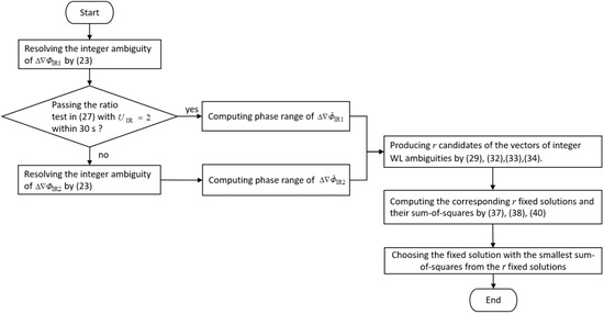
Figure 1.
The procedure of the modified phase-only method.
Once is obtained, we can remove the integer ambiguity from the IR combination to obtain the phase range as follows:
3.2.2. Candidates of Wide-Lane (WL) Integer Ambiguities
We use the EWL combinations and the phase ranges to determine integer EWL ambiguities. For s DD pairs, the linearized observation equation is expressed as:
where the observation vector is given as
and the parameter vector of DD integer EWL ambiguities is,
The symbol is the design matrix corresponding to . The symbol is the noise vector of . After the least-squares adjustment, we can obtain the vector of real-valued EWL ambiguities, . Then, the vector of integer EWL ambiguities, , is resolved by the LAMBDA method.
From Equations (23)–(31), the phase-only method neglects the DD ionospheric delays and resolve with a step-wise strategy. The similar strategy can be found in the typical TCAR method [10,31]. However, when the effect of DD ionospheric delay on is too large to be neglected, i.e., the effect is larger than half a cycle of , both the typical TCAR method and the phase-only method must find ways to eliminate the effect on . The typical TCAR method can be expanded with additional ionosphere parameters to eliminate the effect, e.g., the integrated TCAR method proposed in [19]; however, the phase-only method cannot use additional ionosphere parameters because of the absence of code measurements. As a result, potential candidates of are produced by a distance-dependent search range, as follows:
where R is a given size of the search region in integer cycles and N indicates the N-th entry in a vector. If there are s available satellites, then the number of candidates is . The size R is designed to compensate for the effects of ionospheric delays on the measurement , as used in Equation (30). The ionospheric delays vary dramatically with ionospheric conditions and ionosphere pierce points, and hence it is difficult to define a proper size of R to compensate for the delays. An upper bound of size R, which can guarantee that the correct is inside the search region, is pre-determined to overcome the problem. The upper bound is derived from the maximal DD ionospheric delay, denoted as , given as:
The maximal delay was produced by using simulation medium earth orbit (MEO) satellites and the IONosphere map EXchange format (IONEX) [32] of 29 October 2003, during which a solar storm occurred and the maximum vertical total electron content was about 250 TECU. Detailed information about can be found in [8]. The maximal delay can be given as a function of distance,
where L is the distance in kilometers.
We assume that r candidates of have been produced in the distance-dependent search range with the upper bound, and we can compute the candidates of the vectors of integer WL ambiguities. For , they are given as:
For , they are given as:
where the subscript .
3.2.3. Resolving Triple-Frequency DD Integer-Phase Ambiguities
Once the candidates of have been obtained, we resolve the triple-frequency DD integer phase ambiguities. We use the first candidate as a constraint to incorporate with the IF phase linear combination to resolve the first float solution, then use the second candidate to resolve the second float solution, and so on. In total, we can resolve r float solutions and these r linearized observation models are defined as:
with the constraint,
where the subscript , and the symbols and are the design matrices that correspond to vectors and , and the symbol H is the design matrix of the constraint vector.
After the least-squares adjustment, the r float solutions are computed as:
The biases and are caused by incorrect . For the r float solutions, the associated real-valued solutions of ambiguities, , are processed with the LAMBDA method to find the integer solutions of ambiguities, . Then, the r fixed solutions can be computed as:
Among the r fixed solutions, the solution with the smallest sum-of-squares is chosen, and its corresponding ratio test value is validated by using Equation (22). The detailed procedure for the determination of the phase range, candidates of WL integer ambiguities, and triple-frequency DD integer phase ambiguities is shown in Figure 1.
4. Experimental Analyses
The phase-only and phase-code methods were tested with BDS triple-frequency data. The results of the two methods were compared for ambiguity-resolution performance. The effect of code multipath on ambiguity resolution is discussed, and then the factors affecting the phase-only method and the success percentage of the two methods are elaborated.
The test baselines were 37 km and 256 km in length with stations located in a mid-low latitude region of southern Taiwan (longitude: 120–121°, latitude: 22–23°). The base station is situated on an open-sky rooftop. The unknown static stations were set up on roadsides, and hence their signals were influenced and reflected by surrounding buildings. The BDS triple-frequency measurements of the two baselines were collected using the Trimble NetR9 receivers under active ionospheric conditions near noon and afternoon. We used cutoff angles of 15° and 40° to represent normal and constrained environments, respectively. The number of available satellites over the two baselines is shown in Figure 2. The phase and code noises are represented by the difference of the IF linear combinations (DIF). Code DIF is represented as , and phase DIF is represented as after the integer ambiguities on and have been correctly removed. The DIF can eliminate the geometric term, ionospheric delay, and tropospheric delays, and thus it only reflects a weighted sum of triple-frequency DD noise [12]. We computed the DIF values of all DD pairs for all epochs over each baseline and then computed the root mean square (RMS) of the DIF values. Details of the two baselines are shown in Table 3. The strategy of handling measurement errors in the experiments is listed in Table 4. In this analysis, the true values of positioning results and integer ambiguity sets for the two baselines are obtained by static processing of the 2.5 h observation period.
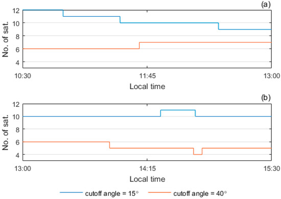
Figure 2.
Number of available satellites. (a) 37 km baseline; (b) 256 km baseline.
Table 3.
Information of the 37 km and 256 km test baselines.
Table 4.
Processing strategy for measurement errors.
After the distance-dependent errors, namely the DD atmospheric delays and orbital errors, are reduced by the processing strategy in Table 4, the number and distribution of visible satellites, i.e., satellite geometry, and measurement noises including multipath are the major factors affecting ambiguity resolution [36,37,38]. To reflect the influence of code noise on ambiguity resolution, we need to select some test sessions whose code noises are visibly different. Similarly, in order to understand the effects of phase noise and satellite geometry, we need to select some test sessions whose phase noises are different, and some test sessions whose satellite geometries are different. These sessions were chosen from the 2.5 h observation period, as listed in Table 5. For each session, the DIF values of all DD pairs for all epochs were computed and the related RMS value is listed in Table 5. In addition, we put the mean positional dilution of precision (PDOP) values in Table 5 to show the satellite geometry over these sessions. Sessions 1–5 refer to the 37 km baseline, and sessions 6–10 refer to the 256 km baseline.
Table 5.
Information of test sessions 1–10.
4.1. Effect of Code Multipath
To investigate the effect of code multipath on ambiguity resolution, in this section we processed sessions 1 and 2 with the phase-code and phase-only methods for the 37 km baseline since the two sessions had similar RMS of phase DIF, and similar mean PDOP, but different RMS of code DIF. For the same reason, we processed sessions 6 and 7 for the 256 km baseline. We smoothed out the random errors on the code DIF values of the four sessions with the Gaussian low-pass filter [39] to obtain the code multipath signals. The smoothed code multipath signals of the sessions 1and 2 are illustrated in Figure 3, and those of the sessions 6 and 7 are in Figure 4.
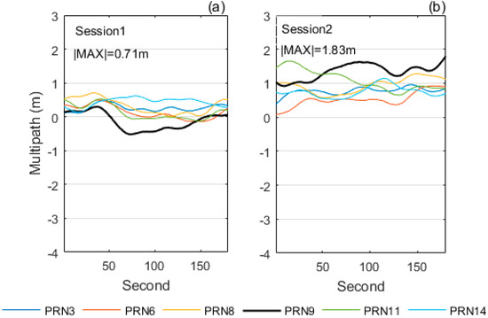
Figure 3.
Code multipath for sessions 1 and 2 over the 37 km baseline. The pivot satellite was PRN1, a geostationary satellite. (a) session 1; (b) session 2.
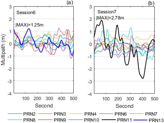
Figure 4.
Code multipath for sessions 6 and 7 over the 256 km baseline. The pivot satellite was PRN1, a geostationary satellite. (a) session 6; (b) session 7.
Figure 3 and Figure 4 reveal that the code multipath is present, as the smoothed code DIF values are visibly correlated in time. Furthermore, the maximum absolute value of the code multipath in session 2 is larger than that in session 1 over the 37 km baseline. Similarly, the maximum absolute value of the code multipath in session 7 is larger than that in session 6 over the 256 km baseline. We computed the time-to-first-fix (TTFF) for the above four sessions. The TTFF is the first epoch time that the accumulated ratio test value is larger than or equal to a given threshold, on the premise that the resolved integer ambiguities are the same as the true values of integer ambiguities.
The TTFF values of sessions 1, 2, 6, and 7 are listed in Table 6. Over the 37 km baseline, the phase-code method achieved the ambiguity resolution in 5 s in session 1 which had a smaller code multipath, and completed the ambiguity resolution in 96 s in session 2, whose code multipath was larger. In contrast, the phase-only method only needed 2 s to complete the ambiguity resolution in both sessions. Over the 256 km baseline, the phase-code method achieved the ambiguity resolution in 187 s in session 6 which had a smaller code multipath, and needed 342 s to complete the ambiguity resolution in session 7 whose code multipath was larger. On the other hand, the phase-only method only needed 109 s and 127 s in the two sessions, respectively. This shows that the phase-only method completes ambiguity resolution faster than the phase-code method, particularly when the code multipath is large.
Table 6.
Time-to-first-fix (TTFF) values at threshold U = 2 for sessions 1, 2, 6, and 7.
4.2. Effects of Phase Noise and Satellite Geometry
The factors affecting the phase-only ambiguity resolution are discussed in this section. Given that the phase-only method is free of code noise, we evaluated the effects of phase noise and satellite geometry. We processed sessions 3–5 for the 37 km baseline, and sessions 8–10 for the 256 km baseline with the phase-code and phase-only methods. The accumulated ratio test values of sessions 3–5 and of sessions 8–10 are shown in Figure 5 and Figure 6, respectively.
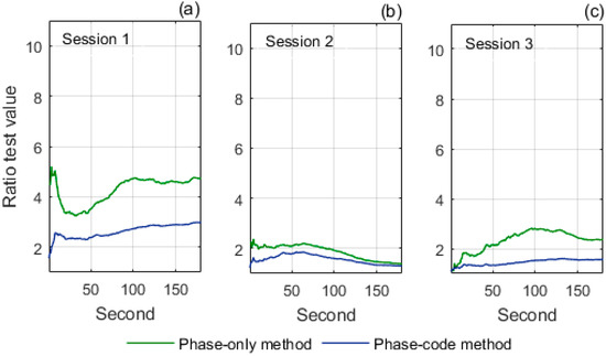
Figure 5.
Accumulated ratio test values of sessions 3, 4, and 5 over the 37 km baseline. (a) session 1; (b) session 2; (c) session 3.
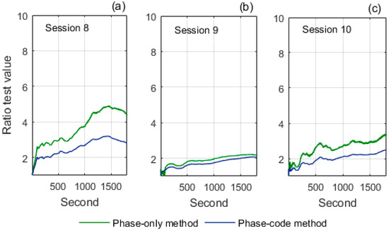
Figure 6.
Accumulated ratio test values of sessions 8, 9, and 10 over the 256 km baseline. (a) session 8; (b) session 9; (c) session 10.
For the results of the 37 km baseline in Figure 5, we can compare the accumulated ratio test values of session 3 with those of session 4 to investigate the effect of phase noise since the two sessions have different RMS of phase DIF but similar RMS of code DIF and mean PDOP. The comparison shows that the phase-only method generally produces higher ratio test values than the phase-code method, but the improvement in session 4 is less significant than in session 3. The reason is that the RMS of phase DIF in session 4 (0.006 m) is obviously larger than that in session 3 (0.004 m). This indicates that the improvement of the phase-only method is limited by large phase noise. We then compare the accumulated ratio test values of session 3 with session 5 to investigate the effect of satellite geometry since the two sessions have different mean PDOP but similar RMS of phase DIF and RMS of code DIF. The comparison shows that the improvement in ratio test values in session 5 is less significant than in session 3, as a result of the poorer mean PDOP in session 5 (3.2) than that in session 3 (2.4). This indicates that the improvement of the phase-only method is also impaired by poor satellite geometry.
In a similar way, for the results of the 256 km baseline in Figure 6, we can compare session 8 with session 9 to reflect the effect of phase noise, and compare session 8 with session 10 to reflect the effect of satellite geometry. The comparisons again indicate that the phase-only method generally produces higher ratio test values than the phase-code method, but the improvement is impaired by large phase noise and poor satellite geometry.
4.3. Success Percentage
In this section, we use success percentage to represent the performance of ambiguity resolution within a 3-min initialization time. The filter was initialized every 3 min and 50 test sessions were conducted during the whole 2.5 h observation period. Then, the success percentage was computed as follows:
where a successful test session has to achieve the TTFF.
Figure 7 displays the success percentages over the 37 km and 256 km baselines with commonly used ratio test thresholds (U = 2, 2.5, 3) [20,26]. Figure 7a,c show that the success percentages at cutoff angle = 15° (representing a normal environment) decrease noticeably when the threshold is increased from 2 to 3 for both methods. Figure 7b,d also show that the success percentages at cutoff angle = 40° (representing a constrained environment) decrease with increased thresholds for both methods. The reason is that, as previously stated, larger thresholds can avoid the ambiguity being incorrectly fixed but unnecessarily reject correctly fixed integer ambiguities. In all four figures, the phase-only method produces higher success percentages than the phase-code method with commonly used ratio test thresholds.
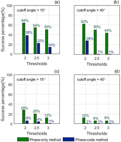
Figure 7.
Success percentages at thresholds U = 2, 2.5, 3. (a,b) 37 km; (c,d) 256 km.
5. A Demonstration in an Environment with Obvious Multipath Effects
In this section, we demonstrate the performance of the phase-only method in an environment with obvious multipath effects. We situated an unknown static station near reflective metal surfaces to collect BDS triple-frequency measurements contaminated by multipath. The surrounding environment of the unknown station is shown in Figure 8, where the metal surfaces are enclosed with red lines.
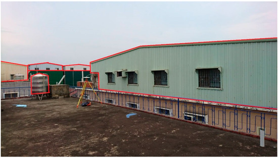
Figure 8.
Surrounding environment of the unknown station.
The experimental data was collected during 12:42–12:52 (local time) and the baseline length was 17 km. The smoothed code multipath signals are illustrated in Figure 9, where the maximum absolute value reaches 3.54 m.
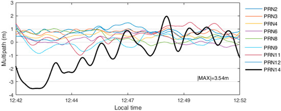
Figure 9.
Code multipath for the 17-km baseline. The pivot satellite was PRN1, a geostationary satellite.
At threshold U = 2, the TTFF value for the phase-code method is 466 s; while it is only 2 s for the phase-only method. The result shows that the phase-only method could be effective in improving ambiguity resolution when stations are situated in environments with apparent multipath effects.
6. Discussion
As demonstrated in the experimental analyses, the code multipath has a major impact on ambiguity resolution in conventional BDS phase-code methods. Because the code multipath on each satellite is dependent on the instantaneous geometric relation between the satellite, the receiver antenna, and the surrounding environment, it is very difficult (if not impossible) to handle rigorously by utilizing the commonly used code noise-weighting strategies, such as the elevation-dependent weighting function, the variance and covariance components estimation [40], and the related ray-tracing techniques [41,42]. In contrast, the proposed BDS phase-only method does not need to consider the weighting of code noise at all. That is to say, the phase-only method is able to achieve ambiguity resolution completely free of the influence of code multipath. What is more, in the future we can combine BDS with other triple-frequency code-division multiple access (CDMA) satellite navigation systems, such as GPS and Galileo, to further improve the phase-only ambiguity-resolution performance since better satellite geometry is critical to phase-only ambiguity resolution.
7. Conclusions
Conventional triple-frequency baseline computation accomplishes the ambiguity resolution with phase and code measurements. However, the computation is affected by the effect of multipath on the code measurements. To completely avoid code multipath, this study proposes a modified phase-only method for BDS ambiguity resolution. The phase-only method maneuvers two specific IR combinations to determine the phase range and uses this to replace the code measurement. Given that the phase-only method uses only BDS triple-frequency phase measurements, the effect of code noise, including code multipath, can be excluded fully.
The phase-only method is compared with a generalized phase-code method to evaluate the improvement in ambiguity resolution. Experimental results over medium and long baselines indicate that phase-only ambiguity resolution is feasible and generally produces a better performance, namely shorter TTFF and higher success percentages, than the phase-code ambiguity resolution. However, the improvement is subject to the phase noise and satellite geometry. A demonstration in an obvious multipath environment shows that the phase-only method could effectively reduce the TTFF from 466 s to 2 s.
Author Contributions
F.-Y.C. developed the method and completed all the tests, words, and diagrams. M.Y. proposed the research concept, completed the Discussion of this study, and was responsible for the manuscript. Both authors read and approved the final manuscript.
Funding
This research was funded by Ministry of Science and Technology of Taiwan. Grant No. 104-2221-E-006-047-MY3, No. 105-2119-M-006-027, and No. 106-2119-M-006-019.
Acknowledgments
The authors are indebted to the Ministry of Science and Technology of Taiwan for its support.
Conflicts of Interest
The authors declare no conflict of interest.
References
- Kleusberg, A. Kinematic relative positioning using GPS code and carrier beat phase observations. Mar. Geodesy 1986, 10, 257–274. [Google Scholar] [CrossRef]
- Bossler, J.D.; Goad, C.C.; Bender, P.L. Using the global positioning system (GPS) for geodetic positioning. Bull. Géodesique 1980, 54, 553–563. [Google Scholar] [CrossRef]
- Goad, C.C.; Remondi, B.W. Initial relative positioning results using the global positioning system. Bull. Géodesique 1984, 58, 193–210. [Google Scholar] [CrossRef]
- Teunissen, P.J.G.; de Jonge, P.J.; Tiberius, C.C.J.M. The least-squares ambiguity decorrelation adjustment: Its performance on short GPS baselines and short observation spans. J. Geodesy 1997, 71, 589–602. [Google Scholar] [CrossRef]
- Odijk, D. Ionosphere-free phase combinations for modernized GPS. J. Surv. Eng. 2003, 129, 165–173. [Google Scholar] [CrossRef]
- Kleusberg, A.; Teunissen, P.J.G. GPS for Geodesy; Springer: Berlin, Germany, 1996. [Google Scholar]
- Teunissen, P.J.G.; Odijk, D. Rank-defect integer estimation and phase-only modernized GPS ambiguity resolution. J. Geodesy 2003, 76, 523–535. [Google Scholar] [CrossRef]
- Chu, F.-Y.; Yang, M.; Wu, J. A new approach to modernized GPS phase-only ambiguity resolution over long baselines. J. Geodesy 2016, 90, 241–254. [Google Scholar] [CrossRef]
- Cocard, M.; Bourgon, S.; Kamali, O.; Collins, P. A systematic investigation of optimal carrier-phase combinations for modernized triple-frequency GPS. J. Geodesy 2008, 82, 555–564. [Google Scholar] [CrossRef]
- Feng, Y. GNSS three carrier ambiguity resolution using ionosphere-reduced virtual signals. J. Geodesy 2008, 82, 847–862. [Google Scholar] [CrossRef]
- Chen, H.-C.; Huang, Y.-S.; Chiang, K.-W.; Yang, M.; Rau, R.-J. The performance comparison between GPS and BeiDou-2/COMPASS: A perspective from Asia. J. Chin Inst. Eng. 2009, 32, 679–689. [Google Scholar] [CrossRef]
- Montenbruck, O.; Hauschild, A.; Steigenberger, P.; Hugentobler, U.; Teunissen, P.; Nakamura, S. Initial assessment of the COMPASS/BeiDou-2 regional navigation satellite system. GPS Solut. 2013, 17, 211–222. [Google Scholar] [CrossRef]
- CSNO. BeiDou Navigation Satellite System Signal in Space Interface Control Document: Open Service Signal, Version 2.0. China Satellite Navigation Office, December 2013. Available online: http://www.beidou.gov.cn (accessed on 1 June 2016).
- Tang, W.; Deng, C.; Shi, C.; Liu, J. Triple-frequency carrier ambiguity resolution for BeiDou navigation satellite system. GPS Géodesique 2014, 18, 335–344. [Google Scholar] [CrossRef]
- Zhao, Q.; Dai, Z.; Hu, Z.; Sun, B.; Shi, C.; Liu, J. Three-carrier ambiguity resolution using the modified TCAR method. GPS Solut. 2014, 19, 589–599. [Google Scholar] [CrossRef]
- Zhang, X.; He, X. Performance analysis of triple-frequency ambiguity resolution with BeiDou observations. GPS Solut. 2015, 20, 269–281. [Google Scholar] [CrossRef]
- He, X.; Zhang, X.; Tang, L.; Liu, W. Instantaneous real-time kinematic decimeter-level positioning with BeiDou triple-frequency signals over medium baselines. Sensors 2016, 16, 1. [Google Scholar] [CrossRef] [PubMed]
- Li, B.; Feng, Y.; Gao, W.; Li, Z. Real-time kinematic positioning over long baselines using triple-frequency BeiDou signals. IEEE Trans. Aerosp. Electron. Syst. 2016, 51, 3254–3269. [Google Scholar] [CrossRef]
- Leick, A.; Rapoport, L.; Tatarnikov, D. GPS Satellite Surveying, 4th ed.; John Wiley & Sons, Inc.: Hoboken, NJ, USA, 2015. [Google Scholar]
- Zhang, X.; He, X. BDS triple-frequency carrier-phase linear combination and their characteristics. Sci. China Earth Sci. 2015, 58, 896–905. [Google Scholar] [CrossRef]
- Hatch, R. The Synergism of GPS Code and Carrier Measurement. In Proceedings of the Third International Geodetic Symposium on Satellite Doppler Positioning, Las Cruces, NM, USA, 8–12 February 1982. [Google Scholar]
- Niell, A.E. Global mapping functions for the atmosphere delay at radio wavelengths. J. Geophys. Res. 1996, 101, 1978–2012. [Google Scholar] [CrossRef]
- Teunissen, P.J.G. The least-squares ambiguity decorrelation adjustment: A method for fast GPS integer ambiguity estimation. J. Geodesy 1995, 70, 65–82. [Google Scholar] [CrossRef]
- Euler, H.J.; Schaffrin, B. On a Measure for the Discernibility between Different Ambiguity Solutions in the Static-kinematic GPS-mode. In Proceedings of the IAG Symposia, Banff, AL, Canada, 10–13 September 1990. [Google Scholar]
- Verhagen, S. Integer ambiguity validation: An open problem? GPS Solut. 2004, 8, 36–43. [Google Scholar] [CrossRef]
- Verhagen, S.; Teunissen, P.J.G. The ratio test for future GNSS ambiguity resolution. GPS Solut. 2013, 17, 535–548. [Google Scholar] [CrossRef]
- Kalman, R.E. A new approach to linear filtering and prediction problems. J. Basic Eng. 1960, 82, 35–45. [Google Scholar] [CrossRef]
- Hopfield, H.S. Two-quartic tropospheric refractivity profile for correcting satellite data. J. Geophys. Res. 1969, 74, 4487–4499. [Google Scholar] [CrossRef]
- Goad, C.; Yang, M. A new approach to precision airborne GPS positioning for photogrammetry. Photogramm. Eng. Remote Sens. 1997, 63, 1067–1077. [Google Scholar]
- Feng, Y.; Li, B. Three carrier ambiguity resolutions: Generalised problems, models and solutions. J. Glob. Position. Syst. 2009, 8, 115–123. [Google Scholar] [CrossRef]
- Vollath, U.; Birnbach, S.; Landau, H. Analysis of Three-carrier Ambiguity Resolution (TCAR) Technique for Precise Relative Positioning in GNSS-2. In Proceedings of the ION GPS-98, Nashville, TN, USA, 15–18 September 1998. [Google Scholar]
- Schaer, S.; Gurtner, W.; Feltens, J. The Ionosphere Map Exchange Format Version 1. In Proceedings of the IGS Analysis Centers Workshop, Darmstadt, Germany, 9–11 February 1998. [Google Scholar]
- Montenbruck, O.; Steigenberger, P.; Prange, L.; Deng, Z.; Zhao, Q.; Perosanz, F.; Romero, I.; Noll, C.; Sturze, A.; Weber, G.; et al. The Multi-GNSS experiment (MGEX) of the International GNSS Service (IGS)—achievements, prospects and challenges. Adv. Space Res. 2017, 59, 1671–1691. [Google Scholar] [CrossRef]
- Nadarajah, N.; Teunissen, P.J.G.; Sleewaegen, J.-M.; Montenbruck, O. The mixed-receiver BeiDou inter-satellite-type bias and its impact on RTK positioning. GPS Solut. 2015, 19, 357–368. [Google Scholar] [CrossRef]
- Hofmann-Wellenhof, B.; Lichtenegger, H.; Wasle, E. GNSS—Global Navigation Satellite Systems; SpringerWienNewYork: Wien, Austria, 2008. [Google Scholar]
- Ji, S.; Chen, W.; Zhao, C.; Ding, X.; Chen, Y. Single epoch ambiguity resolution for Galileo with the CAR and LAMBDA methods. GPS Solut. 2007, 11, 259–268. [Google Scholar] [CrossRef]
- Chu, F.-Y.; Yang, M. GPS/Galileo long baseline computation: Method and performance analyses. GPS Solut. 2014, 18, 263–272. [Google Scholar] [CrossRef]
- Odolinski, R.; Teunissen, P.J.G.; Odijk, D. Combined BDS, Galileo, QZSS and GPS single-frequency RTK. GPS Solut. 2015, 19, 151–163. [Google Scholar] [CrossRef]
- Gonzalez, R.C.; Woods, R.E. Digital Image Processing, 3rd ed.; Pearson Education: London, UK, 2017. [Google Scholar]
- Koch, K.R. Parameter Estimation and Hypothesis Testing in Linear Models, 2nd ed.; Springer: Berlin, Germany, 1999. [Google Scholar]
- Hsu, L.-T.; Tokura, H.; Kubo, N.; Gu, Y.; Kamijo, S. Multiple faulty GNSS measurement exclusion based on consistency check in urban canyons. IEEE Sens. J. 2017, 17, 1558–1748. [Google Scholar] [CrossRef]
- Lau, L.; Cross, P. Development and testing of a new ray-tracing approach to GNSS carrier-phase multipath modelling. J. Geodesy 2007, 81, 713–732. [Google Scholar] [CrossRef]
© 2018 by the authors. Licensee MDPI, Basel, Switzerland. This article is an open access article distributed under the terms and conditions of the Creative Commons Attribution (CC BY) license (http://creativecommons.org/licenses/by/4.0/).