Article

A Framelet-Based Iterative Pan-Sharpening Approach

School of Mathematical Sciences, University of Electronic Science and Technology of China, Chengdu 611731, Sichuan, China
*
Authors to whom correspondence should be addressed.
Remote Sens. 2018, 10(4), 622; https://doi.org/10.3390/rs10040622
Submission received: 7 March 2018 / Revised: 12 April 2018 / Accepted: 16 April 2018 / Published: 18 April 2018
(This article belongs to the Section Remote Sensing Image Processing)

Abstract

:
Pan-sharpening is used to fuse multispectral images and panchromatic images to produce a multispectral image with high spatial resolution. In this paper, we design a new iterative method based on framelet for pan-sharpening. The proposed model takes advantage of the upsampled multispectral image and a linear relation between the panchromatic image and the latent high-resolution multispectral image. Since the sparsity of the pan-sharpened image under a B-spline framelet transform is assumed, we regularize the model by penalizing l 1 norm of a framelet based term. The model is solved by a designed algorithm based on alternating direction method of multipliers (ADMM). For better performance, we propose an iterative strategy to pick up more spectral and spatial details. Experiments on four datasets demonstrate that the proposed method outperforms several existing pan-sharpening methods.

Graphical Abstract

1. Introduction

An optical satellite usually acquires two images describing the same scene almost simultaneously, which are called multispectral (MS) image and panchromatic (PAN) image respectively. The former is a multichannel image with low spatial resolution, while the latter is a single channel image with rich spatial details. Despite the fact that MS image can be of over eight bands and the resolution of PAN image can be less than half a meter, their superiority cannot be synthesized in one image due to physical and technological constraints. However, pan-sharpening techniques are capable of creating a multichannel image with high spatial resolution out of these two images, which is of great importance for remote sensing. More specifically, pan-sharpening plays an important role in the interpretation of remote sensing scenes and can be used as a preliminary step of various remote sensing tasks such as object recognition [1], change detection [2] and so on. Therefore, these techniques attract much attention of scientific community.
Among various pan-sharpening methods having been proposed in the literature, many of them can be put into two main categories: component substitution (CS) and multiresolution analysis (MRA). CS mainly involves three steps: firstly a spectral transformation of MS image, then a replacement of its spatial component with PAN image, and finally an inverse transformation. This class includes classical methods such as intensity-hue-saturation (IHS) [3], principal component analysis (PCA) [4], Gram-Schmidt spectral sharpening (GS) [5] and recent methods based on mean information [6] and image matting model [7]. As for MRA, it focuses on an injection process in which spatial details extracted from PAN image are added to upsampled MS image. Examples of this class include wavelet transform based methods [8,9,10], Laplacian Pyramid based methods [11], and methods based on other transforms [12,13].
Different from the two categories mentioned above, there are also other types of pan-sharpening methods. This family includes those based on Bayesian paradigm [14], total variation [15,16], gradient operator [17,18], sparse representation [19], super-resolution techniques [20], convolution neural network [21] and so on. Recently, Deng et al. [22] propose a novel variational model for pan-sharpening in which intensity function of the unknown image is considered from a continuous point of view. The related continuous function is made up of two components. Assumption is made that the former lies in a Reproducing Kernel Hilbert Space (RKHS) while the latter can be approximated by linear combination of approximated Heaviside functions (AHF). This model outperforms several state-of-the-art pan-sharpening methods according to experiments on two datasets. However, its good performance relies on a large amount of computation, which results in rather long running time.
In this paper, a new iterative algorithm for pan-sharpening is proposed as an attempt to simplify RKHS method. We make use of the information from MS image by generating its upsampled form. The linear relation [22,23] between PAN image and bands of the image to be estimated is also considered in the model. A framelet based term is introduced as regularization. Besides, we adopt an iterative strategy similar to [22] to improve performance of the algorithm. The framework of the proposed approach can be seen in Figure 1. By utilizing real data from Pléiades, Quickbird, WorldView-2 and SPOT-6, we compare several existing pan-sharpening methods with the proposed method. These results show spatial and spectral fidelity of the proposed method. Meanwhile, they confirm a much less running time than RKHS method, suggesting that framelet based regularization is more mature and easier to compute.
The rest of this paper is arranged as follows. Section 2 reviews the related work [22]. Then in Section 3 the new iterative algorithm is presented. Section 4 is a display of visual and numerical experimental results together with some discussions about the proposed method. Finally, conclusion is drawn in Section 5.

2. Related Work

To begin with, we introduce several notations to be used throughout this paper. Let MS R m 1 × n 1 × T be the original multispectral image with T bands, each band denoted as MS i R m 1 × n 1 . Let MS ˜ R m 2 × n 2 × T be the upsampled multispectral image, each band denoted as MS i ˜ R m 2 × n 2 . MS ^ represents the high-resolution multispectral image to be estimated, with MS i ^ R m 2 × n 2 being the ith band of it. Moreover, the original panchromatic image is P R m 2 × n 2 .
Deng et al. propose a new iterative pan-sharpening algorithm [22], which is an extension of their previous work on super-resolution [24]. They view the pan-sharpening problem as an intensity estimation process for the unknown image MS ^ . The intensity of MS ^ is modelled as a hidden continuous function. It consists of two different components, a smooth one and a non-smooth one. The former is assumed to be an element of a special function space called Reproducible Kernel Hilbert Space (RKHS), while the latter is formulated as a linear combination of approximated Heaviside functions (AHF).
Specifically, let f i , i = 1 , 2 , , T , be the underlying continuous intensity function corresponding to the ith band of MS ^ . Without loss of generation, the domain is restricted such that z = ( x , y ) [ 0 , 1 ] × [ 0 , 1 ] . The smooth component is expressed as ν = 1 M d ν , i ϕ ν , i ( z ) + s = 1 n c s , i ξ s , i ( z ) . These two series lie in two different RKHS, with ϕ ν , i ( z ) , ν = 1 , 2 , , M , and ξ s , i ( z ) , s = 1 , 2 , , n , being basis functions in each RKHS respectively. d ν , i , ν = 1 , 2 , , M , together with c s , i , s = 1 , 2 , , n , are the corresponding coefficients. As for the non-smooth component, a family of Heaviside functions is considered to implement the approximation. However, since Heaviside functions are singular at the origin, which makes differentiation impossible to be taken there, they are approximated by a smooth form, i.e., approximated Heaviside functions (AHF). In 2D case, this smooth alternative takes the form of ψ ( ( c o s θ j , i , s i n θ j , i ) · z + c ρ , i ) , actually representing an edge with θ elevation at a location specified by c ρ , i . It is a generalization of the 1D form ψ ( x ) = 1 2 + 1 π a r c t a n ( x ξ ) , where ξ is a positive parameter to control smoothness. Therefore, f i , i = 1 , 2 , , T , is finally modelled as:
f i = ν = 1 M d ν , i ϕ ν , i ( z ) + s = 1 n c s , i ξ s , i ( z ) + j = 1 k ρ = 1 n ω j , i ψ ( ( c o s θ j , i , s i n θ j , i ) · z + c ρ , i ) .
For more details, see [22,24].
By evaluating on a fine grid, (1) can be discretized so that it becomes a form involving simple matrix multiplication. Let T h R m 2 n 2 × M , K h R m 2 n 2 × m 2 n 2 and Ψ h R m 2 n 2 × m ( m = k · n ) denote matrices whose entries are generated by evaluating ϕ ν , i ( z ) , ξ s , i ( z ) , and ψ ( ( c o s θ j , i , s i n θ j , i ) · z + c ρ , i ) on a fine grid. Then each band of the desired multichannel image with high spatial resolution can be computed as follows:
MS i ^ = T h d i + K h c i + Ψ h β i , i = 1 , 2 , , T .
Hence the pan-sharpening problem is converted into a problem of coefficient estimation. In [22], the coefficients are computed by minimizing the following model:
min d i , c i , β i 1 N i = 1 T T h d i + K h c i + Ψ h β i MS i ˜ 2 2 + μ 2 i = 1 T c i T K l c i + λ 1 2 i = 1 T β i 1 + λ 2 2 i = 1 T ω i ( T h d i + K h c i + Ψ h β i ) P 2 2 ,
where N is the number of pixels that MS ^ contains. μ , λ 1 , and λ 2 are positive parameters. MS i ˜ is generated by an upsampling process via GS method [5]. K l R m 1 n 1 × m 1 n 1 is a coarser version of K h , i.e., the discretization process is done on a coarser grid. ω i are weights reflecting the contribution of each band of MS ^ to the linear combination which approximates the panchromatic image P. This linear approximation and its variants are assumed by many methods, e.g., [23,25].
After the coefficients d i , c i , β i are obtained, the high-resolution multispectral image can be computed by (2). Furthermore, model (3) is combined with an iterative strategy. It will be detailed in Section 3 since it is used in the method proposed in this paper as well.

3. The Proposed Method

Empirical results in [22] show that RKHS method outperforms several state-of-the-art pan-sharpening methods both in the perspective of spatial and spectral fidelity. However, the RKHS based model of MS ^ is quite complicated, since it is not easy to implement in actual calculation. In addition, the regularization terms of (3) involve not only l 1 norm of β i but also quadratic function of c i (both summed by band), which adds to computational burden. As a result, the algorithm is rather time consuming. Therefore, it is natural to raise a question. Can we simplify model (3) without loss of its advantage, i.e., high-level spatial and spectral performance? A possible way is not to make efforts to build a complicated model of MS ^ , but seek for another technique of regularization instead. This is exactly why we turn to framelet.
Piecewise smooth functions, for instance images, can be sparsely approximated by framelet system efficiently [26]. As a result, framelet techniques are used in literature to address the problems like image restoration (e.g., [26,27,28]). Recently, it is also applied to pan-sharpening. For instance, a framelet based MRA scheme is considered in [29]. A variational model [30] based on assumptions related to framelet coefficients, geometry keeping, spectral preserving and the sparsity of the image in the framelet domain is also proposed. They are able to obtain good results. Nevertheless, in this section, we consider a combination of variational model and iterative strategy instead of building a complicated model, i.e., we try to build a simple framelet based variational model and then combine it with an iterative strategy to yield a novel and effective approach for pan-sharpening.
In discrete case, let W and W T denote fast framelet decomposition and construction respectively. They are constructed by unitary extension principle (UEP) [31], and satisfy the relation W T W = I . In this paper, we use the piecewise linear B-spline framelets [26]. An L-level framelet transform of an image u [26] can be denoted as:
W u = { W l , j u , 0 l L 1 , j I } ,
where W l , j u denotes the coefficients of u in framelet band j at level l under the framelet transform, and I is the index set of all framelet bands. Throughout this paper, we empirically set L = 1 . For more theoretical details of framelet, see e.g., [32].
Consequently, by employing framelet based regularization, (3) can be modified. Each band of MS ^ is computed by minimizing the following function:
min MS i ^ 1 2 i = 1 T MS i ^ MS i ˜ 2 2 + α 2 i = 1 T ω i MS i ^ P 2 2 + i = 1 T λ i · W ( MS i ^ ) 1 ,
where α and λ i are parameters. Dot product is used in the third term since there are more than one framelet band, as (4) suggested. Coefficients for bands of MS ^ , i.e., ω i , are estimated automatically by a linear regression [23] between the original multispectral image and downsampled panchromatic image. The upsampled multispectral image MS i ˜ is generated via GS method. Note that this model can also be viewed as an extension of the so-called analysis based model for image restoration (e.g., [33,34]). Each l 1 term of (5) is in accordance with that defined in the analysis based model. Concretely, it can be expressed as
λ i · W ( MS i ^ ) 1 = j I λ i , j | W i , j ( MS i ^ ) | 1 .
This expression is the case where 1-level framelet transform is imposed on MS i ^ , as we emphasized above.
Model (5) can be solved by methods such as primal-dual method [35] and ADMM [36] efficiently. We choose ADMM here, whose application covers a wide range of image processing, such as image denoising [37], image super-resolution [38], tensor completion [39], image destriping [40,41] and so on. Its convergence is guaranteed by many works such as [42,43]. Due to non-smoothness caused by l 1 term, the first step is to rewrite (5) as an equivalent form through substitution of variables:
min u i , V i , MS i ^ 1 2 i = 1 T MS i ^ MS i ˜ 2 2 + α 2 i = 1 T ω i V i P 2 2 + i = 1 T λ i · u i 1 s . t . , u i = W ( MS i ^ ) , V i = MS i ^ , i = 1 , , T .
Then we can obtain the augmented Lagrangian of (7), i.e.,
L ( MS i ^ , u i , V i , D i , E i ) = 1 2 i = 1 T MS i ^ MS i ˜ 2 2 + α 2 i = 1 T ω i V i P 2 2 + i = 1 T λ i · u i 1 + β 2 2 i = 1 T u i W ( MS i ^ ) 2 2 + i = 1 T E i T ( u i W ( MS i ^ ) ) + β 1 2 i = 1 T V i MS i ^ 2 2 + i = 1 T D i T ( V i MS i ^ ) ,
where D i and E i are Lagrangian multipliers, β 1 and β 2 are two positive parameters.
Now we denote F i = D i / β 1 and G i = E i / β 2 . According to ADMM, problem (7) can be solved by implementing the following iterative scheme:
(1)
For i = 1 , , T , update each u i ( k ) by solving:
u i ( k + 1 ) = arg min u i λ i · u i 1 + β 2 2 u i W ( MS i ^ ( k ) ) + G i ( k ) 2 2 .
(2)
For i = 1 , , T , update each V i ( k ) by solving:
V i ( k + 1 ) = arg min V i α 2 1 j < i ω j V j ( k + 1 ) + ω i V i + i < j T ω j V j ( k ) P 2 2 + β 1 2 V i MS i ^ ( k ) + F i ( k ) 2 2 .
(3)
For i = 1 , , T , update each MS i ^ ( k ) by solving:
MS i ^ ( k + 1 ) = arg min MS i ^ 1 2 MS i ^ MS i ˜ 2 2 + β 1 2 V i ( k + 1 ) MS i ^ + F i ( k ) 2 2 + β 2 2 u i ( k + 1 ) W ( MS i ^ ) + G i ( k ) 2 2 .
(4)
For i = 1 , , T , update each F i ( k ) by F i ( k + 1 ) = F i ( k ) + ( V i ( k + 1 ) MS i ^ ( k + 1 ) ) .
(5)
For i = 1 , , T , update each G i ( k ) by G i ( k + 1 ) = G i ( k ) + ( u i ( k + 1 ) W ( MS i ^ ( k + 1 ) ) .
Note that (9)–(11) have closed-form solutions. Using soft-thresholding operator (e.g., [44]) T τ , u i ( k + 1 ) can be rewritten as:
u i ( k + 1 ) = T λ i / β 2 ( W ( MS i ^ ( k ) ) G i ( k ) ) ,
where T τ ( ν ) is defined entry-wise by
T τ ( ν ) = ν | ν | max { | ν | τ , 0 } ,
As for (10) and (11), they can be solved easily as follows:
V i ( k + 1 ) = α ω i ( P 1 j < i ω j V j ( k + 1 ) i < j T ω j V j ( k ) ) + β 1 ( MS i ^ ( k ) F i ( k ) ) α ω i 2 + β 1 ,
MS i ^ ( k + 1 ) = MS i ˜ + β 1 ( V i ( k + 1 ) + F i ( k ) ) + β 2 W T ( u i ( k + 1 ) + G i ( k ) ) β 1 + β 2 + 1 .
In order to facilitate illustration of the proposed algorithm, we summarize these steps of ADMM as Algorithm 1. Note that for simplicity of form, we write each iteration of ADMM in Algorithm 1 in an order slightly different from what we mentioned above, but it is easy to validate that they give the same results.
Algorithm 1 ADMM scheme for the proposed model
 Input: panchromatic image P , upsampled multispectral image MS ˜ , ω i α , λ i , β 1 , β 2 .
 Output: high-resolution multispectral image MS ^ .
  while not converged do
   for i = 1 : T do
    (1) Solve u i ( k + 1 ) by (12).
    (2) Solve V i ( k + 1 ) by (14).
    (3) Solve MS i ^ ( k + 1 ) by (15).
    (4) Update F i ( k ) by F i ( k + 1 ) = F i ( k ) + ( V i ( k + 1 ) MS i ^ ( k + 1 ) ) .
    (5) Update G i ( k ) by G i ( k + 1 ) = G i ( k ) + ( u i ( k + 1 ) W ( MS i ^ ( k + 1 ) ) ) .
   end for
  end while
Although Algorithm 1 itself is a complete algorithm, there is still room for improvement. Thus an iterative stategy is considered. For accordance of notations, let P ( 1 ) = P and MS ( 1 ) = MS . Similarly, denote the first output of Algorithm 1 as I ( 1 ) . After obtaining MS ^ , we compute P ( 2 ) = P i = 1 T ω i MS i ^ . In addition, let MS ˜ ( 2 ) = U ( MS - D ( MS ^ ) ) . D represents a downsampling operator, and U represents the upsampling process by which MS ˜ is generated. Now we view P ( 2 ) and MS ˜ ( 2 ) as new inputs for Algorithm 1 instead of the original P and MS ˜ . The resulting new output can be denoted as I ( 2 ) . By repeating this strategy, we obtain a series of I ( j ) , j = 2 , 3 , , γ . Then the sum of all I ( j ) , j = 1 , 2 , , γ , is taken as the final high-resolution multichannel image. This iterative strategy is adopted in not only pan-sharpening [22] but also image super-resolution [24].
Now we can summarize the procedures above as Algorithm 2:
Algorithm 2 The proposed iterative pan-sharpening algorithm
 Input: panchromatic image P , multispectral image MS , ω i α , λ i , β 1 , β 2 .
 Output: high-resolution multispectral image MS ^ .
  1. Initialization: MS ( 1 ) = MS , P ( 1 ) = P .
  for j = 1 : γ do
    (1) Upsample MS ( j ) to obtain MS ˜ ( j ) .
    (2) Compute I ( j ) by implementing Algorithm 1 ( MS ˜ ( j ) , P ( j ) instead of MS ˜ , P as input).
    (3) Update P ( j ) by P ( j + 1 ) = P ( j ) i = 1 T ω i I i ( j ) .
    (4) Update MS ( j ) by MS ( j + 1 ) = MS ( j ) D ( I ( j ) ) .
  end for
  2. Compute the final output: MS ^ = j = 1 γ I ( j ) .
Note that γ is the number of outer iterations. The downsampling process D in each iteration is completed through a combination of two steps: compute the modulation transfer function of I ( j ) with Gaussian filter and then interpolate it to the size of MS in a “nearest” way [22]. And the upsampling process is done by GS method.

4. Results and Discussion

In this section, we firstly utilize four datasets to compare the proposed method with several pan-sharpening methods. After that, discussions related to the number of outer iterations of Algorithm 2 are discussed. Results on time cost are presented as well.
The tested datasets are acquired by Quickbird (4 bands, 512 × 512 ), Pléiades (4 bands, 1024 × 1024 ), WorldView-2 (4 bands, 800 × 800 ), and SPOT-6 (4 bands, 1024 × 1024 ). The dataset of Quickbird can be downloaded from http://glcf.umd.edu/data/quickbird/chilika.shtml. And the dataset of Pléiades is downloaded together with the source codes of [45] from http://openremotesensing.net/knowledgebase/quality-assessment-of-pan-sharpening-methods-in-high-resolution-satellite-images-using-radiometric-and-geometric-index/. As for datasets of WorldView-2 and SPOT-6, we downloaded them from http://cms.mapmart.com/Samples.aspx.
Since high resolution multispectral images are not available in the datasets, we follow Wald’s protocol [46]. Therefore, the original multispectral images in the datasets are treated as ground truth. The scale ratio is 4, thus the simulated low-resolution multispectral images (4 bands) are of the size 128 × 128 , 256 × 256 , 200 × 200 , and 256 × 256 respectively. Each of them is downsampled from the corresponding ground truth in the same way as that in Algorithm 2, i.e., filter the ground truth by a Gaussian filter matched with the modulation transfer function (MTF) and then downscale it by “nearest” interpolation. As for each P , it is generated by combining bands of the ground truth linearly.
Parameters of the proposed algorithm are empirically set as follows. We use 1-level piecewise linear B-spline framelet. For each band, λ i is equally set as:
λ i = 10 4 0 1 1 1 1 1 1 1 1 .
Other model parameters in (8) are set as α = 1.5 , β 1 = 0.5 , and β 2 = 0.5 , with coefficients ω i estimated by linear regression. In addition, the number of the external iterations in Algorithm 2, i.e., γ , is set as 5. For different datasets, these settings may not always be the best choice, but we unify them to display stability of the proposed method and also to save efforts of tuning.
Methods compared with the proposed method comprise some classical pan-sharpening methods (PCA [4], GS [5], high-pass filtering (HPF) [47], and modulation transfer function-generalized Laplacian Pyramid (MTFGLP) [48,49]) and different kinds of recent state-of-the-art methods (pan-sharpening with hyper-Laplacian prior (PHLP) [50], nonlinear intensity-hue-saturation (NIHS) [51], and RKHS [22]). All the experiments are conducted in MATLAB on a laptap with 4GB RAM and 1.70 GHz Intel(R) Core(TM) i5-4210U CPU.

4.1. Visual Comparison

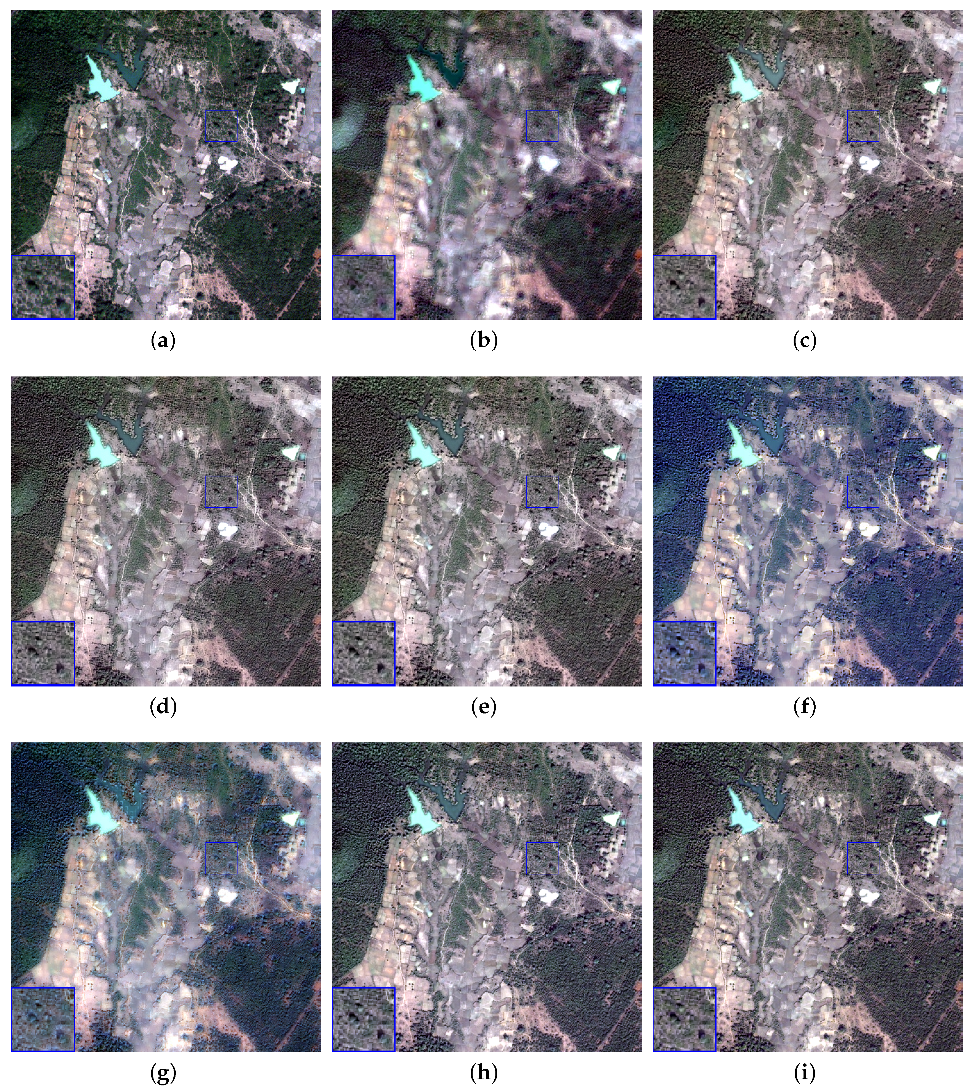
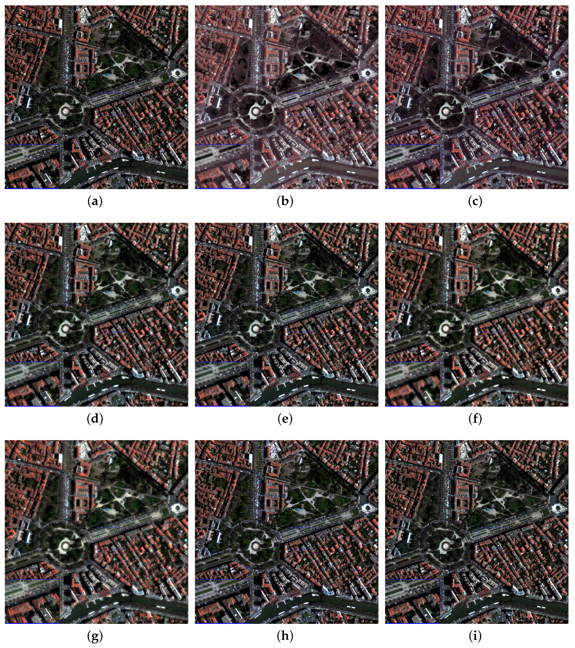
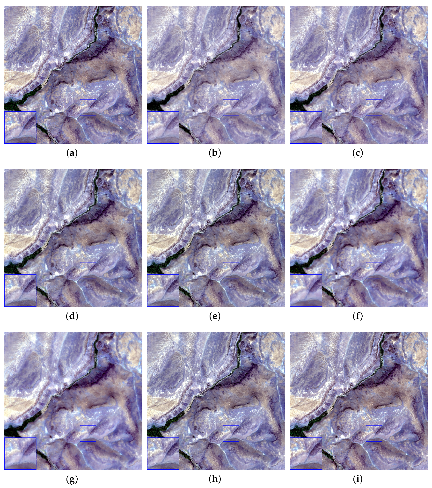
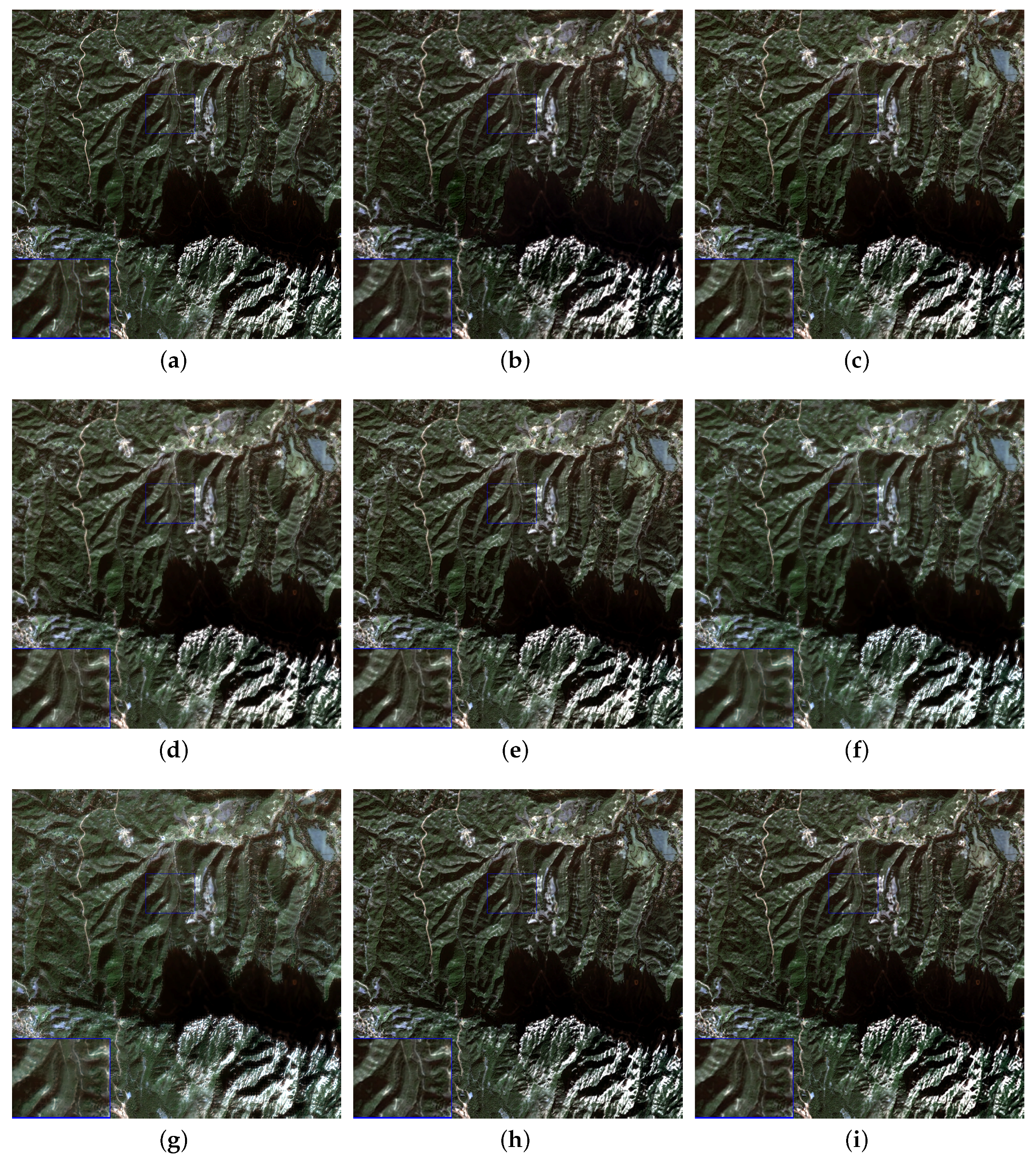
Figure 2, Figure 3, Figure 4 and Figure 5 show visual results obtained by conducting experiments on four datasets aforementioned. Each set of figures contains output images produced by eight different methods. Each ground truth is also presented as reference. For better visualization, we show local enlarged images at the bottom-left corner of each output image.
It is obvious that all of the other methods perform better than PCA method both in terms of spatial quality and spectral fidelity according to Figure 2, Figure 3 and Figure 4. GS method outperforms PCA method significantly but generally fails to avoid great spectral distortion, which is most visible on Quickbird dataset and Pléiades dataset. NIHS method and PHLP method preserve spectral characteristics quite well. However, from the perspective of spatial details, they tend to generate excessive smooth results, thus the pan-sharpened images provided by them lack much sharp spatial information compared with the reference images.
HPF method and MTFGLP method are visually without much spectral distortion and are able to keep more spatial details. However, a closer look at their resulting images, e.g., in Figure 3, suggests that they are not able to provide as many spatial details as the proposed method does. Finally, it is noticeable that RKHS method and the proposed method achieve the best visual performance on the last three experimented datasets. Actually, visual comparisons show little disparity for these four methods. However, we will demonstrate that the proposed method gives the best quantitative results in Section 4.2.

4.2. Quantitative Comparison

Several quantitative indices are employed to report the performance of different pan-sharpening methods. To evaluate spectral distortion, we use spectral angle mapper (SAM) [52], erreur relative globale adimensionnelle de synthése (ERGAS) [52], universal image quality index (Q) [53] together with its vector extension Q4 [54], and relative average spectral error (RASE) [55] (the larger Q and Q4 and the smaller SAM and ERGAS, the better performance). Correlation coefficient (CC) [56], with 1 being its ideal value, acts as spatial quality metric. Meanwhile, we use peak signal-to-noise ratio (PSNR) and root mean square error (RMSE) as metrics of fusion accuracy. Generally speaking, better performance is achieved when PSNR is larger and RMSE is smaller.
In each experiment, most of the compared methods require an upsampled multispectral image as an input. Unless specially specified in the literature, we unifiedly generate them by interpolating via a kernel function which is a polynomial with 23 coefficients [57].
The quantitative results of four datasets with regard to eight metrics are reported in Table 1, Table 2, Table 3 and Table 4. They clearly validate that the rest of the methods outperform PCA method as visual comparison in Section 4.1 preliminarily confirmed. GS method maintain spectral fidelity well on Quickbird dataset and WorldView-2 dataset, while on the rest two datasets it performs not so well. Compared with methods such as MTFGLP method and HPF method, PHLP method and NIHS method give comparable results with respect to SAM. However, there is still a gap when it comes to metrics reflecting spatial quality and fusion accuracy. Similar to GS method, HPF method is unable to preserve enough characteristics on Pléiades dasaset and SPOT-6 dataset from a spectral point of view. If not taking the proposed method into consideration, RKHS method or MTFGLP method performs the best. However, the proposed method consistently achieves better quantitative performance than them in terms of all metrics (except for SAM) on the four tested datasets. These observations are sufficient to demonstrate that the proposed method preserves spectral information and sharp spatial details accurately.

4.3. Discussion on the Number of Outer Iterations

In Algorithm 2, we use an iterative strategy to improve the performance of Algorithm 1. The number of this outer iterations, i.e., γ , is set to 5. It is meaningful to inspect how the performance of Algorithm 2 changes as γ increases.
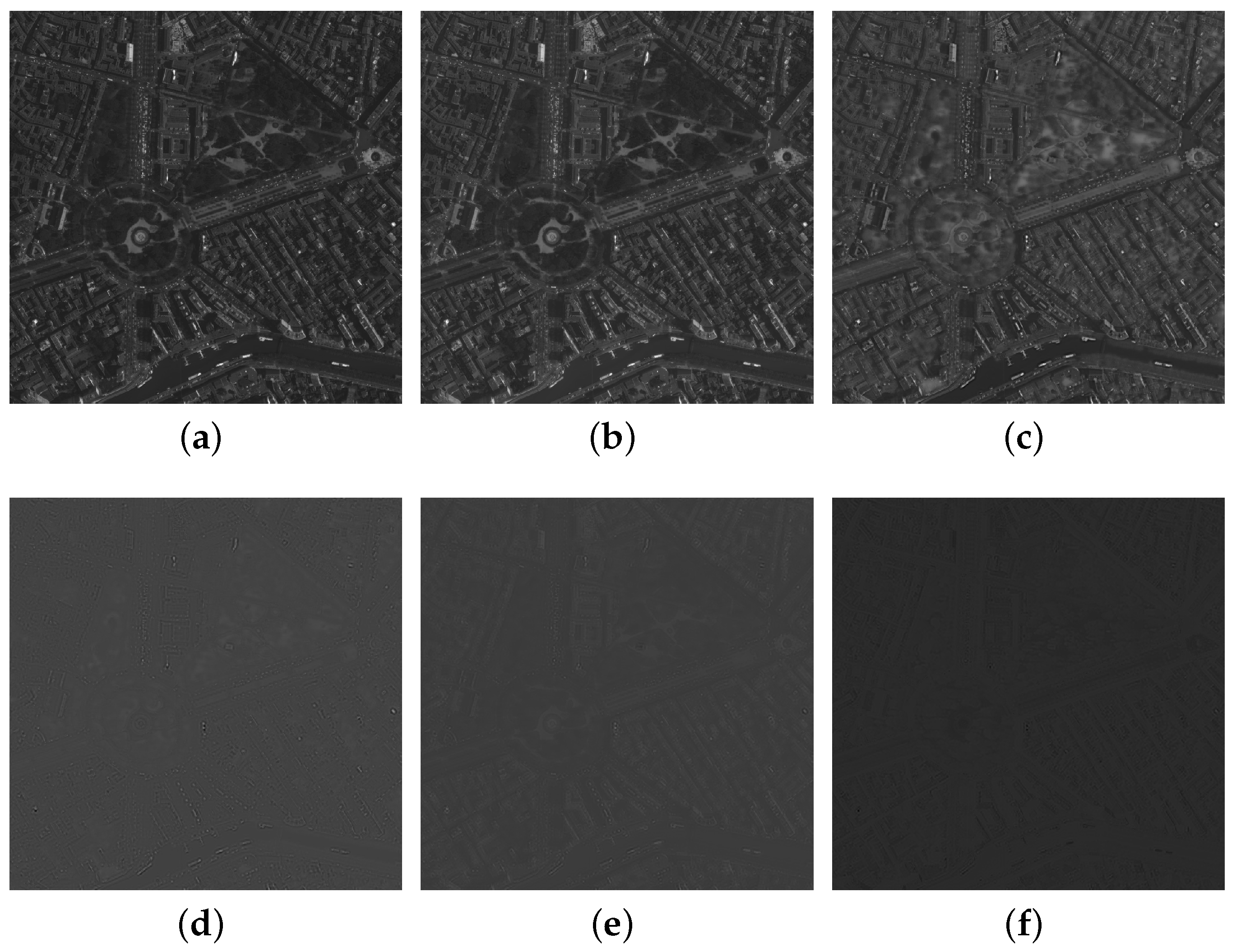
In Figure 6, we present I ( j ) , j = 1 , 2 , 3 , 4 , 5 , each being the result of the jth outer iteration of Algorithm 2 with respect to Pléiades dataset. To focus on spatial details, only the first channel of each image is shown. For each of the last four images, we subtract its intensities by the corresponding smallest value in the channel before normalization, since these images contain negative intensities which cannot be plotted by MATLAB directly. For better visualization, the normalization of these four images are implemented by dividing the largest intensity of I ( 2 ) since their absolute values are rather small compared with I ( 1 ) . From these visual results, we know that the outer iteration in Algorithm 2 is able to pick up more image details.
From Table 5, Table 6, Table 7 and Table 8, quantitative results of the proposed method with γ changing from 1 to 6 are listed. When γ = 1 , the proposed method essentially becomes Algorithm 1, which makes it convenient to compare it with the performance of Algorithm 2 directly. As expected, after combining Algorithm 1 with the iterative strategy, better quantitative performance is achieved, which can also be inferred from Figure 6.
We observe from Table 5, Table 6, Table 7 and Table 8 that the best quantitative performance is achieved at γ = 5 when γ is not too large, i.e., smaller than 6. An exception can be noticed in the case of SPOT-6 dataset, where the best performance is observed at γ = 4 . However, for the rest of the datasets, the case of γ = 5 outperforms other cases.
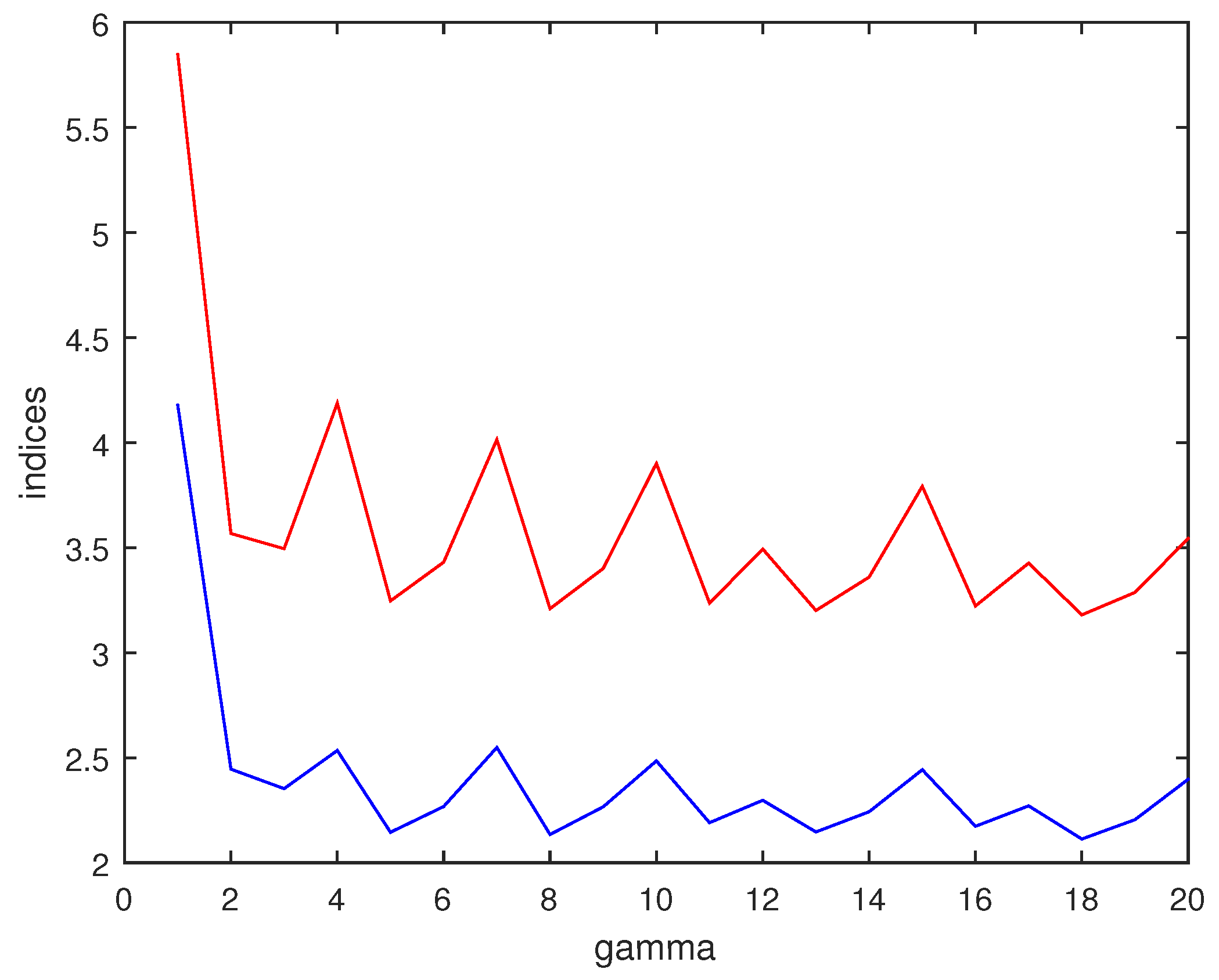
When we let γ goes even larger, things become different. This can be seen in Figure 7, which shows how indices vary when γ goes from 1 to 20. Since situation for all the tested datasets and all the indices is similar, we only present two indices related to Pléiades dataset here. From Figure 7, it is obvious that the curves of indices fluctuate when γ is larger than 3. However, it is also noticeable that there is not much improvement for the performance of Algorithm 2 corresponds to larger γ compared with the case of γ = 5 .
To explain this phenomenon, an iterative regularization algorithm [58] may be helpful, whose output signals become noisy if the outer iterations are not stopped properly, i.e., smaller than a threshold. And the authors explain that the phenomenon of noisiness is due to the influence of noisy input image. Despite the fact that the output images of Algorithm 2 do not necessarily degrade all the way when γ becomes larger than 5, the explanation of the similar phenomenon in [58] is enlightening. Therefore, we suggest that the output of Algorithm 2 is influenced significantly by the blurred upsampling multispectral image when γ is large enough, which leads to the fluctuation of numerical indices. Since the success of our iterative strategy has been preliminarily demonstrated by numerical results, an analysis of this conjecture can be explored in our future research. We simply set γ as 5 as a tradeoff of computational burden and the performance of the proposed algorithm, and also as a strategy to save the efforts of tuning.

4.4. Time Comparison with RKHS Method

Since we mentioned in Section 3 that the proposed model is supposed to simplify model (3), it is reasonable to expect a reduction in running time when comparing these two methods. Time cost of both methods for the four datasets can be examined in Table 9, whose values are presented in the unit of second. We point out that these results are obtained by running on the same laptap with 4GB RAM and 1.70GHz Intel(R) Core(TM) i5-4210U CPU as mentioned in the beginning of Section 4.
From the table, it can be validated that the proposed method is much less time consuming than RKHS method, which means the goal of reduction in computational burden and running time is achieved.

5. Conclusions

In this paper, a new iterative pan-sharpening approach is proposed for the fusion of panchromatic image and multispectral image. The proposed variational model inherits the framework of RKHS method but is essentially different. Instead of paying attention to modelling the unknown high resolution multispectral image in a complicated way, we utilize framelet technique in image restoration for more effectiveness of regularization. An iterative scheme similar to [22] is also employed to improve performance of the proposed algorithm. Experiments on data from Quickbird, Pléiades, WorldView-2, and SPOT are conducted for visual and numerical assessment. The results demonstrate that the proposed method outperforms several state-of-the-art pan-sharpening methods both visually and quantitatively. Meanwhile, it succeeds in reducing time cost compared with RKHS method.

Acknowledgments

The authors would like to thank the supports by NSFC (61772003, 61702083) and Fundamental Research Funds for the Central Universities (ZYGX2016KYQD142, ZYGX2016J132, ZYGX2016J129).

Author Contributions

Liang-Jian Deng and Zi-Yao Zhang conceived and designed the experiments. Zi-Yao Zhang, Liang-Jian Deng and Chao-Chao Zheng wrote the source code. Zi-Yao Zhang performed the experiments and wrote the paper. Ting-Zhu Huang, Liang-Jian Deng, Jie Huang and Xi-Le Zhao provided detailed advice during the writing process. Ting-Zhu Huang and Liang-Jian Deng supervised the whole process and improved the manuscript.

Conflicts of Interest

The authors declare no conflict of interest.

References

  1. Mohammadzadeh, A.; Tavakoli, A.; Valadan Zoej, M.J. Road extraction based on fuzzy logic and mathematical morphology from pansharpened IKONOS images. Photogramm. Rec. 2006, 21, 44–60. [Google Scholar] [CrossRef]
  2. Souza, C., Jr.; Firestone, L.; Silva, L.M.; Roberts, D. Mapping forest degradation in the Eastern Amazon from SPOT 4 through spectral mixture models. Remote Sens. Environ. 2003, 87, 494–506. [Google Scholar] [CrossRef]
  3. Carper, W.; Lillesand, T.; Kiefer, R. The use of intensity-hue-saturation transformations for merging SPOT panchromatic and multispectral image data. Photogramm. Eng. Remote Sens. 1990, 56, 459–467. [Google Scholar]
  4. Chavez, P.S., Jr.; Kwarteng, A.W. Extracting spectral contrast in Landsat thematic mapper image data using selective principal component analysis. Photogramm. Eng. Remote Sens. 1989, 55, 339–348. [Google Scholar]
  5. Laben, C.A.; Brower, B.V. Process for Enhancing the Spatial Resolution of Multispectral Imagery Using Pan-Sharpening. U.S. Patent 6011875, 2000. [Google Scholar]
  6. Xu, Q.; Li, B.; Zhang, Y.; Ding, L. High-fidelity component substitution pansharpening by the fitting of substitution data. IEEE Trans. Geosci. Remote Sens. 2014, 52, 7380–7392. [Google Scholar]
  7. Kang, X.; Li, S.; Benediktsson, J.A. Pansharpening with Matting model. IEEE Trans. Geosci. Remote Sens. 2014, 52, 5088–5099. [Google Scholar] [CrossRef]
  8. Shensa, M.J. The discrete wavelet transform: Wedding the à trous and Mallat algorithm. IEEE Trans. Signal Process. 1992, 40, 2464–2482. [Google Scholar] [CrossRef]
  9. Mallat, S. A theory for multiresolution signal decomposition: The wavelet representation. IEEE Trans. Pattern Anal. Mach. Intell. 1989, 11, 674–693. [Google Scholar] [CrossRef]
  10. Nason, G.P.; Silverman, B.W. The stationary wavelet transform and some statistical applications. In Wavelets and Statistics; Springer: New York, NY, USA, 1995; pp. 281–299. [Google Scholar]
  11. Burt, P.J.; Adelson, E.H. The Laplacian pyramid as a compact image code. IEEE Trans. Commun. 1983, COM-31, 532–540. [Google Scholar] [CrossRef]
  12. Starck, J.L.; Fadili, J.; Murtagh, F. The undecimated wavelet decomposition and its reconstruction. IEEE Trans. Image Process. 2007, 16, 297–309. [Google Scholar] [CrossRef] [PubMed]
  13. Nencini, F.; Garzelli, A.; Baronti, S.; Alparone, L. Remote sensing image fusion using the curvelet transform. Inf. Fusion 2007, 8, 143–156. [Google Scholar] [CrossRef]
  14. Price, J.C. Combining panchromatic and multispectral imagery from dual resolution satellite instruments. Remote Sens. Environ. 1987, 21, 119–128. [Google Scholar] [CrossRef]
  15. Palsson, F.; Sveinsson, J.R.; Ulfarsson, M.O. A new pansharpening algorithm based on total variation. IEEE Geosci. Remote Sens. Lett. 2014, 11, 318–322. [Google Scholar] [CrossRef]
  16. Zhao, X.L.; Wang, F.; Huang, T.Z.; Ng, M.K.; Plemmons, R. Deblurring and sparse unmixing for hyperspectral images. IEEE Trans. Geosci. Remote Sens. 2013, 51, 4045–4058. [Google Scholar] [CrossRef]
  17. Fang, F.M.; Li, F.; Shen, C.M.; Zhang, G.X. A variational approach for pan-sharpening. IEEE Trans. Image Process. 2013, 22, 2822–2834. [Google Scholar] [CrossRef] [PubMed]
  18. Fang, F.M.; Li, F.; Zhang, G.X.; Shen, C.M. A variational method for multisource remote-sensing image fusion. Int. J. Remote Sens. 2013, 34, 2470–2486. [Google Scholar] [CrossRef]
  19. He, X.; Condat, L.; Bioucas-Dias, J.; Chanussot, J.; Xia, J. A new pansharpening method based on spatial and spectral sparsity priors. IEEE Trans. Image Process. 2014, 23, 4160–4174. [Google Scholar] [CrossRef] [PubMed]
  20. Pan, Z.X.; Yu, J.; Huang, H.J.; Hu, S.X.; Zhang, A.W.; Ma, H.B.; Sun, W.D. Super-Resolution Based on Compressive Sensing and Structural Self-Similarity for Remote Sensing Images. IEEE Trans. Geosci. Remote Sens. 2013, 51, 4864–4876. [Google Scholar] [CrossRef]
  21. Masi, G.; Cozzolino, D.; Verdoliva, L.; Scarpa, G. Pansharpening by convolutional neural networks. Remote Sens. 2016, 8, 594. [Google Scholar] [CrossRef]
  22. Deng, L.J.; Vivone, G.; Guo, W.H.; Mura, M.D.; Chanussot, J. A variational pansharpening approach based on reproducible kernel Hilbert space and Heaviside function. In Proceedings of the IEEE International Conference on Image Processing (ICIP), Beijing, China, 17–20 September 2017. [Google Scholar]
  23. Aiazzi, B.; Baronti, S.; Selva, M. Improving Component Substitution Pansharpening Through Multivariate Regression of MS + Pan Data. IEEE Trans. Geosci. Remote Sens. 2007, 45, 3230–3239. [Google Scholar] [CrossRef]
  24. Deng, L.J.; Guo, W.H.; Huang, T.Z. Single image super-resolution via an iterative reproducing kernel Hilbert space method. IEEE Trans. Circuits Syst. Video Technol. 2016, 26, 2001–2014. [Google Scholar] [CrossRef] [PubMed]
  25. Zhu, X.X.; Bamler, R. A sparse image fusion algorithm with application to pan-sharpening. IEEE Trans. Geosci. Remote Sens. 2013, 51, 2827–2836. [Google Scholar] [CrossRef]
  26. Dong, B.; Zhang, Y. An efficient algorithm for l0 minimization in wavelet frame based image restoration. J. Sci. Comput. 2013, 54, 350–368. [Google Scholar] [CrossRef]
  27. Huang, J.; Donatelli, M.; Chen, R. Nonstationary iterated thresholding algorithms for image deblurring. Inverse Probl. Imaging 2013, 7, 717–736. [Google Scholar]
  28. Cai, J.F.; Dong, B.; Shen, Z.W. Image restoration: A wavelet frame based model for piecewise smooth functions and beyond. Appl. Comput. Harmon. Anal. 2016, 41, 94–138. [Google Scholar] [CrossRef]
  29. Shi, Y.; Yang, X.; Cheng, T. Pansharpening of multispectral images using the nonseparable framelet lifting transform with high vanishing moments. Inf. Fusion 2014, 20, 213–224. [Google Scholar] [CrossRef]
  30. Fang, F.M.; Zhang, G.X.; Li, F.; Shen, C.M. Framelet based pan-sharpening via a variational method. Neurocomputing 2014, 129, 362–377. [Google Scholar] [CrossRef]
  31. Ron, A.; Shen, Z. Affine systems in L2(ℝd): The analysis of the analysis operator. J. Funct. Anal. 1997, 148, 408–447. [Google Scholar] [CrossRef]
  32. Dong, B.; Shen, Z. MRA-Based Wavelet Frames and Applications; IAS Lecture Notes Series; The Mathematics of Image Processing: Park City, UT, USA, 2010. [Google Scholar]
  33. Cai, J.F.; Osher, S.; Shen, Z.W. Split Bregman methods and frame based image restoration. Multiscale Model. Simul. SIAM Interdiscip. J. 2009, 8, 337–369. [Google Scholar] [CrossRef]
  34. Elad, M.; Starck, J.; Querre, P.; Donoho, D. Simultaneous cartoon and texture image inpainting using morphological component analysis (MCA). Appl. Comput. Harmonic Anal. 2005, 19, 340–358. [Google Scholar] [CrossRef]
  35. Chambolle, A.; Pock, T. A first-order primal-dual algorithm for convex problems with applications to imaging. J. Math. Imaging Vis. 2011, 40, 120–145. [Google Scholar] [CrossRef]
  36. He, B.; Tao, M.; Yuan, X. Alternating direction method with Gaussian back substitution for separable convex programming. SIAM J. Optim. 2012, 22, 313–340. [Google Scholar] [CrossRef]
  37. Liu, J.; Huang, T.Z.; Selesnick, I.W.; Lv, X.G.; Chen, P.Y. Image restoration using total variation with overlapping group sparsity. Inf. Sci. 2015, 195, 232–246. [Google Scholar] [CrossRef]
  38. Deng, L.J.; Guo, W.H.; Huang, T.Z. Single image super-resolution by approximated Heaviside functions. Inf. Sci. 2016, 348, 107–123. [Google Scholar] [CrossRef]
  39. Ji, T.Y.; Huang, T.Z.; Zhao, X.L.; Ma, T.H.; Liu, G. Tensor completion using total variation and low-rank matrix factorization. Inf. Sci. 2016, 326, 243–257. [Google Scholar] [CrossRef]
  40. Chen, Y.; Huang, T.Z.; Zhao, X.L.; Deng, L.J.; Huang, J. Stripe noise removal of remote sensing images by total variation regularization and group sparsity constraint. Remote Sens. 2017, 9, 559. [Google Scholar] [CrossRef]
  41. Dou, H.X.; Huang, T.Z.; Deng, L.J.; Zhao, X.L.; Huang, J. Directional l0 sparse modeling for image stripe noise removal. Remote Sens. 2018, 10, 361. [Google Scholar] [CrossRef]
  42. Oden, J.T.; Glowinski, R.; Tallec, P.L. Augmented Lagrangian and Operator Splitting Method in Non-Linear Mechanics; Society for Industrial and Applied Mathematics: Philadelphia, PA, USA, 1989. [Google Scholar]
  43. Shi, W.; Ling, Q.; Yuan, K.; Wu, G.; Yin, W. On the linear convergence of the ADMM in decentralized consensus optimization. IEEE Trans. Signal Process. 2014, 62, 1750–1761. [Google Scholar] [CrossRef]
  44. Donoho, D. De-noising by soft-thresholding. IEEE Trans. Inf. Theory 1995, 41, 613–627. [Google Scholar] [CrossRef]
  45. Vivone, G.; Alparone, L.; Chanussot, J.; Dalla Mura, M.; Garzelli, A.; Licciardi, G.; Restaino, R.; Wald, L. A critical comparison among pansharpening algorithms. IEEE Geosci. Remote Sens. Lett. 2015, 53, 2565–2586. [Google Scholar] [CrossRef]
  46. Wald, L.; Ranchin, T.; Mangolini, M. Fusion of satellite images of different spatial resolutions: Assessing the quality of resulting images. Photogramm. Eng. Remote Sens. 1997, 63, 691–699. [Google Scholar]
  47. Chavez, P.S., Jr.; Sides, S.C.; Anderson, J.A. Comparison of three different methods to merge multiresolution and multispectral data: Landsat TM and SPOT panchromatic. Photogramm. Eng. Remote Sens. 1991, 57, 295–303. [Google Scholar]
  48. Vivone, G.; Restaino, R.; Dalla Mura, M.; Licciardi, G.; Chanussot, J. Contrast and error-based fusion schemes for multispectral image pansharpening. IEEE Geosci. Remote Sens. Lett. 2014, 11, 930–934. [Google Scholar] [CrossRef]
  49. Aiazzi, B.; Alparone, L.; Baronti, S.; Garzelli, A.; Selva, M. MTF-tailored multiscale fusion of highresolution MS and PAN imagery. Photogramm. Eng. Remote Sens. 2006, 72, 591–596. [Google Scholar] [CrossRef]
  50. Zeng, D.; Hu, Y.; Huang, Y.; Xu, Z.; Ding, X. Pan-sharpening with Structural Consistency and L1/2 Gradient Prior. Remote Sens. Lett. 2016, 7, 1170–1179. [Google Scholar] [CrossRef]
  51. Ghahremani, M.; Ghassemian, H. Nonlinear IHS: A promising method for pan-sharpening. IEEE Geosci. Remote Sens. Lett. 2016, 13, 1606–1610. [Google Scholar] [CrossRef]
  52. Alparone, L.; Wald, L.; Chanussot, J.; Thomas, C.; Gamba, P.; Bruce, L.M. Comparison of pansharpening algorithms: Outcome of the 2006 grs-s data-fusion contest. IEEE Trans. Geosci. Remote Sens. 2007, 45, 3012–3021. [Google Scholar] [CrossRef] [Green Version]
  53. Wang, Z.; Bovik, C. A universal image quality index. IEEE Signal Process. Lett. 2002, 9, 81–84. [Google Scholar] [CrossRef]
  54. Alparone, L.; Baronti, S.; Garzelli, A.; Nencini, F. A global quality measurement of pan-sharpened multispectral imagery. IEEE Geosci. Remote Sens. Lett. 2004, 1, 313–317. [Google Scholar] [CrossRef]
  55. Choi, M. A new intensity-hue-saturation fusion approach to image fusion with a tradeoff parameter. IEEE Trans. Geosci. Remote Sens. 2006, 44, 1672–1682. [Google Scholar] [CrossRef]
  56. Zhou, J.; Civco, D.L.; Silander, J.A. A wavelet transform method to merge Landsat TM and SPOT panchromatic data. Int. J. Remote Sens. 1998, 19, 743–757. [Google Scholar] [CrossRef]
  57. Aiazzi, B.; Alparone, L.; Baronti, S.; Garzelli, A. Context-driven fusion of high spatial and spectral resolution images based on oversampled multiresolution analysis. IEEE Trans. Geosci. Remote Sens. 2002, 40, 2300–2312. [Google Scholar] [CrossRef]
  58. Osher, S.; Burger, M.; Goldfarb, D.; Xu, J.; Yin, W. An iterative regularization method for total variation-based image restoration. Multiscale Model. Simul. 2005, 4, 460–489. [Google Scholar] [CrossRef]
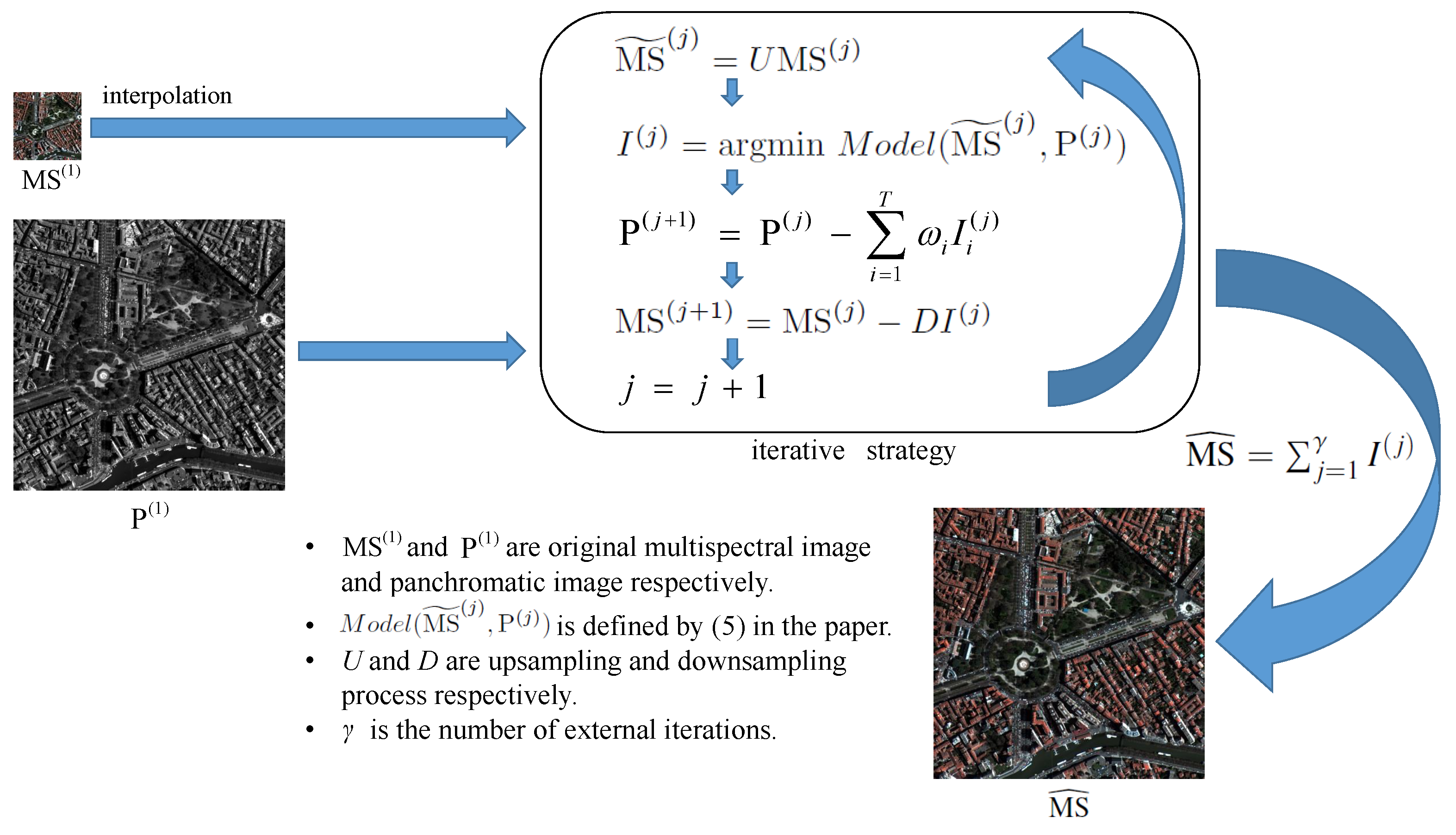
Figure 1. Framework of the proposed iterative pan-sharpening approach.
Remotesensing 10 00622 g001
Figure 2. Visual results for Quickbird dataset (4 bands, 512 × 512 ) obtained by different pan-sharpening methods. (a) Referential high resolution multispectral image, (b) PCA method, (c) GS method, (d) HPF method, (e) MTFGLP method, (f) PHLP method, (g) NIHS method, (h) RKHS method, (i) Proposed method.
Remotesensing 10 00622 g002
Figure 3. Visual results for Pléiades dataset (4 bands, 1024 × 1024 ) obtained by different pan-sharpening methods. (a) Referential high resolution multispectral image, (b) PCA method, (c) GS method, (d) HPF method, (e) MTFGLP method, (f) PHLP method, (g) NIHS method, (h) RKHS method, (i) Proposed method.
Remotesensing 10 00622 g003
Figure 4. Visual results for WorldView-2 dataset (4 bands, 800 × 800 ) obtained by different pan-sharpening methods. (a) Referential high resolution multispectral image, (b) PCA method, (c) GS method, (d) HPF method, (e) MTFGLP method, (f) PHLP method, (g) NIHS method, (h) RKHS method, (i) Proposed method.
Remotesensing 10 00622 g004
Figure 5. Visual results of the SPOT-6 dataset (4 bands, 1024 × 1024 ) obtained by different pan-sharpening methods. (a) Referential high resolution multispectral image, (b) PCA method, (c) GS method, (d) HPF method, (e) MTFGLP method, (f) PHLP method, (g) NIHS method, (h) RKHS method, (i) Proposed method.
Remotesensing 10 00622 g005
Figure 6. I ( j ) computed by Algorithm 2 for Pléiades dataset; (a) the first channel of the sum of I ( j ) , j = 1 , 2 , 3 , 4 , 5 ; (b) the first channel of I ( 1 ) ; (c) the first channel of I ( 2 ) ; (d) the first channel of I ( 3 ) ; (e) the first channel of I ( 4 ) ; (f) the first channel of I ( 5 ) .
Remotesensing 10 00622 g006
Figure 7. Performance of Algorithm 2 as γ increases, represented by SAM (red) and ERGAS (blue) with respect to Pléiades dataset.
Remotesensing 10 00622 g007
Table 1. Quantitative results for Quickbird dataset.
MethodSAMQ4QRASEERGASCCRMSEPSNR
PCA5.28120.77340.389521.58744.74530.75200.124618.0910
GS2.31620.85100.834512.38412.93100.94330.071522.9177
HPF2.17270.85610.82998.54652.06810.94200.049326.1392
MTFGLP2.27670.87560.83996.12731.62870.94390.035429.0296
PHLP5.00530.81840.773611.55262.90200.90770.066723.5214
NIHS2.90600.72120.752114.49553.42470.91610.083721.5503
RKHS3.06820.87250.83807.49551.98680.94130.043327.2789
Proposed2.24220.88160.85255.12651.46050.94840.029630.5785
Table 2. Quantitative results for Pléiades dataset.
MethodSAMQ4QRASEERGASCCRMSEPSNR
PCA9.54570.78290.838732.80338.05070.92760.063723.9147
GS9.12220.83360.890028.80606.49170.96450.056025.0434
HPF10.86940.83760.924327.84496.75830.97220.054125.3382
MTFGLP4.79250.90630.965314.65153.24700.98010.028530.9155
PHLP3.95580.77490.918623.63494.83080.95080.045926.7620
NIHS5.80530.78070.895432.94086.60980.95000.064023.8784
RKHS3.82940.90710.971012.05422.50880.98290.023432.6103
Proposed3.24650.92780.977510.38862.14520.98570.020233.9019
Table 3. Quantitative results for WorldView-2 dataset.
MethodSAMQ4QRASEERGASCCRMSEPSNR
PCA7.11370.92560.913717.45243.99600.96080.077822.1796
GS5.22540.93120.943813.19913.20490.97760.058824.6058
HPF4.13520.91850.94879.95632.49250.98320.044427.0547
MTFGLP4.39260.93720.95319.13862.38520.98570.040727.7991
PHLP4.07160.78790.905813.55403.29780.97200.060424.3753
NIHS1.71280.77510.878129.66505.67490.96450.132317.5718
RKHS5.35240.93400.954611.77162.95880.98640.052525.6000
Proposed3.51760.94410.96476.68181.78290.98790.029830.5188
Table 4. Quantitative results for SPOT-6 dataset.
MethodSAMQ4QRASEERGASCCRMSEPSNR
PCA8.41790.85940.900223.38636.16770.96530.056524.9547
GS7.05580.89760.924825.66535.27510.98040.062024.1470
HPF7.75390.87070.917226.00125.52110.97270.062824.0340
MTFGLP3.81180.91620.936220.51744.16870.97950.049626.0915
PHLP5.88270.77680.904421.15174.89400.96590.051125.8270
NIHS3.80080.78480.877034.39836.43430.95880.083121.6032
RKHS2.59380.92660.953011.81522.81060.98420.028630.8851
Proposed3.28180.93000.956610.86402.63350.98430.026331.6141
Table 5. Quantitative results for Quickbird dataset with different numbers of outer iterations.
CaseSAMQ4QRASEERGASCCRMSEPSNR
γ = 1 3.60360.86330.827410.08522.51460.93930.058224.7013
γ = 2 2.61970.87960.84686.37181.68390.94710.036828.6898
γ = 3 2.28130.88160.84995.48271.51650.94760.031629.9951
γ = 4 2.35630.88280.84965.29381.53540.94650.030630.2996
γ = 5 2.24220.88160.85255.12651.46050.94840.029630.5785
γ = 6 2.33820.88220.85005.18631.51450.94650.029930.4778
Table 6. Quantitative results for Pléiades dataset with different numbers of outer iterations.
CaseSAMQ4QRASEERGASCCRMSEPSNR
γ = 1 5.84700.87580.938319.24514.17790.97540.037428.5467
γ = 2 3.56710.91870.972511.81892.44540.98300.023032.7816
γ = 3 3.49470.92440.974611.57542.35270.98390.022532.9624
γ = 4 4.18770.92470.973112.55062.53430.98430.024432.2598
γ = 5 3.24650.92780.977510.38862.14520.98570.020233.9019
γ = 6 3.43060.92750.976110.96752.26760.98540.021333.4309
Table 7. Quantitative results for WorldView-2 dataset with different numbers of outer iterations.
CaseSAMQ4QRASEERGASCCRMSEPSNR
γ = 1 5.27610.93380.948412.18163.03190.98160.054325.3026
γ = 2 4.27520.94220.96088.28562.19550.98720.036928.6502
γ = 3 3.78840.94360.96377.14681.88660.98770.031929.9344
γ = 4 3.66760.94390.96407.34701.96810.98780.032829.6944
γ = 5 3.51760.94410.96476.68181.78290.98790.029830.5188
γ = 6 3.26130.94330.96526.74561.84070.98760.030130.4363
Table 8. Quantitative results for SPOT-6 dataset with different numbers of outer iterations.
CaseSAMQ4QRASEERGASCCRMSEPSNR
γ = 1 6.86770.91090.928423.48894.83190.98030.056824.9167
γ = 2 3.66020.92700.950413.60973.10980.98240.032929.6569
γ = 3 2.83940.92870.953510.99222.62970.98240.026631.5123
γ = 4 2.62450.92680.951810.11822.50810.98190.024532.2318
γ = 5 3.28180.93000.956610.86402.63350.98430.026331.6141
γ = 6 3.85260.92950.955810.87892.68520.98410.026331.6022
Table 9. Running time(s) of RKHS and the proposed method on four datasets.
MethodQuickbirdPléiadesWorldView-2SPOT-6
RKHS7263.2227882.8716559.9331576.65
Proposed207.71851.11512.47863.59