Article

Using Image Texture and Spectral Reflectance Analysis to Detect Yellowness and Esca in Grapevines at Leaf-Level

1
INRA, UMR 1347 Agroecology, 21000 Dijon, France
2
Roullier Group, 35400 Saint-Malo, France
*
Authors to whom correspondence should be addressed.
Remote Sens. 2018, 10(4), 618; https://doi.org/10.3390/rs10040618
Submission received: 6 March 2018 / Revised: 10 April 2018 / Accepted: 17 April 2018 / Published: 18 April 2018
(This article belongs to the Section Remote Sensing Image Processing)

Abstract

:
Plant diseases are one of the main reasons behind major economic and production losses in the agricultural field. Current research activities enable large fields monitoring and plant disease detection using innovative and robust technologies. French grapevines have a reputation for producing premium quality wines, however, these major fruit crops are susceptible to many diseases, including Esca, Downy mildew, Powdery mildew, Yellowing, and many others. In this study, we focused on two main infections (Esca and Yellowing), and data were gathered from fields that were located in Aquitaine and Burgundy regions, France. Since plant diseases can be diagnosed from the properties of the leaf, we acquired both Red-Green-Blue (RGB) digital image and hyperspectral reflectance data from infected and healthy leaves. Biophysical parameters that were produced by the PROSPECT model inversion together with texture parameters compiled from the literature were deduced. Then we investigated their relationship to damage caused by Yellowing and Esca. This study examined whether spectral and textural data can identify the two diseases through the use of Neural Networks. We obtained an overall accuracy of 99% for both of the diseases when textural and spectral data are combined. These results suggest that, first, biophysical parameters present a valid dimension reduction tool that could replace the use of complete hyperspectral data. Second, remote sensing using spectral reflectance and digital images can make an overall nondestructive, rapid, cost-effective, and reproducible technique to determine diseases in grapevines with a good level of accuracy.

Graphical Abstract

1. Introduction

Traditionally, laboratory-based diagnostic methods and symptomology are the main crop disease detection techniques. Biological methods include Polymerase Chain Reaction (PCR), Enzyme Linked Immuno Sorbent Assay (ELISA), fluorescence in situ hybridization, and biomarker-based detection technology. These techniques are however destructive and time-consuming. Visual inspection, on the other hand, is a subjective procedure, since it depends on the pathologist’s experience and it is affected by temporal change. Moreover, visual diagnosis is expensive, mainly in the case of wide canopies. Symptoms are generally a good indicator of a disease, however, it is not advised to make a decision that is only based on visual assessment. Hence, traditional crop disease diagnosis approaches lack precision, and developing alternatives seem to be essential.
In recent years, numerous non-destructive sensing technologies have been implemented to assess the physiological status of vegetation and to respond to the need for the automatic identification of diseases. When an infection occurs, the foliar concentration of pigments and biochemical components is altered [1,2]. As a result, the infected leaf reflectance in the Visible (VIS) and (Near-Infrared) NIR regions of the electromagnetic spectrum is no longer perfect and similar to a healthy reflectance. Many studies confirmed that reflectance data can be considered as a tool for damage quantification in crops. The work done in [3] concluded that the spectral reflectance of leaves corresponding to three kinds of fungal diseases were significantly different. A study on Yellow mosaic disease in soybean fields showed the difference in spectral reflectance between healthy and diseased cases. It enabled the identification of a single sensitive band and a spectral ratio for satellite in-field monitoring of the disease [4]. Seven spectral bands at the leaf-level and one band at canopy-level were identified by [5] for assessing the infestation level of rice leaf folder damage through the analysis of hyperspectral data gathered from healthy and infected sample leaves.
Biophysical parameters can be generated from high dimensional raw reflectance data using the PROSPECT model inversion, reducing the dimensionality of the spectral measurements. Researchers have adopted Radiative Transfer Models (RTM) for many applications. For example, the study in [6] demonstrated that RTM, together with hyperspectral (HS) airborne imaging, can be of great importance to determine the Leaf Area Index in grassland.
In addition to spectral information, digital image analysis is an effective and noninvasive method. It can produce information from computerized images for disease detection purposes. Texture refers to visual patterns or spatial arrangements of pixels that intensity or color of pixel alone cannot sufficiently describe. It corresponds to both brightness values and pixel locations. The texture feature information can reflect the intensity change of pixels, distinguishing and recognizing objects. AL-Hiary et al. proposed in [7] a robust technique for the recognition of five plant leaf diseases (Early scorch, Cottony mold, Ashen mold, late scorch, and tiny whiteness) using texture extraction from digital images. Furthermore, regions that were contaminated by three diseases (due to green stink bug, bacteria angular, Ascochyta blight virus) that were found in cotton leaves images in [8] were detected by defining a set of features and feeding them to a classifier. For more details about the different approaches for diagnosis of plant leaf diseases through digital image processing, refer to the review that is reported in [9].
Other studies focused on combining spectral and textural data for the sake of classifying crop infections. For example, Xie et al. [10] extracted texture parameters from hyperspectral images and investigated both spectrum and texture for early blight disease detection on an eggplant. Another study of Xie et al. [11] established detection models that were based on texture features. These were extracted from five multispectral images and gave good classification accuracies.
In our paper, we focused on grapevine disease detection, which is a complicated task because different vine infections can sometimes introduce comparable symptoms [12]. We considered two grapevine diseases in our study: Esca and yellowing of the grapevine and data were acquired from two different regions in France. Esca of the grapevine is a type of grapevine trunk diseases. In the last years, several European wine countries such as France, Italy and Spain have noted an increase of occurrence of the disease. Li et al. [13] assessed the nature of Esca spread within commercial vineyards in Bordeaux region, France for a long period of time. Another work was carried out in [14] from 2004 till 2006 in five mature vineyards in Aquitaine Province, France to monitor Esca occurrence. Leaf symptoms mainly appear as a stripe pattern (Figure 1), they can begin to emerge any time during the growing season, but they are mostly seen during July and August. When looking inside the trunks and main branches, a cross-sectional cut of symptomatic shoots uncovers the concentric rings of dark spots [15,16].
There are two forms of the Esca disease, which can be distinguished depending on their severity and their rapidity of appearance. The first is a chronic form and the second is an acute form (also called apoplexy): a severe type of Esca; once contaminated, the grapevines rarely recover. For more details on the syndrome development, refer to Mugnai et al. [17]. Traditional cultural methods to prevent Esca are based on chemical control using various fungicides.
The Yellowing of the grapevine, on the other hand, is transmitted by planthoppers and leafhoppers through an injection of contaminated saliva. There is no remedy for grapevine yellows that will definitively treat the plant. Preventing the spread of the disease is a currently used approach. Indeed, infected vines are removed, restraining them from becoming a source of infection for feeding insects [18]. An alternative solution might be to eliminate the insects that transmit the disease by massively applying pesticides. Yellowing of the grapevine alters the development of plants. It produces identical symptoms and affects many plant parts, such as fruit, growing points, leaves, and canes. Usually a combination of symptoms will develop on contaminated plants. Discoloration of leaves (red for red-berried varieties and yellow for yellow-berried varieties) might be the most noticeable symptom. Infected leaves also roll-up and become twisted (Figure 2). Canes do not ripen very well and present green-brown sections; flowers dry out and fruits might drop easily on some varieties.
“Flavescence Dorée” (FD) is the contagious type of yellowing of the grapevine, detailed information about FD can be found in [19].
The aim of this paper was to study the feasibility of detecting Esca and yellowing of the grapevine using spectral and texture data. On one side, we presented different methods and functions for performing a PROSPECT model inversion to calculate the biophysical parameters. On the other side, we compared the efficiencies of texture and spectral analyses in classifying sample leaves. The novelty of this work relies on suggesting the optimal association of methods and functions that are used for the PROSPECT model inversion. Furthermore, to our knowledge, this is the first study that attempts to test the ability of combining spectral (biophysical parameters) and image data (texture parameters) in distinguishing damaged grapevine leaves from healthy ones. The results of using biophysical parameters are also compared to using complete hyperspectral measurements.
The article is organized as follows: Section 1 describes how the measurements were acquired, Section 2 introduces the spectral analysis along with the textural analysis. Section 3 states and discusses the results, and finally, Section 4 presents the conclusion along with future works.

2. Materials and Methods

2.1. Data Acquisition

Figure 3, shows different grapevine growing regions in France, however, we only conducted tests in Burgundy and Aquitaine regions. In the Burgundy region, we examined a white berried variety of Chardonnay grapevines that were infested with Yellowing. In the Nouvelle Aquitaine region, we investigated a red-berried variety of Cabernet Sauvignon grapevines infested with Esca. Two field surveys were performed in Bordeaux (Clement castle, Latitude: 44.806031, Longitude: −0.647603, Elevation: 37 m) in the mornings of the 12th of July and the 19th of September 2017 and in Burgundy (Macôn-Plottes sector, Latitude: 46.530431, Longitude: 4.871726, Elevation: 269 m) in the mornings of the 17th of August and the 25th of September 2017. Traditional cultural practices are applied in the two tested fields.
From each variety, we selected four diseased and four healthy grapevines and one to four leaves per grapevine were taken like samples. We took four spectral measurements on each sample leaf and averaged them; the corresponding locations are shown in Figure 4. This procedure is adopted to take into account leaves’ spectral variability. Moreover, we captured one digital RGB image per leaf. We selected infested leaves to get a complete and representative range of diseases symptoms at the end of the experiments. For the healthy group, we selected healthy leaves of different ages.
All of the labeled leaves were visually inspected by a plant pathologist from the Interprofessional Office of Burgundy Wines (BIVB) and Pape Clement, and they were classified according to disease symptoms presence and intensity. In total, there were 25 diseased and 30 healthy Cabernet Sauvignon leaves; and, 35 diseased and 35 healthy Chardonnay leaves. In order to ensure timely follow-up, the grapevines were located using a GPS and leaves were also labeled.

2.2. Reflectance Measurements and Digital Images

A portable Spectroradiometer (FieldSpec 3, Analytical Spectral Devices, Boulder, CO, USA) was used to obtain spectral reflectance measurements of adaxial leaf surfaces. Measurements were made on each leaf alone using a contact plant probe attachment, which is essentially a closed chamber with an internal light source that is specially made for sensible vegetative surfaces. The spectral resolution of the instrument varies from approximately 3 nm at 700 nm to 10 nm at 1400 nm wavelengths or longer; however, the spectra are interpolated by the spectrometer software to 1 nm intervals. Therefore, each measurement generated a spectrum with values that were between 350 nm and 2500 nm at 1 nm increments. The instrument was warmed up for at least 20 min prior to acqusitions. Calibration was performed to absolute reflectance using a Teflon calibration disk. The number of samples for Spectrum was set to 30, the number of samples for Dark Current and White Reference were set to 100. The measurements were made within approximatively four hours of field work.
A digital camera Sony Alpha 5000 with 20 Mpixels resolution was used to acquire the RGB images of each leaf. A uniform color board was placed behind the leaf prior to image acquisition to facilitate the analysis (Figure 5).

2.3. Spectral and Image Data Analysis for Disease Detection

The complete approach that is applied in this paper is summarized in Figure 6.
The first step of our workflow is the computation of biophysical parameters using PROSPECT model inversion requiring the hyperspectral spectrum. In same time, texture parameters is estimated from RBG image data. Both information are merged, and are used in a classification neural networks predicting health status of the leaf. The choice of the method and the function for the PROSPECT model inversion will be detailed next.

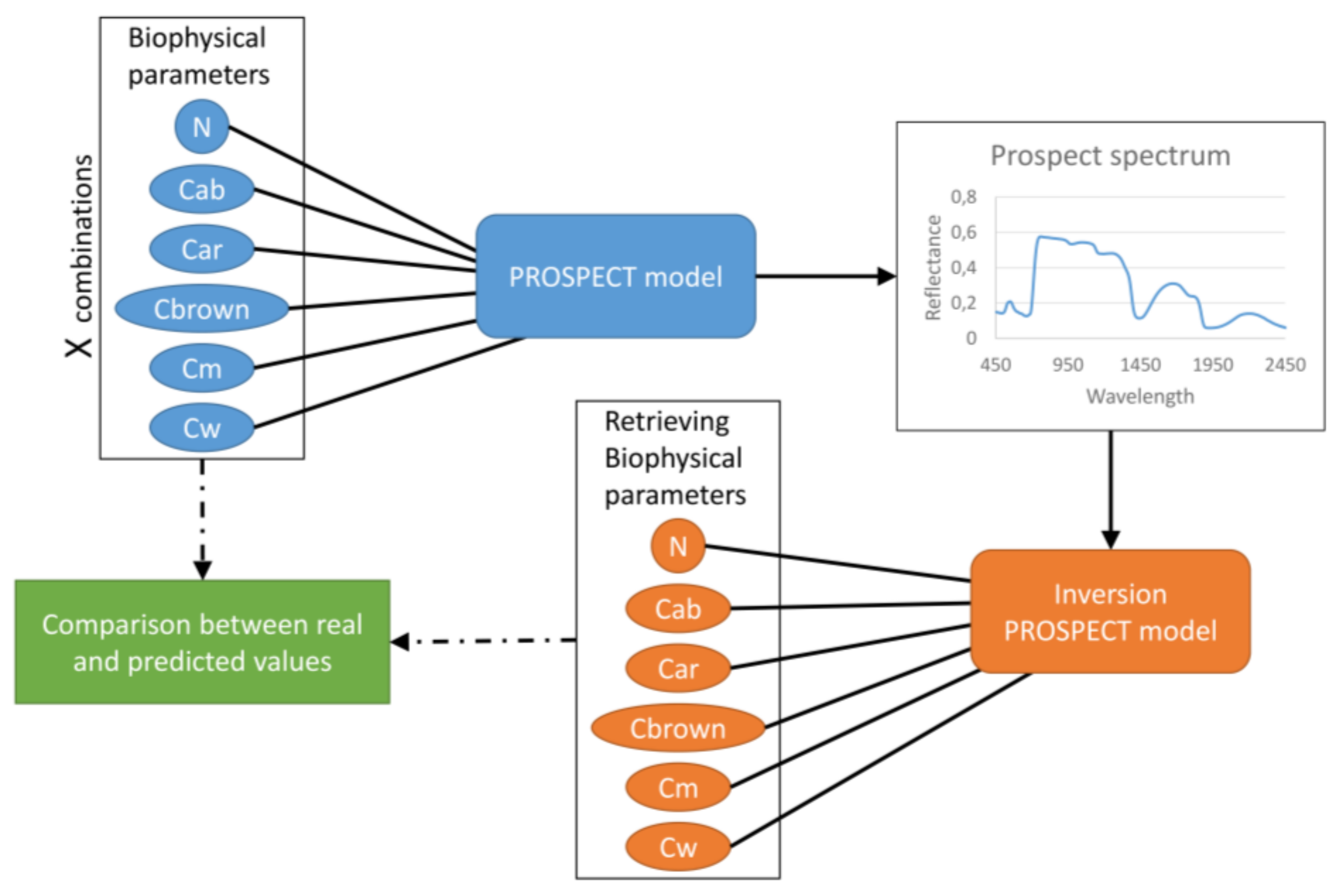
2.3.1. PROSPECT Model

PROSPECT is an empirical model of leaf optical properties that is based on relationships between spectral information and laboratory measurements, details about its development could be found in [20]. When working on the canopy scale, it is usually coupled with the SAIL radiative transfer model under a natural environment to take into account the inclinations of leaves, the solar position, and the sensor position. Using some variables, PROSPECT recreates two spectral information, a directional–hemispherical reflectance and a directional–hemispherical transmittance in the 400–2500 nm range. The early versions of the model need only three variables (N parameter, chlorophyll content, and water content). The lastest PROSPECT model that is employed in this work requires six variables to be launched. Each one of those variables are biophysical parameters representing the characteristics of a plant (N, Cab, Car, Cbrown, Cw, Cm). N represents the interactions between electromagnetic radiation and a plant’s leaves. It is dependent on whether a plant belongs to dicotyledonous or monocotyledonous families. Grapevines, in particular, are dicotyledonous plants. Cab, Car and Cbrown are chlorophyll, carotenoids and brown pigments, respectively. They represent foliar pigmentations. Cw and Cm correspond to the equivalent water thickness and the amount of dry matter, respectively. For more details, refer to [21], in which Feret et al. explained precisely the different parameters. In this work, we used the PROSPECT_5b model and we only focused on spectral reflectance, since the transmittance data were not collected during our acquisition campaigns.

2.3.2. Biophysical Parameters (BPs) Calculation

PROSPECT is a physical model that is simulating directional-hemispherical reflectance and transmittance. Although other RTM exist, PROSPECT is one of the most widely used [22]. The aim of the PROSPECT model inversion is to predict plant biophysical parameters from spectral data. Previous studies applied Look Up Tables (LUT) [23,24,25]. For example, a LUT-I with mean of best 10% solution was employed in [26] for RTM inversion. Other studies applied the artificial neuronal network (ANN) [27]. Since the above-mentioned techniques require performing many iterations to find a similar reflectance, they need time-consuming processing and a computer with a high extensive processing power.
It is possible to predict the biophysical variables within a short time by using an optimization approach. The basic concept of an optimization approach is to minimize a function of “n” variables by some iterations for solving the function and converging it towards a unique solution. There are two categories of methods that can be applied, unconstrained and constrained minimizations. Studies [21,28,29] have used a multi-start downhill simplex method that was developed by [30] and a constrained Powell’s method. Although the methods that they used were unconstrained ones, they constrained them somehow by using a specific algorithm. Indeed, without any constraints being applied, the inversion will be an “ill-posed” problem and getting trapped at a local minimum can mask a global minimum. Two important points need to be considered when the model inversion is applied. First, as indicated in [29], it is possible to obtain various combinations of input parameters for similar reflectance spectra, hence, it is necessary to know a range of different biophysical parameters. Second, caution should be taken when considering the initial values of parameters, because bad initial values lead to impractical results.
RMSE (Equation (1)) is commonly used as a minimization function. Most of the studies used different inversion methods, but they have employed the RMSE function, claiming that it is the best. However, we decided to investigate several other minimization functions: RMSE function (Equation (1)), Spectral Angle Mapper (SAM) function (Equation (2)), and Spectral Correlation Mapper (SCM) function (Equations (3) and (4)) [31], as follows:
RMSE = λ ( R m e s u r e d ( λ ) R m o d e l ( λ ) ) ² n
SAM = cos 1 ( λ ( R m e s u r e d ( λ )   R m o d e l ( λ ) ) R m e s u r e d ( λ )   R m o d e l ( λ ) )
R ( M e s u r e d ,   M o d e l ) = λ ( R m e s u r e d ( λ ) R m e s u r e d ( λ ) ¯ ) ( R m o d e l ( λ ) R m o d e l ( λ ) ¯ )   λ ( R m e s u r e d ( λ ) R m e s u r e d ( λ ) ¯ )   λ ( R m o d e l ( λ ) R m o d e l ( λ ) ¯ )
SCM = 1 1 + R ( M e s u r e d ,   M o d e l ) 2
where Rmesured(λ) and Rmodel(λ) are the reflectance directly given by the model and the reflectance after the model inversion, respectively.
Furthermore, we tested different types of methods in our study. Three constrained methods were considered: the first one was based on Broyden-Fletcher-Goldfarb-Shanno (L-BFGS-B), the second is the Sequential Least Squares Programming (SLSQP), and the third is the Truncated Newton (TNC). An unconstrained method (Nelder-Mead) was also applied and the performances of all the methods was compared. L-BFGS-B derivates from BFGS, it is a method that solves nonlinear optimization problems without constraints. Zhu et al. ameliorated it in [32] to comply with the addition of constraints. SLSQP method is a sequential least squares programming algorithm that uses the Han–Powell quasi–Newton method with a BFGS update [33]. An optimizer uses a slightly modified version of Lawson and Hanson’s nonlinear least-squares solver (NNLS). The last constrained method applied is the TNC method that is known as Hessian-free optimization [34], it is based on the Newton equations that are solved with an iterative algorithm. Nelder-Mead is an unconstrained method using basically a global minimization technique [30], which begins without predetermined values and at each iteration it compares function values at n + 1 level. We will not present more details about the different methods mentioned, since it is not the goal of our work.
The PROSPECT-5b model was applied by obtaining combinations of values of BPs from Table 1, depending on the range of each parameter. Nevertheless, not all of the combinations exist in reality, and for some of them, PROSPECT-5b cannot predict reflectance values from 400 nm to 2500 nm. These extreme cases are eliminated before inversion prediction. In this work, the transmittance, which is usually provided by the model, was not taken into account because it was not measured during our acquisition campaigns.
A total of 221,184 theoretical combinations of BPs was first created, depending on a range for each BP and then the PROSPECT-5b model calculated the spectra that are associated to each one of these combinations. A total of 192,215 combinations was retained because PROSPECT-5b model could not create full spectral signature for all of the combinations. Then, spectral information obtained were applied to predict again the biophysical parameters with different variants of PROSPECT model inversion (various associations of methods and functions). The BPs that were produced by different inversion models were compared with the initial BPs from the Table 1, using a linear regression. The corresponding workflow is presented in the Figure 7.
Python programming language was used to implement the different algorithms, along with libraries like PROSAIL and Scipy.

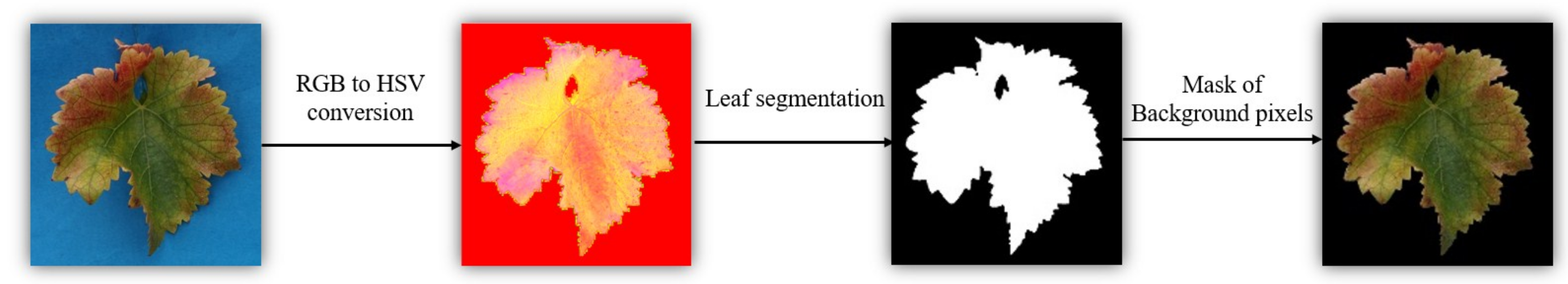
2.3.3. Pre-Processing of Digital Images

Figure 8 presents the different steps of the pre-processing strategy.
• RGB to HSV conversion
First, RGB images were converted to Hue Saturation Value (HSV) space through a non-linear transformation. This color space was selected since it is a good descriptor that is close to human perception. Hue describes an actual color as perceived, saturation is the purity of a color, and value means the lightness or darkness of a color.
v = max ( r , g , b )
s = { ( v min ( r , g , b ) × 255 ) / v v 0 0 v = 0 }
h = { ( g b ) × 60 s v = r 180 + ( b r )   ×   60 s v = g 240 + ( r g ) × 60 s v = b }
i f   h < 0 t h e n   h = h + 3 = 60
where r, g, and b represent pixel values of red, green, blue (RGB) color of image, respectively, and h, s, and v represent the new color channels in the HSV color space.
• Leaf segmentation
After color space conversion, a background subtraction was performed. The goal is to divide the image into two classes (background and leaf). The leaf was segmented from each HSV converted image using K-means algorithm. K-means is an iterative clustering algorithm that is well-used in many applications. It aims to partition a given set of patterns into different groups. The patterns belonging to the same cluster are similar and are distinguishable from those that are belonging to another cluster. The condition of clustering is to minimize the sum of squared distance from the points inside the cluster to its centroid.
• Mask of background pixels
K-means segments the images into two distinct regions, then the background pixels are set to zero, and only the pixels relative to the leaf are kept and used in the next steps of the analysis.

2.3.4. Co-Occurrence Matrices

Grey Level Co-occurrence Matrix (GLCM) is one of the most frequently used approaches for texture analysis. It can describe the essential characteristics of an image related to second order statistics that were introduced by Haralick [35].
Many scientific studies applied texture parameters from GLCMs for disease classification of various crop applications. The research [36] investigated the use of texture features that were extracted from hue, saturation, and intensity color space for the classification of citrus leaves under laboratory conditions. The research [37] studied diseases from eight species (banana, beans, jackfruit, lemon, mango, potato, tomato, and sapota) and showed that the algorithm could classify diseases with an accuracy of 94%. Focusing more on the grapevine crops, Sannaki et al. [38] studied downy mildew and powdery mildew in their experiments. Disease diagnosis was possible by applying image processing and artificial intelligence techniques.
GLCMs can be computed by defining a neighbor relationship between pixels. A distance step length d and a direction θ should be determined to create the co-occurrence matrix G(i, j|d, θ). An element (i,j) of a matrix G is a frequency of appearance of grey-tone j near the reference grey-tone i within an image at a defined distance and direction. The GLCM is a square matrix where the number of rows and columns equals the number of gray levels that are considered.
In this study, symmetrical GLCMs were constructed for each single channel image (H, S, and V) and were calculated for (θ = 0°, θ = 45°, θ = 90°, and θ = 135°) with an offset of 1 pixel.

2.3.5. Texture Parameters (TPs) Calculation

A set of features that were derived from four directional symmetrical GLCMs are considered for texture characterization. Based on a co-occurrence matrix, we can extract texture features, called second order statistical features. Athough Haralick proposed 14 different features, it is advised to select some of them for analysis to avoid redundancy among them. We selected contrast, correlation, energy, and homogeneity in this study [39,40].
Contrast (K) measures the local variations in gray level from a pixel to its neighbor in an image. It shows a texture fineness.
K = i , j ( i j ) 2 p ( i , j )
Correlation (R): measures the linear dependence of gray-levels in a co-occurrence matrix or in other words, a correlation intensity between neighboring pixels.
R = i , j ( i μ i ) ( j μ j ) p ( i , j ) σ i σ j
µi and µj are the averages of row i and column j in a GLCM, respectively. σi and σj are the standard deviations of row i and column j in the GLCM, respectively.
Energy (E) known as an angular second moment, it is simply the sum of squared elements in the GLCM. It measures the uniformity of an image.
E = i , j p ( i , j ) 2
Homogeneity (H) is a measure of closeness of a distribution of elements in the GLCM to the diagonal. Homogeneity is unity for a diagonal GLCM. This is the case where all of the pixels in the original image have the same value as their neighbor.
H = i , j p ( i , j ) 1 + | i j |

2.3.6. Classification: Neural Networks

Choosing the most appropriate classifier for an application is a tricky task because there are hundreds of classifiers in the scientific literature. We used in this research Neural Networks (NN) as a classification tool, more details about their theory can be found in [41]. NN is a well-known technique that has shown successful results in many real applications, specifically in the agricultural field. For example, authors in [42] collected data from Florida grapefruit, orange, and tangerine varieties using a color vision system and used various neural network classification methods to detect blemish-related features for the citrus fruit.
In particular, Back Propagation Neural Networks (BPNN) is a mathematical model consisting of a number of highly interconnected neurons that are organized into three parts: input layer, hidden layer, and output layer. At the training phase, the observations are provided to the network and the network is trained to produce a desired set of outputs. The network adjusts its variable parameters, the connection weights, and biases in order to produce the aimed mapping between the input and outputs patterns through the sum of error squares.
We have mixed data from the first and the second field survey in order to obtain a larger number of measurements. We tested the BPNN classification when considering hyperspectral data (complete spectra). In this case, we had 2151 features corresponding to the reflectance at each wavelength (350–2500 nm). Then, we applied the BPNN classification for biophysical parameters, consisting of six features: N, Cab, Car, Cbrown, Cw, and Cm. Furthermore, the BPNN was applied to texture parameters; here, 12 features are tested corresponding to: Contrast, Correlation, Energy, and Homogeneity extracted from the three bands of each HSV image. Finally, we combined biophysical with texture data after normalization to obtain in total 18 features and applied the same classification procedure to them. A BPNN consisting of one hidden layer with 10 neurons was used and the classification was repeated 20 times to insure the stability of the results.
Since the overall accuracy of a classification does not take into account the proportion of agreement between data sets that is due to chance alone and a difference in the numbers of positive and negative data, F-Measure (FM), and area under the Receiver Operating Curve (ROC) are an additional evaluation of the classification. Precision is the number of true positives divided by the total number of elements that are considered as belonging to the positive class. On the other hand, recall (R) is the number of true positives divided by the total number of elements that actually belong to the positive class. The harmonic mean of precision and recall, called the traditional F-measure or balanced F-score, combines precision and recall, as follows:
P = TP TP + FP
R = TP TP + FN
FM = 2 × P × R P + R
where true positive (TP) are the observations that are correctly classified as belonging to the positive class. False Positives (FP) are observations wrongly classified as belonging to the positive class. False Negatives (FN) are observations that are not classified as belonging to the positive class while they should have been.
When plotting on a single graph, the False Positive Rate (FPR) values on the abscissa and the True Positive Rate (TPR) values on the ordinate, the resulting curve is called ROC (Receiver Operating Characteristic) curve. The Area under ROC (AUC) refers to the area under that curve.
TPR = TP TP + FN
FPR = FP FP + TN
where True Negative (TN) are the observations that are correctly classified as belonging to the negative class.

3. Results

3.1. Best Method and Function for the PROSPECT Model Inversion

For each parameter, a regression line was computed between true values and predicted values calculated after each inversion model. Table 2 shows the coefficients of determination R-squared values, the best correlations are emphasized with bold numbers.
The unconstrained Nelder-Mead method was the worse and failed to achieve a correct inversion of the PROSPECT model. It seems that constrained methods are more suitable, but distinct results can be observed depending on the function applied. In all cases, TNC was the least robust one among them. We found that the L-BFGS-B and SLSQP methods worked the best when using RMSE and SAM functions, respectively. Results showed good regressions for all of the parameters. Nonetheless, the (SAM + RMSE) function that is associated with the SLSQP method has accomplished the most robust results.
In light of this assessment, PROSPECT inversion model was built with the SLSQP method in conjunction with the (SAM + RMSE) function. We provided our spectral data measurements that were acquired from the field to this inversion model and the BPs deduced could be applied for the rest of the analysis.

3.2. Classification of Data Using BPNN

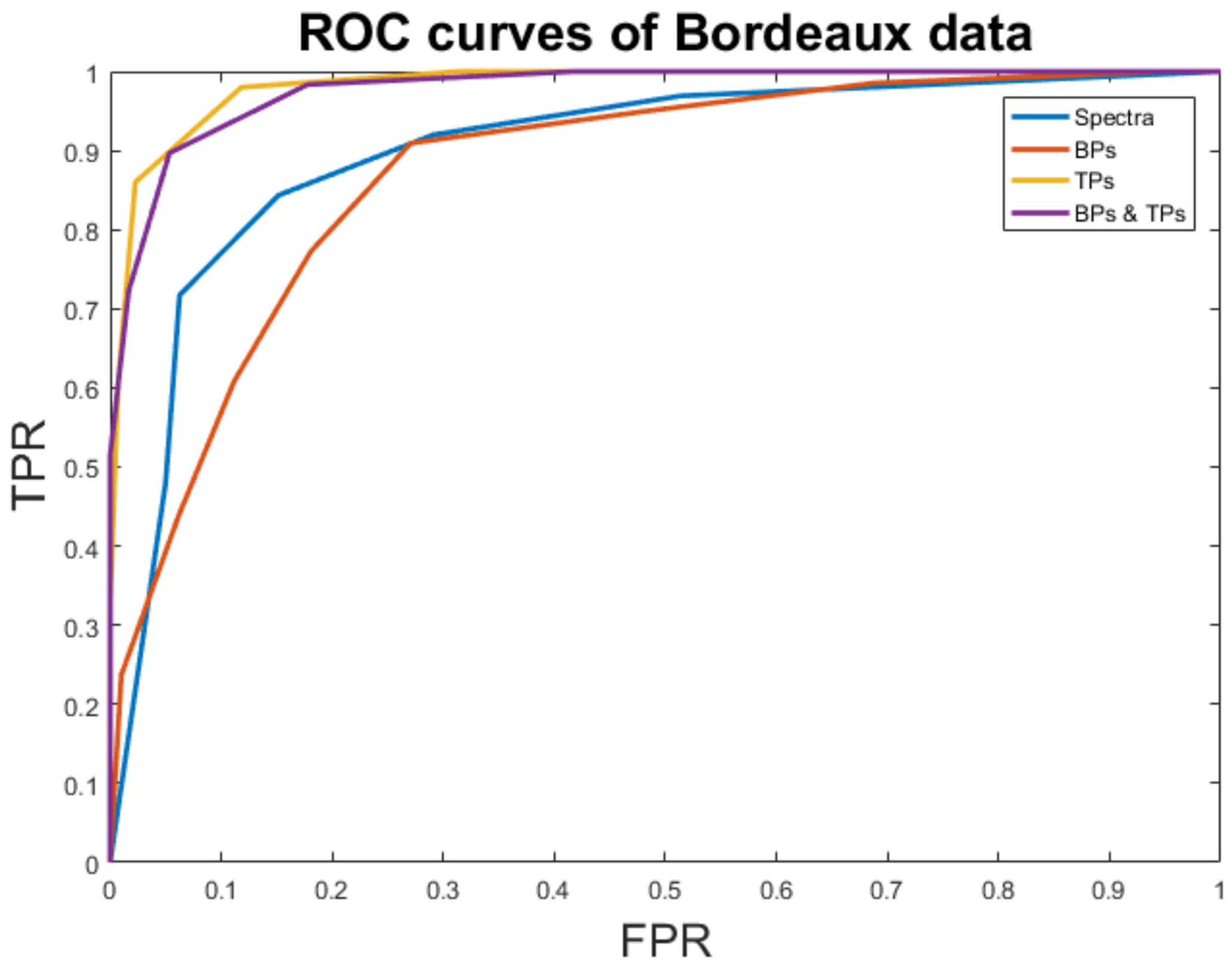
3.2.1. Classification of Esca Disease

Table 3 and Figure 9 present the classification results of data gathered from Bordeaux and the ROC curves relative for each dataset, respectively. Texture features gave the best accuracy of classification (100%). Image data were clearly more advantageous than using spectral information for the classification of Esca, in fact, when complete spectral data or BPs are applied as input, the accuracy was lower (80.62−77.5%).
Combining BPs and TPs gave a satisfying result (99.37%), implying the convenience of the association of different types of features for a better classification result.
When we evaluated the confusion matrices, we found that the number of FP and FN are almost the same, which indicates that the classifier is not over evaluating the diseased class over the healthy one.

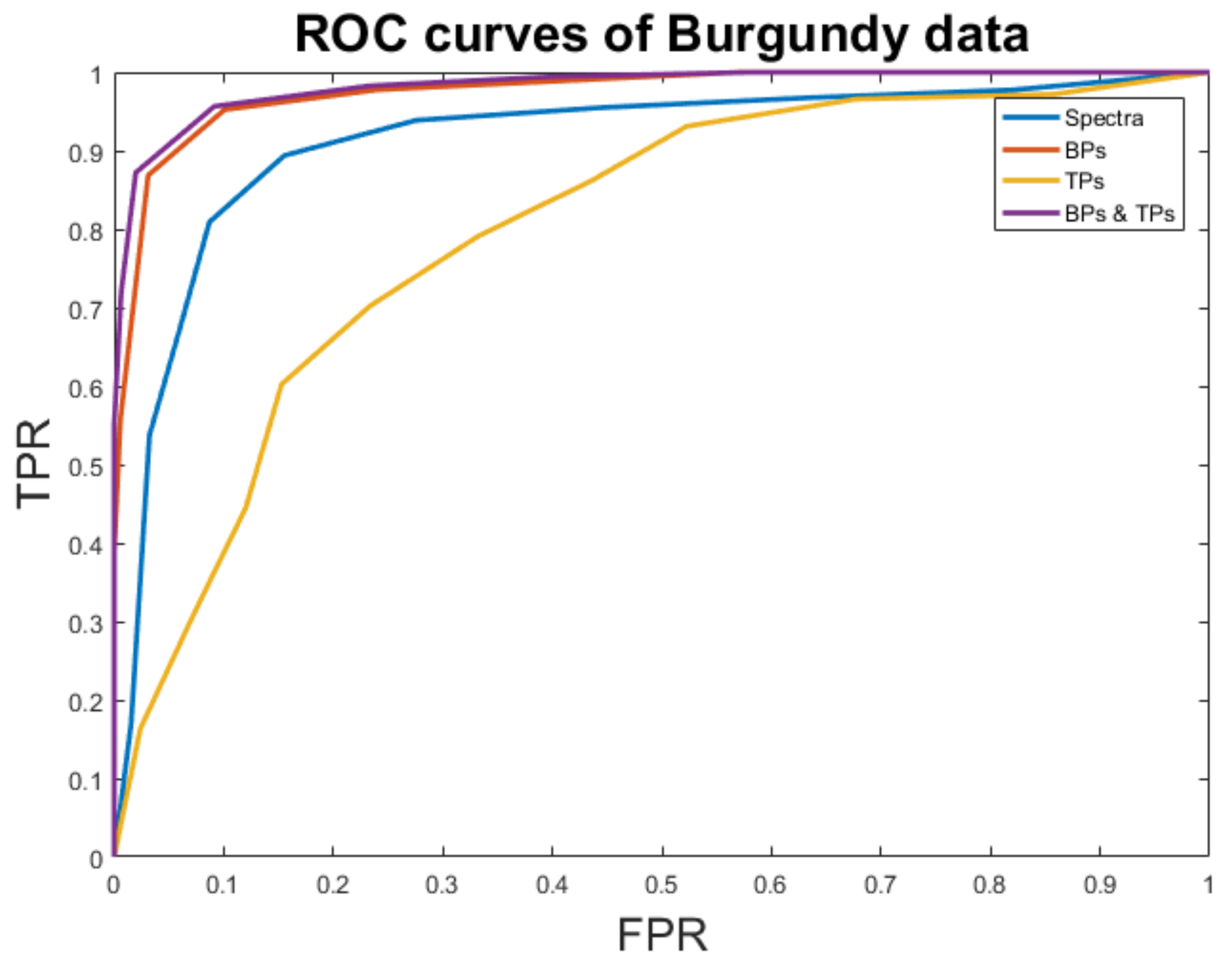
3.2.2. Classification of Yellowing Disease

Table 4 and Figure 10 present the classification results of data that were collected from Burgundy and the ROC curves relative for each dataset, respectively. For identifying the Yellowing of the grapevine, the combination of BPs and TPs gave the most accurate result of detection (99.54%). Spectral information was more adequate in this case than image data, in fact, when applying complete spectra or only BPs, the detection precision is high (93‒95.45%) with respect to only 70.45% of good results for TPs.
Similar to results that were obtained for Esca disease, we found that the classifier could present the good accordance with the truth data without over-evaluation.

4. Discussion

When comparing spectral signatures of healthy and infected red/white berried leaves in Figure 11, obvious differences can be depicted, suggesting that the spectral response was affected by the infestation. These differences come to prove the robustness of the PROSPECT model inversion that is applied in this work.
The generation of a LUT for PROSPECT model inversion is time consuming and requires extensive computation. Furthermore, it does not represent all possible cases. On the other hand, the ANN technique requires creating another model that predicts the biophysical parameters and it is exposed to a risk of over or under fitting. The PROSPECT model is already an approximation, hence, the errors are cumulated with those due to the ANN. In summary, an optimization approach seems to be the most suitable for achieving a good PROSPECT inversion. Authors in [43] identified Powell’s and Quasi-Newton iterative methods as unstable. In fact, they are unconstrained methods and they use variables without any ranges of values. In order to obtain good results [23], parameters must have good initial values and a defined range [29].
Previous studies show that there is an interaction between parameters that are inter-dependent [21,29]. Therefore, it is not feasible to combine different minimization methods together. Another solution might be to apply all of the inversion methods proposed (associated to RMSE function) simultaneously for the same reflectance spectra and choose the method that predicts the best each parameter. This will only improve the inversion model by 2%.
We tested in this study the feasibility of combining different methods and functions for the PROPSECT model inversion. None of the method-function associations were able to perfectly predict all of the parameters. As a matter of fact, the variable Car of the PROSPECT model was weakly estimated in all cases. Constrained methods were in general more relevant than unconstrained ones, but their performances are dependent on the function used. SCM function is commonly applied in remote sensing to remove the difference in intensity that is caused by shadows [31]. It does not take into account the amplitude change between measured spectra and proposed spectra by the model. Spectral reflectance is seen as a distribution, subsequently, SCM proved less efficiency with respect to other functions. RMSE and SAM belong to the same variety that consider the reflectance information as a vector in a Euclidean space. SAM function gave better results than RMSE. A global accuracy of 0.21 for RMSE and 0.58 for SAM functions were obtained. RMSE is a simple spectrum comparison that does not include random dimension. However, SAM function integrates in the denominator a covariance measure. In consequence, it takes into account the statistical variability of the PROSPECT model. To our knowledge, this is the first study that evaluates the potential of the SAM function in the case of PROSPECT model inversion. Inspired by [44], we combined SAM and RMSE functions together with the unconstrained SLSQP method. This method only took 1 s to perform the inversion and brought the best results. We recommend using a combination of both functions for a PROSPECT model inversion using reflectance solely. If the transmittance information is available, then the inversion model will be more accurate [21].
Unlike Esca, the Yellowing disease of the grapevine produces somehow homogeneous discoloration of the leaf that is not easy to be detected by textural analysis. In that case, spectral data reflecting the internal constituents of leaves were more robust in detecting contamination from normal leaves. Analyzing high dimensional hyperspectral data is globally a complex and time-consuming task. Therefore, reducing the dimensionality seems crucial for many applications. We can conclude from this work that BPs extraction was successful and could replace to some extent the use of the hyperspectral data. BPs demonstrated even higher accuracy than using complete spectral data in the case of Yellowing disease (95.45% > 93.63%) with the advantage of reducing data dimensionality. Another research [29] found interest in deducing BPs from reflectance measurements to better understand the aspects of terrestrial ecosystems, because measuring them in situ and in vivo is costly. Recently, Albetis et al. [45] estimated the ability of an Unmanned Aerial Vehicle (UAV) multispectral imagery to remotely separate Flavescence Dorée symptomatic from asymptomatic hosts in four vineyards. They used the PROSPECT model, coupled with the SAIL model [46], to take into account bidirectional reflectance when deducing the BPs.
The Esca disease induces a lot of color variations within the leaves. Since, texture describes variations in the grey-levels in an image, this explains the robustness of the texture approach in distinguishing damaged cases. In our study, texture parameters made a valuable tool for foliar disease detection, this claim was supported by other studies that are found in the scientific literature. Al-Hiary et al. [7] used some of the texture features in this study and additional ones. They were associated with a BPNN classifier in order to recognize five crop disease: Early scorch, Cottony mold, ashen mold, late scorch, and tiny whiteness. The developed algorithm could successfully detect the examined diseases with a precision between 83% and 94%. Features extracted from color co-occurrence matrices were again coupled with BPNN in [47]. The method could efficiently detect ground nut leaf detection with complex background and four different diseases with 97.41% of performance. Five diseases are studied in [48]: early scorch, cottony mold, ashen mold, late scorch, and tiny whiteness. Texture statistics for each image were generated from spatial gray-level dependence matrices. The BPNN classifier performed well and successfully classified the examined diseases with a precision of around 93%. Grape plant leaf disease detection was considered in [49]. The diseases that were tested are Downy Mildew, Powdery Mildew, and Black rot. In this work, instead of using co-occurrence texture based features, a fractal approach was applied and united to a multiclass Support Vector Machine (SVM) classifier. The proposed approach avails advice of agricultural experts easily to farmers with the accuracy of 96.6%.
At the end, we can say that depending on the disease and the type of the grapevine, the image features or the spectral features can be very useful. For Esca disease on a red-berried variety, for example, texture parameters gave excellent results, while, for Yellowing disease on a white-berried variety, spectral parameters offered more successful results. For both cases, combining both BPs and TPs gave promising accuracies (99.37‒99.54%). This work demonstrates that the combination of RGB images with hyperspectral data might be optimal for foliar disease identification. This finding is in accordance with, [50], who merged texture image analysis and spectral reflectance data to quantify damage by greenbugs for winter wheat. They found that digitally estimated, as well as visually assessed, damage by greenbugs correlated well with vegetation indices computed from reflectance data.

5. Conclusions and Perspectives

New systems are needed to respond to the worldwide spread of crop diseases. In particular, non-contact systems are required to aid farmers and producers in automatically identifying initial symptoms of plant diseases.
PROSPECT-5 was upgraded in the visible region to take into account anthocyanin (PROSPECT-D). In our inversion method, the least accurately predicted parameter was Car. An addition of another parameter to PROSPECT-5 may provide an overall increase of the inversion method precision. In the case of Grapevine that is affected by Esca showing red/brown tones, the presence of the disease might be predicted by anthocyanin pigments, therefore the PROSPECT-D model is examined for detecting Esca and Yellowing in the near future.
This study indicated that remotely sensed data that are recorded by a hyperspectral spectrometer and a digital camera have the potential to aid in monitoring damage in grapevines under field conditions. Digital image processing may offer an alternative to traditional techniques, it is advantageous because images can be reproduced, stored, and used at a later time as historical documents of vegetation status. Good results in classifying damaged leaves by biophysical parameters suggest that BPs include the dimensionality reduction of hyperspectral data and the efficiency of computation and processing. Hyperspectral imaging sensors can be used as a quick, nondestructive, repeatable, and cost-effective technique to detect Esca, Yellowing, and other types of damage in grapevines. This study was the first step to use reflectance measurements along with digital image analysis to estimate damage by Yellowing on Chardonnay grapevines and Esca on Cabernet Sauvignon grapevines. More studies are needed on other grapevine varieties and other types of diseases or stresses in order to confirm the results that were found.

Acknowledgments

We thank all the vine-growers who participated in this study that is part of the DAMAV project (Automatic Detection of Grapevine Diseases). We also would like to thank Alice Dubois and Sylvain Bernard from the Regional Federation of Defense against Pests of Provence Alpes Côtes Azur, Corinne Trarieux from the Interprofessional Office of Burgundy Wine, Jocelyn Dureuil from the Chamber of Agriculture 71 and finally Arnaud Delaherche from Pape Clement Castle in Bordeaux, for their excellent technical assistance.

Author Contributions

A.L. with the help of B.B. tested different methods and functions for the PROSPECT model inversion. A.L. implemented the spectral data analysis while H.A.-S. implemented the texture analysis of the image data and the classification technique. H.A.-S together with A.L. analyzed, discussed the results and wrote the article. The manuscript was then corrected by F.C.

Conflicts of Interest

The authors declare no conflict of interest.

References

  1. Lehrer, A.T.; Moore, P.H.; Komor, E. Impact of sugarcane yellow leaf virus (ScYLV) on the carbohydrate status of sugarcane: Comparison of virus-free plants with symptomatic and asymptomatic virus-infected plants. Physiol. Mol. Plant Pathol. 2007, 70, 180–188. [Google Scholar] [CrossRef]
  2. Matthews, R.E.F.; Hull, R.; Matthews, R.E.F. Matthews’ Plant Virology; Academic Press: San Diego, CA, USA, 2002; ISBN 978-0-08-053599-9. [Google Scholar]
  3. Mahlein, A.-K.; Steiner, U.; Dehne, H.-W.; Oerke, E.-C. Spectral signatures of sugar beet leaves for the detection and differentiation of diseases. Precis. Agric. 2010, 11, 413–431. [Google Scholar] [CrossRef]
  4. Gazala, I.F.S.; Sahoo, R.N.; Pandey, R.; Mandal, B.; Gupta, V.K.; Singh, R.; Sinha, P. Spectral reflectance pattern in soybean for assessing yellow mosaic disease. Indian J. Virol. 2013, 24, 242–249. [Google Scholar] [CrossRef] [PubMed]
  5. Huang, J.; Liao, H.; Zhu, Y.; Sun, J.; Sun, Q.; Liu, X. Hyperspectral detection of rice damaged by rice leaf folder (Cnaphalocrocis medinalis). Comput. Electron. Agric. 2012, 82, 100–107. [Google Scholar] [CrossRef]
  6. Atzberger, C.; Darvishzadeh, R.; Immitzer, M.; Schlerf, M.; Skidmore, A.; le Maire, G. Comparative analysis of different retrieval methods for mapping grassland leaf area index using airborne imaging spectroscopy. Int. J. Appl. Earth Obs. Geoinf. 2015, 43, 19–31. [Google Scholar] [CrossRef]
  7. Al-Hiary, H.; Bani-Ahmad, S.; Reyalat, M.; Braik, M.; ALRahamneh, Z. Fast and accurate detection and classification of plant diseases. Mach. Learn. 2011, 14, 31–38. [Google Scholar] [CrossRef]
  8. Camargo, A.; Smith, J.S. Image pattern classification for the identification of disease causing agents in plants. Comput. Electron. Agric. 2009, 66, 121–125. [Google Scholar] [CrossRef]
  9. Majumdar, D.; Kole, D.K.; Chakraborty, A.; Dutta, D. Detection and diagnosis of plant leaf disease using integrated image processing approach. Int. J. Comput. Eng. Appl. 2014, 6, 10–16. [Google Scholar]
  10. Xie, C.; He, Y. Spectrum and Image Texture Features Analysis for Early Blight Disease Detection on Eggplant Leaves. Sensors 2016, 16, 676. [Google Scholar] [CrossRef] [PubMed]
  11. Xie, C.; Shao, Y.; Li, X.; He, Y. Detection of early blight and late blight diseases on tomato leaves using hyperspectral imaging. Sci. Rep. 2015, 5. [Google Scholar] [CrossRef] [PubMed]
  12. Carisse, O.; Canada, Agriculture and Agri-Food Canada, Québec (Province); Ministère de l’agriculture, des pêcheries et de l’alimentation. Identification Guide to the Major Diseases of Grapes; Agriculture and Agri-Food Canada: Ottawa, ON, Canada, 2006; ISBN 978-0-662-43594-5.
  13. Li, S.; Bonneu, F.; Chadoeuf, J.; Picart, D.; Gégout-Petit, A.; Guérin-Dubrana, L. Spatial and Temporal Pattern Analyses of Esca Grapevine Disease in Vineyards in France. Phytopathology 2017, 107, 59–69. [Google Scholar] [CrossRef] [PubMed]
  14. Lecomte, P.; Darrieutort, G.; Liminana, J.-M.; Comont, G.; Muruamendiaraz, A.; Legorburu, F.-J.; Choueiri, E.; Jreijiri, F.; El Amil, R.; Fermaud, M. New insights into esca of grapevine: The development of foliar symptoms and their association with xylem discoloration. Plant Dis. 2012, 96, 924–934. [Google Scholar] [CrossRef]
  15. Grapevine Measles. Available online: http://articles.extension.org/pages/64365/grapevine-measles (accessed on 6 March 2018).
  16. Esca (Black Measles). Available online: http://ipm.ucanr.edu/PMG/r302100511.html (accessed on 15 March 2018).
  17. Mugnai, L.; Graniti, A.; Surico, G. Esca (black measles) and brown wood-streaking: two old and elusive diseases of grapevines. Plant Dis. 1999, 83, 404–418. [Google Scholar] [CrossRef]
  18. Grapevine Yellows Information—Is There A Treatment For Grapevine Yellows. Available online: https://www.gardeningknowhow.com/edible/fruits/grapes/grapevine-yellows-information.htm (accessed on 27 March 2018).
  19. Chuche, J.; Thiéry, D. Biology and ecology of the Flavescence dorée vector Scaphoideus titanus: A review. Agron. Sustain. Dev. 2014, 34, 381–403. [Google Scholar] [CrossRef]
  20. Jacquemoud, S.; Baret, F. PROSPECT: A model of leaf optical properties spectra. Remote Sens. Environ. 1990, 34, 75–91. [Google Scholar] [CrossRef]
  21. Feret, J.-B.; François, C.; Asner, G.P.; Gitelson, A.A.; Martin, R.E.; Bidel, L.P.R.; Ustin, S.L.; le Maire, G.; Jacquemoud, S. PROSPECT-4 and 5: Advances in the leaf optical properties model separating photosynthetic pigments. Remote Sens. Environ. 2008, 112, 3030–3043. [Google Scholar] [CrossRef]
  22. Darvishzadeh, R.; Skidmore, A.; Schlerf, M.; Atzberger, C. Inversion of a radiative transfer model for estimating vegetation LAI and chlorophyll in a heterogeneous grassland. Remote Sens. Environ. 2008, 112, 2592–2604. [Google Scholar] [CrossRef]
  23. Duan, S.-B.; Li, Z.-L.; Wu, H.; Tang, B.-H.; Ma, L.; Zhao, E.; Li, C. Inversion of the PROSAIL model to estimate leaf area index of maize, potato, and sunflower fields from unmanned aerial vehicle hyperspectral data. Int. J. Appl. Earth Obs. Geoinf. 2014, 26, 12–20. [Google Scholar] [CrossRef]
  24. Romero, A.; Aguado, I.; Yebra, M. Estimation of dry matter content in leaves using normalized indexes and PROSPECT model inversion. Int. J. Remote Sens. 2012, 33, 396–414. [Google Scholar] [CrossRef]
  25. Weiss, M.; Baret, F.; Myneni, R.; Pragnère, A.; Knyazikhin, Y. Investigation of a model inversion technique to estimate canopy biophysical variables from spectral and directional reflectance data. Agronomie 2000, 20, 3–22. [Google Scholar] [CrossRef]
  26. Sehgal, V.K.; Chakraborty, D.; Sahoo, R.N. Inversion of radiative transfer model for retrieval of wheat biophysical parameters from broadband reflectance measurements. Inf. Process. Agric. 2016, 3, 107–118. [Google Scholar] [CrossRef]
  27. Atzberger, C. Object-based retrieval of biophysical canopy variables using artificial neural nets and radiative transfer models. Remote Sens. Environ. 2004, 93, 53–67. [Google Scholar] [CrossRef]
  28. Berjón, A.J.; Cachorro, V.E.; Zarco-Tejada, P.J.; de Frutos, A. Retrieval of biophysical vegetation parameters using simultaneous inversion of high resolution remote sensing imagery constrained by a vegetation index. Precis. Agric. 2013, 14, 541–557. [Google Scholar] [CrossRef]
  29. Li, P.; Wang, Q. Retrieval of Leaf Biochemical Parameters Using PROSPECT Inversion: A New Approach for Alleviating Ill-Posed Problems. IEEE Trans. Geosci. Remote Sens. 2011, 49, 2499–2506. [Google Scholar] [CrossRef]
  30. Nelder, J.A.; Mead, R. A Simplex Method for Function Minimization. Comput. J. 1965, 7, 308–313. [Google Scholar] [CrossRef]
  31. Deborah, H.; Richard, N.; Hardeberg, J.Y. A Comprehensive Evaluation of Spectral Distance Functions and Metrics for Hyperspectral Image Processing. IEEE J. Sel. Top. Appl. Earth Obs. Remote Sens. 2015, 8, 3224–3234. [Google Scholar] [CrossRef]
  32. Zhu, C.; Byrd, R.; Lu, P.; Nocedal, J. LBFGS-B Fortran Subroutines for Large-Scale Bound Constrained Optimization; Report NAM-11 EECS Department, Northwestern University: Evanston, IL, USA, 31 December 1994; pp. 1–17. [Google Scholar]
  33. Sequential Quadratic Programming. Numerical Optimization; Springer: New York, NY, USA, 2006; pp. 529–562. ISBN 978-0-387-30303-1. [Google Scholar]
  34. Nash, S.G. Preconditioning of Truncated-Newton Methods. SIAM J. Sci. Stat. Comput. 1985, 6, 599–616. [Google Scholar] [CrossRef]
  35. Haralick, R.M.; Shanmugam, K.; Dinstein, I. Textural Features for Image Classification. IEEE Trans. Syst. Man Cybern. 1973, SMC-3, 610–621. [Google Scholar] [CrossRef]
  36. Pydipati, R.; Burks, T.F.; Lee, W.S. Identification of citrus disease using color texture features and discriminant analysis. Comput. Electron. Agric. 2006, 52, 49–59. [Google Scholar] [CrossRef]
  37. Arivazhagan, S.; Shebiah, R.N.; Ananthi, S.; Varthini, S.V. Detection of unhealthy region of plant leaves and classification of plant leaf diseases using texture features. Agric. Eng. Int. CIGR J. 2013, 15, 211–217. [Google Scholar]
  38. Sannakki, S.S.; Rajpurohit, V.S.; Nargund, V.B.; Kulkarni, P. Diagnosis and classification of grape leaf diseases using neural networks. In Proceedings of the 2013 Fourth International Conference on Computing, Communications and Networking Technologies (ICCCNT), Tiruchengode, India, 4–6 July 2013; pp. 1–5. [Google Scholar]
  39. Torheim, T.; Malinen, E.; Kvaal, K.; Lyng, H.; Indahl, U.G.; Andersen, E.K.F.; Futsaether, C.M. Classification of Dynamic Contrast Enhanced MR Images of Cervical Cancers Using Texture Analysis and Support Vector Machines. IEEE Trans. Med. Imaging 2014, 33, 1648–1656. [Google Scholar] [CrossRef] [PubMed]
  40. Chaddad, A.; Tanougast, C.; Dandache, A.; Bouridane, A. Extracted haralick’s texture features and morphological parameters from segmented multispectrale texture bio-images for classification of colon cancer cells. WSEAS Trans. Biol. Biomed. 2011, 8, 39–50. [Google Scholar]
  41. Rojas, R. Neural Networks: A Systematic Introduction; Springer Science & Business Media: Berlin/Heidelberg, Germany, 1996; ISBN 978-3-642-61068-4. [Google Scholar]
  42. Miller, W.M.; Drouillard, G.P. Multiple Feature Analysis for Machine Vision Grading of Florida Citrus. Appl. Eng. Agric. 2001, 17. [Google Scholar] [CrossRef]
  43. Durbha, S.S.; King, R.L.; Younan, N.H. Support vector machines regression for retrieval of leaf area index from multiangle imaging spectroradiometer. Remote Sens. Environ. 2007, 107, 348–361. [Google Scholar] [CrossRef]
  44. Price, J.C. How unique are spectral signatures? Remote Sens. Environ. 1994, 49, 181–186. [Google Scholar] [CrossRef]
  45. Albetis, J.; Duthoit, S.; Guttler, F.; Jacquin, A.; Goulard, M.; Poilvé, H.; Féret, J.-B.; Dedieu, G. Detection of Flavescence dorée Grapevine Disease Using Unmanned Aerial Vehicle (UAV) Multispectral Imagery. Remote Sens. 2017, 9, 308. [Google Scholar] [CrossRef]
  46. Verhoef, W. Light scattering by leaf layers with application to canopy reflectance modeling: the SAIL model. Remote Sens. Environ. 1984, 16, 125–141. [Google Scholar] [CrossRef]
  47. Ramakrishnan, M. Groundnut leaf disease detection and classification by using back probagation algorithm. In Proceedings of the Communications and Signal Processing (ICCSP), Melmaruvathur, India, 2–4 April 2015; pp. 0964–0968. [Google Scholar]
  48. Al Bashish, D.; Braik, M.; Bani-Ahmad, S. Detection and Classification of Leaf Diseases using K-means-based Segmentation and Neural-networks-based Classification. Inf. Technol. J. 2011, 10, 267–275. [Google Scholar] [CrossRef]
  49. Waghmare, H.; Kokare, R.; Dandawate, Y. Detection and classification of diseases of Grape plant using opposite colour Local Binary Pattern feature and machine learning for automated Decision Support System. In Proceedings of the Signal Processing and Integrated Networks (SPIN), Noida, India, 11–12 February 2016; pp. 513–518. [Google Scholar]
  50. Mirik, M.; Michels, G.J.; Kassymzhanova-Mirik, S.; Elliott, N.C.; Catana, V.; Jones, D.B.; Bowling, R. Using digital image analysis and spectral reflectance data to quantify damage by greenbug (Hemitera: Aphididae) in winter wheat. Comput. Electron. Agric. 2006, 51, 86–98. [Google Scholar] [CrossRef]
Figure 1. Symptoms of Esca on Cabernet Sauvignon grapevines in Aquitaine region, France.
Remotesensing 10 00618 g001
Figure 2. Symptoms of Yellowing on Chardonnay grapevines in Burgundy region, France.
Remotesensing 10 00618 g002
Figure 3. Map showing French wine growing regions. Studied regions are Burgundy and Bordeaux (green ellipses).
Remotesensing 10 00618 g003
Figure 4. Locations of the measurements on a sample leaf.
Remotesensing 10 00618 g004
Figure 5. Example of Red Green Blue (RGB) image taken on a healthy Grenache leaf.
Remotesensing 10 00618 g005
Figure 6. Flowchart of the methodology used for disease detection. (Abbreviations in the figure are: Red Green Blue (RGB), Inversion Method (IM), Sequential Least Squares Programming (SLSQP), Function Method (FM), Root Mean Square Error (RMSE), and Spectral Angle Mapper (SAM)).
Remotesensing 10 00618 g006
Figure 7. Workflow to compare real and predicted values of biophysical parameters each method and function. X combinations were defined to 221,184 in this study.
Remotesensing 10 00618 g007
Figure 8. Pre-processing of the RGB digital images (Red-Green-Blue (RGB), Hue-Saturation-Value (HSV)).
Remotesensing 10 00618 g008
Figure 9. ROC curves of Esca disease classification with Back Propagation Neural Networks (BPNN) when hyperspectral data is used, biophysical parameters, texture parameters and combined biophysical and texture parameters. Horizontal and vertical axes are TPR and FPR, respectively. (Receiver Operating Characteristic (ROC), True Positive Rate (TPR), and False Positive Rate (FPR)).
Remotesensing 10 00618 g009
Figure 10. ROC curves of Yellowing disease with BPNN when hyperspectral data is used, biophysical parameters, texture parameters, and combined biophysical and texture parameters. Horizontal and vertical axes are TPR and FPR, respectively. (Receiver Operating Characteristic (ROC), True Positive Rate (TPR), False Positive Rate (FPR)).
Remotesensing 10 00618 g010
Figure 11. Spectral reflectance corresponding to the average of healthy (green) and infected (red) leaf groups. (a) correspond to Cabernet Sauvignon variety infected by Esca; and (b) corresponds to Chardonnay variety infected by Yellowing.
Remotesensing 10 00618 g011
Table 1. Range considered for each biophysical parameter.
ParametersAbbreviationUnitMinMaxStep
Leaf structure coefficientNNo dimension0.53.50.5
Leaf chlorophyll contentCabμg/cm20.000011200.5
Leaf carotenoid contentCarμg/cm20.00001300.5
Brown pigment contentCbrownArbitrary units0.000010.80.1
Equivalent water thicknessCwcm0.000010.080.01
Dry matter contentCmg/cm20.000010.040.01
Table 2. Results of R-squared values from different methods and functions of PROSPECT inversion. In bold, the higher R-squared values for the selected method and function. The underlined values refer to higher R-squared values for each other functions.
MethodsFunctionNCabCarCbrownCwCmGlobal Accuracy
L-BFGS-BRMSE0.97060.86360.46730.72930.90900.84470.2193
SLSQP0.96940.72850.30820.72930.94830.70440.1060
TNC0.87650.67310.43600.52010.93800.50680.0636
Nelder-Mead0.02380.02680.02190.02900.01170.03630.0000
L-BFGS-BSCM0.26710.48260.25020.77190.84050.56600.0118
SLSQP0.03660.11660.03310.50810.51900.16230.0000
TNC0.23420.48440.24180.58170.76770.49840.0061
Nelder-Mead0.00940.03660.04650.04460.04830.02130.0000
L-BFGS-BSAM0.70060.78570.55970.83720.98530.89530.2275
SLSQP0.97420.99160.61860.99440.99640.98720.5845
TNC0.17460.32940.11320.29920.75500.35400.0005
Nelder-Mead0.00320.03160.02660.00660.05160.01980.0000
L-BFGS-BSAM + RMSE0.97420.65380.54850.75100.76040.78320.1563
SLSQP0.99960.99520.68740.99380.99860.99620.6761
TNC0.73030.37970.06870.19130.86160.33870.0011
Nelder-Mead0.01690.02840.02060.02650.03910.01350.0000
Table 3. Classification of Esca disease based on complete spectra, BPs and TPs. (Biophysical Parameters (BPs), Texture Parameters (TPs)).
AccuracyFMAUC
Spectra80.62%0.780.90
BPs77.50%0.670.82
TPs100%10.98
BPs + TPs99.37%0.990.97
Table 4. Classification of Yellowing disease based on complete spectra, BPs and TPs. (Biophysical Parameters (BPs), Texture Parameters (TPs), F-Measure (FM), Area Under ROC (AUC)).
AccuracyFMAUC
Spectra93.63%0.920.91
BPs95.45%0.950.97
TPs70.45%0.690.80
BPs + TPs99.54%0.990.98

