Surveying Drifting Icebergs and Ice Islands: Deterioration Detection and Mass Estimation with Aerial Photogrammetry and Laser Scanning


Abstract

1. Introduction
2. Field Methods
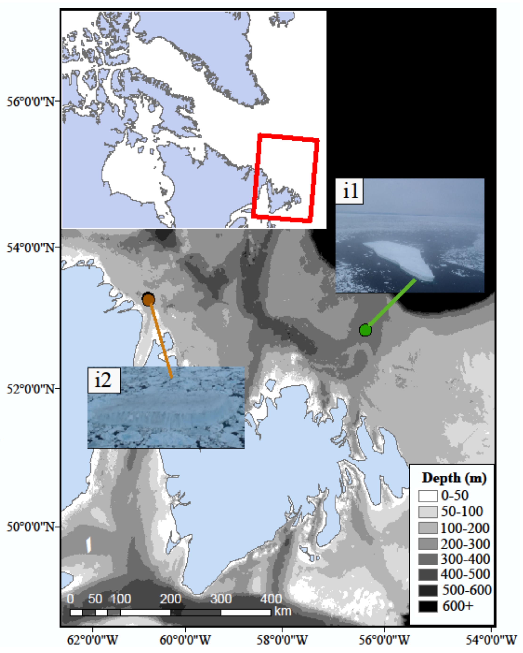
2.1. Field Setting
2.2. Marker/GPS Deployment
2.3. Aerial Photography Surveying
2.4. Terrestrial Laser Scan Surveying
3. Analysis Methods
3.1. Point Cloud Processing
3.1.1. Structure-from-Motion Photogrammetry
3.1.2. Terrestrial Laser Scanning
3.2. Point Cloud Comparison and DDT Calculation
3.2.1. The Multiscale Model-to-Model Cloud Comparison Algorithm
3.2.2. Structure-from-Motion Photogrammetry Derived Point Clouds
3.2.3. Terrestrial Laser Scanning Point Clouds
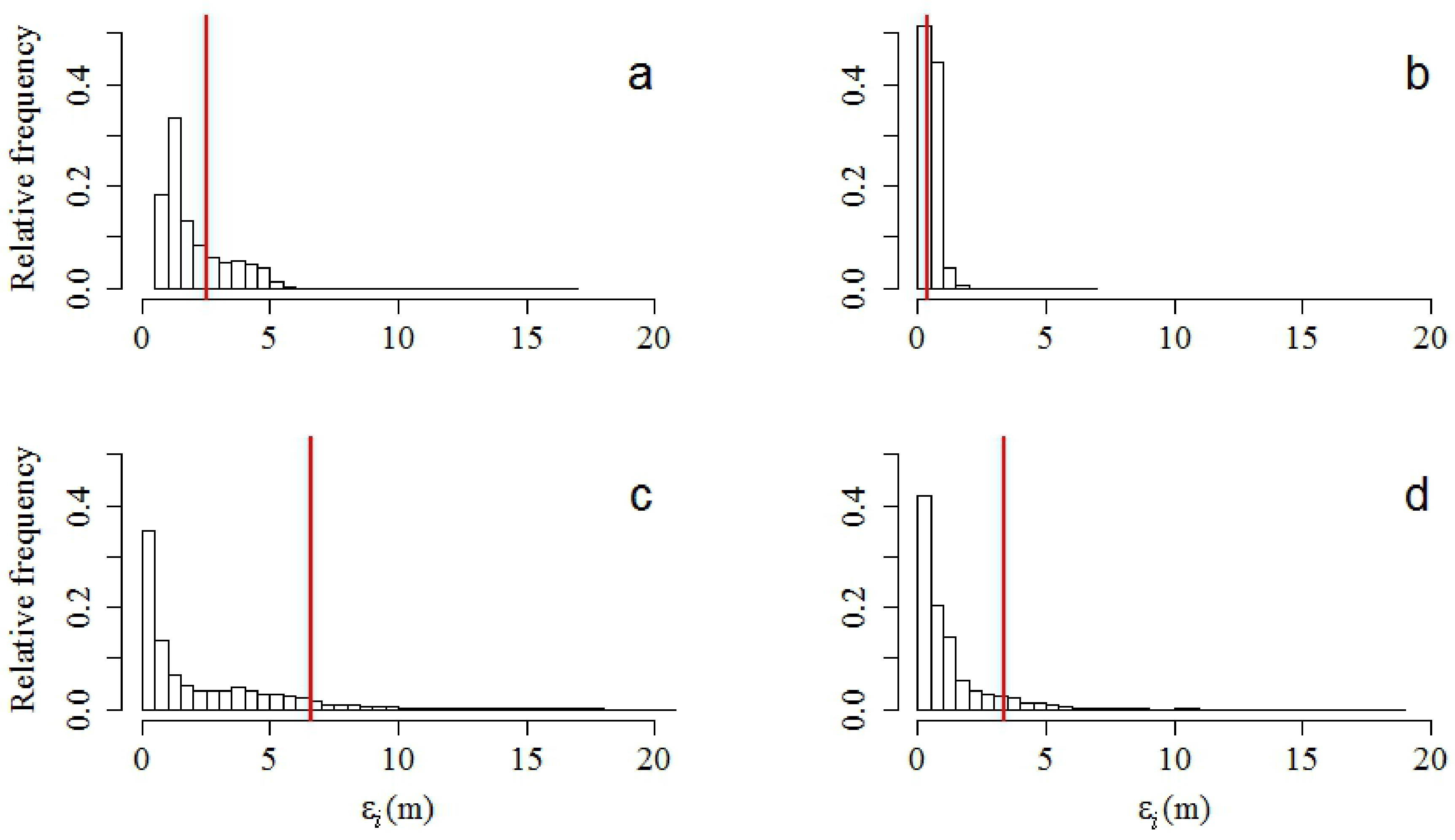
3.2.4. Deterioration Detection Threshold Computation
3.3. Mass Estimation
4. Results
4.1. Iceberg Characteristics and Mass Estimation
4.2. Survey Quality and DDT Values
4.2.1. Aerial Photography with SfM Processing
4.2.2. Terrestrial Laser Scan Surveying
4.3. Beacon Data
5. Discussion
5.1. Data Collection and Processing Considerations
5.1.1. Detection Thresholds and Monitoring Iceberg Deterioration Processes
5.1.2. M3C2 Algorithm
5.2. Comparison to Previous Work and Recommendations
5.2.1. Deterioration Detection and Mass Estimation
5.2.2. Surveying Workflows
5.2.3. Future Iceberg and Ice Island Surveying
6. Conclusions
Supplementary Materials
Acknowledgments
Author Contributions
Conflicts of Interest
Abbreviations
| A | Area |
| AUV | Automated underwater vehicle |
| d | Distance |
| dx,dy | Distance in x and y dimensions |
| D | Diameter used for surface normal calculation |
| DDT | Deterioration detection threshold |
| DEM | Digital elevation model |
| f | Freeboard |
| GCP | Ground control point |
| GNSS | Global navigation satellite system |
| GPS | Global positioning system |
| hGPS | GPS heading |
| hOFF | Heading offset between hGPS and hpc |
| hpc | Cloud point to GPS heading |
| i1, i2 | ‘iceberg-1’, ‘iceberg-2’ |
| IBRF | Iceberg reference frame |
| inter-GCP distance | Euclidean distance between GCPs; used for scale assignment in SfM processing |
| ISE | Inter-survey error |
| IMU | Inertial measurement unit |
| INS | Inertial navigation system |
| L | Length |
| M | Mass |
| M3C2 | Multiscale Model-to-Model Cloud Comparison [algorithm] |
| N | Surface normal |
| n | Number of points within a projected cylinder used during the M3C2 algorithm |
| p | Diameter used for M3C2 projection cylinder |
| PCdist-i | Distance calculated between point clouds at core point ‘i’ with M3C2 |
| PPP | Precise point positioning |
| SfM | Structure-from-motion multi-view stereo photogrammetry |
| SPAN | Synchronous position, attitude and navigation |
| TLS | Terrestrial laser scanning |
| ui | Uncertainty associated with each PCdist-i value output from M3C2 |
| UAV | Unmanned aerial vehicle |
| UTM | Universal Transverse Mercator |
| V | Volume |
| W | Width |
| δ | Maximum search distance used in M3C2 |
| ξ | Normal scale assessment criterion |
| εi | Total error at each core point |
| σ | Standard deviation |
| σbx, σby, σbz | Standard deviation of beacon position in the x-, y-, and z-planes |
| σi | Surface roughness around core point ‘i’ |
| σ1i, σ2i | Surface roughness around core point ‘i’ for reference and compared point clouds |
| ρp | Point density (points m−2) |
| ρi | Ice density (873 kg m−3) |
| ρw | Water density (1025 kg m−3) |
References
- Crawford, A.; Crocker, G.; Desjardins, L.; Saper, R.; Mueller, D. The Canadian Ice Island Drift Deterioration and Detection (CI2D3) Database. J. Glaciol. 2017. (In Press)
- Hogg, A.; Gudmundsson, G.H. Impacts of the Larsen-C Ice Shelf calving event. Nat. Clim. Chang. 2017, 7, 540–542. [Google Scholar] [CrossRef]
- Allison, K.; Crocker, G.; Tran, H.; Carrieres, T. An ensemble forecast model of iceberg drift. Cold Reg. Sci. Technol. 2014, 108, 1–9. [Google Scholar] [CrossRef]
- Crocker, G.; Carrieres, T.; Tran, H. Ice island drift and deterioration forecasting in eastern Canada. In Proceedings of the 22nd International Conference on Port and Ocean Engineering Under Arctic Conditions, Espoo, Finland, 9–13 June 2013. [Google Scholar]
- Fuglem, M.; Jordaan, I. Risk analysis and hazards of ice islands. In Arctic Ice Shelves and Ice Islands; Copland, L., Mueller, D., Eds.; Springer: Dordrecht, The Netherlands, 2017; pp. 395–415. [Google Scholar] [CrossRef]
- Kubat, I.; Sayed, M.; Savage, S.B.; Carrieres, T.; Crocker, G. An operational iceberg deterioration model. In Proceedings of the 17th International Society of Offshore and Polar Engineers, Lisbon, Portugal, 1–6 July 2007; International Society of Offshore and Polar Engineers (ISOPE): Cupertino, CL, USA, 2007; pp. 652–657. [Google Scholar]
- Kubat, I.; Sayed, M.; Savage, S.B.; Carrieres, T. An operational model of iceberg drift. Int. J. Offshore Polar Eng. 2005, 15, 125–131. [Google Scholar]
- Gladstone, R.M.; Bigg, G.R.; Nicholls, K.W. Iceberg trajectory modeling and meltwater injection in the Southern Ocean. J. Geophys. Res. 2001, 106, 19903–19915. [Google Scholar] [CrossRef]
- Kimball, P.W.; Rock, S.M. Mapping of translating, rotating icebergs with an autonomous underwater vehicle. IEEE J. Ocean. Eng. 2015, 40, 196–208. [Google Scholar] [CrossRef]
- Merino, N.; Le Sommer, J.; Durand, G.; Jourdain, N.C.; Madec, G.; Mathiot, P.; Tournadre, J. Antarctic icebergs melt over the Southern Ocean: Climatology and impact on sea ice. Ocean Model. 2016, 104, 99–110. [Google Scholar] [CrossRef]
- Smith, K.L.; Sherman, A.D.; Shaw, T.J.; Sprintall, J. Icebergs as unique Lagrangian ecosystems in Polar Seas. Annu. Rev. Mar. Sci. 2013, 5, 269–287. [Google Scholar] [CrossRef] [PubMed]
- Enderlin, E.M.; Hamilton, G.S. Estimates of iceberg submarine melting from high-resolution digital elevation models: Application to Sermilik Fjord, East Greenland. J. Glaciol. 2014, 60, 1084–1092. [Google Scholar] [CrossRef]
- Enderlin, E.M.; Hamilton, G.S.; Straneo, F.; Sutherland, D.A. Iceberg meltwater fluxes dominate the freshwater budget in Greenland’s iceberg-congested glacial fjords. Geophys. Res. Lett. 2016, 43. [Google Scholar] [CrossRef]
- Hamilton, A.K.; Forrest, A.L.; Crawford, A.; Schmidt, V.; Laval, B.E.; Mueller, D.R.; Brucker, S.; Hamilton, T. Project ICEBERGS Final Report to Environment Canada; Canadian Ice Service, Environment Canada: Ottawa, ON, Canada, 2013; p. 36.
- Saper, R.; Tivy, A.; Mueller, D.; Nacke, M. Report of the Inaugural Meeting of the Glacial Ice Hazards Working Group (GIHWG); Carleton University: Ottawa, ON, Canada, 2015; p. 30. [Google Scholar]
- Crawford, A.; Mueller, D.R.; Humphreys, E.; Carrieres, T.; Tran, H. Surface ablation model evaluation on a drifting ice island in the Canadian Arctic. Cold Reg. Sci. Technol. 2015, 110, 170–182. [Google Scholar] [CrossRef]
- McGill, P.R.; Reisenbichler, K.R.; Etchemendy, S.A.; Dawe, T.C.; Hobson, B.W. Aerial surveys and tagging of free-drifting icebergs using an unmanned aerial vehicle (UAV). Deep Sea Res. Part II Top. Stud. Oceanogr. 2011, 58, 1318–1326. [Google Scholar] [CrossRef]
- Kimball, P.; Rock, S. Sonar-based iceberg-relative navigation for autonomous underwater vehicles. Deep Sea Res. Part II Top. Stud. Oceanogr. 2011, 58, 1301–1310. [Google Scholar] [CrossRef]
- Fonstad, M.A.; Dietrich, J.T.; Courville, B.C.; Jensen, J.L.; Carbonneau, P.E. Topographic structure from motion: A new development in photogrammetric measurement. Earth Surf. Process. Landf. 2013, 38, 421–430. [Google Scholar] [CrossRef]
- Quan, L. Image-Based Modeling; Springer: New York, NY, USA, 2010. [Google Scholar]
- Westoby, M.J.; Brasington, J.; Glasser, N.F.; Hambrey, M.J.; Reynolds, J.M. ‘Structure-from-motion’ photogrammetry: A low-cost, effective tool for geoscience applications. Geomorphology 2012, 179, 300–314. [Google Scholar] [CrossRef]
- Snavely, N.; Simon, I.; Goesele, M.; Szeliski, R.; Seitz, S.M. Scene reconstruction and visualization from community photo collections. Proc. IEEE 2010, 98, 1370–1390. [Google Scholar] [CrossRef]
- Thomson, L.; Copland, L. White Glacier 2014, Axel Heiberg Island, Nunavut: Mapped using structure from motion methods. J. Maps 2016, 1063–1071. [Google Scholar] [CrossRef]
- Javernick, L.; Brasington, J.; Caruso, B. Modeling the topography of shallow braided rivers using structure-from-motion photogrammetry. Geomorphology 2014, 213, 166–182. [Google Scholar] [CrossRef]
- Girod, L.; Nuth, C.; Kääb, A.; Etzelmüller, B.; Kohler, J. Terrain changes from images acquired on opportunistic flights by SfM photogrammetry. Cryosphere 2017, 11, 827–840. [Google Scholar] [CrossRef]
- Aber, J.S.; Marzolff, I.; Ries, J.B. Small-Format Aerial Photography: Principles, Techniques and Geoscience Applications, 1st ed.; Elsevier: Amsterdam, The Netherlands, 2010; p. 266. [Google Scholar]
- Whitehead, K.; Moorman, B.J.; Hugenholtz, C.H. Brief communication: Low-cost, on-demand aerial photogrammetry for glaciological measurement. Cryosphere 2013, 7, 1879–1884. [Google Scholar] [CrossRef]
- Beedle, M.J.; Menounos, B.; Wheate, R. An evaluation of mass-balance methods applied to Castle Creek Glacier, British Columbia, Canada. J. Glaciol. 2014, 60, 262–276. [Google Scholar] [CrossRef]
- Brun, F.; Buri, P.; Miles, E.S.; Wagnon, P.; Steiner, J.; Berthier, E.; Ragettli, S.; Kraaijenbrink, P.; Immerzeel, W.W.; Pellicciotti, F. Quantifying volume loss from ice cliffs on debris-covered glaciers using high-resolution terrestrial and aerial photogrammetry. J. Glaciol. 2016, 684–695. [Google Scholar] [CrossRef]
- Ryan, J.C.; Hubbard, A.L.; Box, J.E.; Todd, J.; Christoffersen, P.; Carr, J.R.; Holt, T.O.; Snooke, N. UAV photogrammetry and structure from motion to assess calving dynamics at Store Glacier, a large outlet draining the Greenland ice sheet. Cryosphere 2015, 9, 1–11. [Google Scholar] [CrossRef]
- Divine, D.V.; Pedersen, C.A.; Karlsen, T.I.; Aas, H.F.; Granskog, M.A.; Hudson, S.R.; Gerland, S. Photogrammetric retrieval and analysis of small scale sea ice topography during summer melt. Cold Reg. Sci. Technol. 2016, 129, 77–84. [Google Scholar] [CrossRef]
- Younan, A.; Ralph, F.; Ralph, T.; Bruce, J. Overview of the 2012 Iceberg Profiling Program. In Proceedings of the Offshore Technology Conference, St. John’s, NL, Canada, 24–26 October 2016. [Google Scholar] [CrossRef]
- Robe, R.Q.; Farmer, L.D. Part I. Height to draft ratios of icebergs; Part II. Mass estimation of Arctic icebergs. In Physical Properties of Icebergs; Department of Transportation, United States Coast Guard: Washington, DC, USA, 1976; p. 26. [Google Scholar]
- Cook, S.; Rutt, I.C.; Murray, T.; Luckman, A.; Zwinger, T.; Selmes, N.; Goldsack, A.; James, T.D. Modelling environmental influences on calving at Helheim Glacier in eastern Greenland. Cryosphere 2014, 8, 827–841. [Google Scholar] [CrossRef]
- Landy, J.C.; Isleifson, D.; Komarov, A.S.; Barber, D.G. Parameterization of centimeter-scale sea ice surface roughness using terrestrial LiDAR. IEEE Trans. Geosci. Remote Sens. 2015, 53, 1271–1286. [Google Scholar] [CrossRef]
- Kamintzis, J.E.; Jones, J.P.P.; Irvine-Fynn, T.D.L.; Holt, T.O.; Bunting, P.; Jennings, S.J.A.; Porter, P.R.; Hubbard, B. Assessing the applicability of terrestrial laser scanning for mapping englacial conduits. J. Glaciol. 2018, 24, 37–48. [Google Scholar] [CrossRef]
- Eisen, B. Acoustic Mapping of a Moving Iceberg in the Canadian Arctic. Bachelor’s Thesis, University of New Brunswick, Fredricton, NB, Canada, 2012; p. 69. [Google Scholar]
- Forrest, A.L.; Hamilton, A.K.; Schmidt, V.E.; Laval, B.E.; Mueller, D.R.; Crawford, A.; Brucker, S.; Hamilton, T. Digital terrain mapping of Petermann Ice Island fragments in the Canadian High Arctic. In Proceedings of the 21st IAHR International Symposium on Ice, Dalian, China, 11–15 June 2012; pp. 710–721. [Google Scholar]
- McGuire, P.; Younan, A.; Wang, Y.; Bruce, J.; Gandi, M.; King, T.; Keeping, K.; Regular, K. Smart Iceberg Management System—rapid iceberg profiling system. In Proceedings of the Offshore Technology Conference, St. John’s, NL, Canada, 24–26 October 2016; pp. 1706–1712. [Google Scholar] [CrossRef]
- Wagner, T.J.W.; Wadhams, P.; Bates, R.; Elosegui, P.; Stern, A.; Vella, D.; Abrahamsen, E.P.; Crawford, A.; Nicholls, K.W. The “footloose” mechanism: Iceberg decay from hydrostatic stresses. Geophys. Res. Lett. 2014, 41, 5522–5529. [Google Scholar] [CrossRef]
- Wang, Y.; de Young, B.; Bachmayer, R. A method of above-water iceberg 3D modelling using surface imaging. In Proceedings of the 25th International Ocean and Polar Engineering Conference, Kona, HI, USA, 21–26 June 2015; International Society of Offshore and Polar Engineers (ISOPE): Mountain View, CA, USA, 2015. [Google Scholar]
- C-CORE 2017 Field Program. Available online: https://www.c-core.ca/2017FieldProgram (accessed on 18 January 2018).
- Lague, D.; Brodu, N.; Leroux, J. Accurate 3D comparison of complex topography with terrestrial laser scanner: Application to the Rangitikei Canyon (NZ). ISPRS J. Photogramm. Remote Sens. 2013, 82, 10–26. [Google Scholar] [CrossRef]
- National Geophysical Data Center. ETOPO2v2 2-Minute Global Relief Model; National Geophysical Data Center: Boulder, CO, USA, 2006.
- Natural Resources Canada. Natural Resources Canada Tools and Applications. Available online: http://www.nrcan.gc.ca/earth-sciences/geomatics/geodetic-reference-systems/tools-applications/10925#ppp (accessed on 25 July 2016).
- Canatec Ltd. Ice Drift Beacons Specifications Sheet; Canatec and Associates International Ltd.: Calgary, AB, Canada, 2015; p. 2. [Google Scholar]
- Sylvestre, T.; (Canatec Ltd., Calgary, AB, Canada). Personal communication, 2016.
- Solara Remote Data Delivery. Solara FieldTracker 2100 User’s Manual; Solara Remote Data Delivery: Winnipeg, MB, Canada, 2010; p. 20. [Google Scholar]
- Topcon. Hiper V Dual-Frequency GNSS Receiver; Topcon Corporation: Tokyo, Japan, 2016; p. 4. [Google Scholar]
- Agisoft LCC. Photoscan User Manual: Standard Edition; Agisoft LCC: St. Petersburg, Russia, 2014; p. 695. [Google Scholar]
- Trigg, B.; McLauchlan, P.F.; Hartley, R.I.; Fitzgibbon, A.W. Bundle Adjustment—A Modern Synthesis. In Vision Algorithms: Theory and Practice, Proceedings of the International Workshop on Vision Algorithms Corfu, Corfu, Greece, 21–22 September 1999; Triggs, B., Zisserman, A., Szeliski, R., Eds.; Springer: Berlin, Germany, 1999; Volume 1883, pp. 298–372. [Google Scholar] [CrossRef]
- Marani, R.; Reno, V.; Nitti, M.; D’Orazio, T.; Stella, E. A modified iterative closest point algorithm for 3D point cloud registration. Comput. Aided Civ. Infrastruct. Eng. 2016, 31, 515–534. [Google Scholar] [CrossRef]
- Westoby, M.J.; Dunning, S.A.; Woodward, J.; Hein, A.S.; Marrero, S.M.; Winter, K.; Sugden, D.E. Interannual surface evolution of an Antarctic blue-ice moraine using multi-temporal DEMs. Earth Surf. Dyn. 2016, 4, 515–529. [Google Scholar] [CrossRef]
- Habib, A.F.; Ghanma, M.S.; Tait, M. Integration of LIDAR and photogrammetry for close range applications. Int. Arch. Photogramm. Remote Sens. Spat. Inf. Sci. 2004, 35, 1045–1050. [Google Scholar]
- Joyal, G.; Lajeunesse, P.; Morissette, A.; Bernatchez, P. Influence of lithostratigraphy on the retreat of an unconsolidated sedimentary coastal cliff (St. Lawrence estuary, eastern Canada). Earth Surf. Process. Landf. 2016, 41, 1055–1072. [Google Scholar] [CrossRef]
- Barnhart, T.; Crosby, B. Comparing two methods of surface change detection on an evolving thermokarst using high-temporal-frequency terrestrial laser scanning, Selawik River, Alaska. Remote Sens. 2013, 5, 2813–2837. [Google Scholar] [CrossRef]
- Latypov, D. Estimating relative lidar accuracy information from overlapping flight lines. ISPRS J. Photogramm. Remote Sens. 2002, 56, 236–245. [Google Scholar] [CrossRef]
- Girardeau-Montaut, D. CloudCompare v2.6.1—User Manual; CloudCompare; p. 181.
- Canty, A. Resampling methods in R: The boot package. Newslett. R Proj. 2002, 2/3, 2–7. [Google Scholar]
- Chernick, M.R.; LaBudde, R.A. An Introduction to Bootstrap Methods with Applications to R, 1st ed.; Wiley: Hoboken, NJ, USA, 2011. [Google Scholar]
- CloudCompareWiki. 2.5D Volume. Available online: http://www.cloudcompare.org/doc/wiki/index.php?title=2.5D_Volume (accessed on 8 September 2016).
- McKenna, R.; Ralph, F. Determination of iceberg size and shape from multiple views. In Proceedings of the 19th International Conference on Port and Ocean Engineering under Arctic Conditions, Dalian, China, 27–30 June 2007; Volume 2, pp. 527–536. [Google Scholar]
- Sulak, D.J.; Sutherland, D.A.; Enderlin, E.M.; Stearns, L.A.; Hamilton, G.S. Iceberg properties and distributions in three Greenlandic fjords using satellite imagery. Ann. Glaciol. 2017, 58, 92–106. [Google Scholar] [CrossRef]
- Landy, J.; Ehn, J.; Shields, M.; Barber, D. Surface and melt pond evolution on landfast first-year sea ice in the Canadian Arctic Archipelago. J. Geophys. Res. Oceans 2014, 119, 3054–3075. [Google Scholar] [CrossRef]
- Soudarissanane, S.; Lindenbergh, R.; Menenti, M.; Teunissen, P. Scanning geometry: Influencing factor on the quality of terrestrial laser scanning points. ISPRS J. Photogramm. Remote Sens. 2011, 66, 389–399. [Google Scholar] [CrossRef]
- Ballicater Consulting. Ice Island and Iceberg Studies 2012; Canadian Ice Service, Environment Canada: Ottawa, ON, Canada, 2012; p. 73.
- Smith, S.D.; Donaldson, N.R. Dynamic Modelling of Iceberg Drift Using Current Profiles; Canadian Technical Report of Hydrography and Ocean Sciences; Department of Fisheries and Oceans: Dartmouth, NS, Canada, 1987; p. 133.
- Fugro. Integrated 3D Iceberg Mapping 2014; Fugro: Leidschendam, The Netherlands, 2014; p. 2. [Google Scholar]
- Zhou, M.; Bachmayer, R.; de Young, B. Working towards seafloor and underwater iceberg mapping with a Slocum glider. In Proceedings of the Autonomous Underwater Vehicles (AUV), Institute of Electrical and Electronics Engineers (IEEE)/Ocean Engineering Society Conference, Oxford, MS, USA, 6–9 October 2014; IEEE: Piscataway, NJ, USA; pp. 1–5. [Google Scholar]
- Held, D.; Levinson, J.; Thrun, S.; Savarese, S. Combining 3D shape, color, and motion for robust anytime tracking. In Proceedings of the Robotics: Science and Systems, Berkeley, CA, USA, 12–16 July 2014. [Google Scholar]
- Leberl, F. Point clouds: Lidar versus 3D vision. Photogramm. Eng. Remote Sens. 2010, 76, 1123–1134. [Google Scholar] [CrossRef]
- Bhardwaj, A.; Sam, L.; Akanksha; Martín-Torres, F.J.; Kumar, R. UAVs as remote sensing platform in glaciology: Present applications and future prospects. Remote Sens. Environ. 2016, 175, 196–204. [Google Scholar] [CrossRef]


| Canatec | Solara FT2000 | PPP Dual-Frequency GPS | |
|---|---|---|---|
| Quoted accuracy H (m) | 1.8 | <2 m | -- |
| Quoted accuracy V (m) | N/A | N/A | -- |
| σbx (m) | 2.7 | 7.9 | 0.03 |
| σby (m) | 2.7 | 11 | 0.04 |
| σbz (m) | N/A | N/A | 0.07 |
| Aerial Photography | TLS | |
|---|---|---|
| Sensor | Nikon D7100, 35 mm lens | Optech Ilris |
| Platform | MMB Bo 105 helicopter | CCGS Amundsen |
| Geo-referencing & Movement Correction | Nikon GP-1; GCP/GPS arrays (10 m RMS and 1 s update rate) | SPAN composed of 2 Novatel GNSS receivers (GPS-701-GG and GPS-702-GG) and an IMAR iIMU-FSAS motion sensor integrated through a Novatel ProPak6 GNSS receiver enclosure |
| Viewing angle | Nadir | Across (90°) the survey platform heading |
| Frequency | 1 s acquisition interval | 10,000 Hz pulse repetition rate |
| Overlap (%) | 80 (overlap), 60 (sidelap) | -- |
| Field of View (°) | 47 (diagonal) | 40 (vertical) |
| Survey information | II-1 | II-2 | |
|---|---|---|---|
| Iceberg survey Details | Survey date | 23 April 2015 | 27 April 2015 |
| Surface area (m2) | 5.30 × 10⁴ | 7.00 × 10³ | |
| Length, Width (m) | 4.5 × 10², 1.5 × 10² | 1.3 × 10², 0.7 × 10² | |
| Location | 51°28′N, 51°22′W | 52°16′N, 55°13′W | |
| GPS Units | Canatec beacon (1); Solara FT2000 (2) | TopCon Hiper V (2); Trimble 5800 (1) | |
| GPS measurement interval (s) | 300; 30 | 5; 300 | |
| Aerial photography/SfM processing | SfM surveys (#) | 3 | 2 |
| Lines per survey (#) | 5–8 | 3 | |
| Survey altitude (m) | Surveys 1 & 2: 300 Survey 3: 210 | 210 to 300 | |
| Ground sampling distance (cm) | Surveys 1 & 2: 3.4 Survey 3: 2.4 | 3.1–3.4 | |
| Average point density (points m−2) * | 3.1 × 10² | 6.2 × 10² | |
| Average # points per survey * | 59 × 106 | 12 × 106 | |
| ISE (m) | 0.4 | 0.2 | |
| Orthophoto resolution (cm) | 2.8 | 2.8 | |
| DEM resolution | 5.7 | 5.7 | |
| TLS | TLS surveys (#) | 3 | 3 |
| Average point density (points m−2) * | 12.5 | 7.7 | |
| Average # points per survey * | 18 × 105 | 11 × 104 |
| Precision Analysis Metrics | SfM | TLS | ||
|---|---|---|---|---|
| TB | GPS | TB | GPS | |
| Absolute Mean PCdist (m) | 1.1 | 0.18 | 2.2 | 1.4 |
| Mean u (m) | 0.9 | 0.4 | 0.08 | 0.05 |
| DDT (m) | 2.5 | 0.40 | 6.6 | 3.4 |
| Survey Conditions & Requirements | Aerial Photography/SfM Processing | TLS |
|---|---|---|
| Survey duration (min) | ~6 | ~15–20 |
| Best coverage locations | Upper surface, aerial sidewall extent | Sidewalls |
| Difficult coverage locations | Sidewalls | Upper surface |
| Optimal deterioration process to detect | Calving, fracturing, full sail sidewall recession | Waterline wave erosion |
| Environmental hindrances | Low cloud, fog, high winds | High sea state, sea ice |
| Survey platform/cost h−1 | Helicopter/$1500 | Vessel/$200 |
| Survey equipment—total cost | ~$3700 | ~$150,000 |
| Tracking beacon cost | ~$275 to $4000 | |
| Dual-frequency GPS cost | $15,000 (2 units + associated equipment) | |
© 2018 by the authors. Licensee MDPI, Basel, Switzerland. This article is an open access article distributed under the terms and conditions of the Creative Commons Attribution (CC BY) license (http://creativecommons.org/licenses/by/4.0/).
Share and Cite
Crawford, A.J.; Mueller, D.; Joyal, G. Surveying Drifting Icebergs and Ice Islands: Deterioration Detection and Mass Estimation with Aerial Photogrammetry and Laser Scanning. Remote Sens. 2018, 10, 575. https://doi.org/10.3390/rs10040575
Crawford AJ, Mueller D, Joyal G. Surveying Drifting Icebergs and Ice Islands: Deterioration Detection and Mass Estimation with Aerial Photogrammetry and Laser Scanning. Remote Sensing. 2018; 10(4):575. https://doi.org/10.3390/rs10040575
Chicago/Turabian StyleCrawford, Anna J., Derek Mueller, and Gabriel Joyal. 2018. "Surveying Drifting Icebergs and Ice Islands: Deterioration Detection and Mass Estimation with Aerial Photogrammetry and Laser Scanning" Remote Sensing 10, no. 4: 575. https://doi.org/10.3390/rs10040575
APA StyleCrawford, A. J., Mueller, D., & Joyal, G. (2018). Surveying Drifting Icebergs and Ice Islands: Deterioration Detection and Mass Estimation with Aerial Photogrammetry and Laser Scanning. Remote Sensing, 10(4), 575. https://doi.org/10.3390/rs10040575