Modeling Surface Energy Fluxes over a Dehesa (Oak Savanna) Ecosystem Using a Thermal Based Two-Source Energy Balance Model (TSEB) I

Abstract

Savannas are among the most variable, complex and extensive biomes on Earth, supporting livestock and rural livelihoods. These water-limited ecosystems are highly sensitive to changes in both climatic conditions, and land-use/management practices. The integration of Earth Observation (EO) data into process-based land models enables monitoring ecosystems status, improving its management and conservation. In this paper, the use of the Two-Source Energy Balance (TSEB) model for estimating surface energy fluxes is evaluated over a Mediterranean oak savanna (dehesa). A detailed analysis of TSEB formulation is conducted, evaluating how the vegetation architecture (multiple layers) affects the roughness parameters and wind profile, as well as the reliability of EO data to estimate the ecosystem parameters. The results suggest that the assumption of a constant oak leaf area index is acceptable for the purposes of the study and the use of spectral information to derive vegetation indices is sufficiently accurate, although green fraction index may not reflect phenological conditions during the dry period. Although the hypothesis for a separate wind speed extinction coefficient for each layer is partially addressed, the results show that taking a single oak coefficient is more precise than using bulk system coefficient. The accuracy of energy flux estimations, with an adjusted Priestley–Taylor coefficient (0.9) reflecting the conservative water-use tendencies of this semiarid vegetation and a roughness length formulation which integrates tree structure and the low fractional cover, is considered adequate for monitoring the ecosystem water use (RMSD ~40 W m⁻²).

1. Introduction

Savannas (grasslands with scattered trees and shrubs) are among the most variable, complex and extensive biomes on Earth, covering more than 3 million ha in Europe, across Spain, Portugal and Greece [1,2]. One-fifth of the world’s population depends on them, as a multifunctional landscape (e.g., livestock, crops, hunting, and recreational value) with a significant influence on rural development. These landscapes with seasonal water availability are highly sensitive to changes in both climatic conditions and land-use/management practices [3,4], and although droughts naturally occur, water scarcity is aggravated by more frequent and extended droughts. These changes modify not only their structure, affecting the ecosystem’s long-term functioning [5], but also the land–atmosphere linkages and the regional water cycle [6,7].

In these water-limited landscapes, water availability in the root zone strongly affects ecosystem health, but, given their high soil moisture variability across space and time, the use of direct measurements techniques are not representative of large areas. The integration of Earth Observation (EO) data into process-based land models enables the mapping of the evolution of environmental conditions, improving their management and therefore enhancing their productivity and resilience [8]. Since savannas are highly influenced by human activities, private and institutional practices, policies and recommendations will play a vital role in their conservation. The main objective of this study is to estimate savanna water use (energy fluxes) on a regional scale to derive metrics that will support decision-making tools. To address this goal, the research was conducted on Mediterranean productive oak-savanna regions, called dehesas, in Spain. To model savanna water fluxes at regional scales, mechanistic understanding of how the endemic dry periods (high air temperatures and vapor pressure deficits along with no rainfall) and the canopy structure (patched multiple canopy layers) interact with land–atmospheric processes [9] must be developed. In addition, robust techniques must be devised to upscale the ecosystem parameters and fluxes over space and time [10,11].

The proposed approach to monitor savanna water use relies on the basic idea that the land surface temperature and the surface turbulent energy fluxes are sensitive to surface and root zone soil water variations. Land surface energy balance (EB) models using remote sensing have been shown to provide reliable estimates of evapotranspiration (ET) or water use [12,13]. The EB methodology that best accounts for the effects of a non-homogeneous partial canopy cover, such as most Mediterranean ecosystems, are the two-source approaches [14,15], specifically the two-source energy balance model (TSEB) [16,17], in which surface fluxes are partitioned between the soil and canopy components. Previous studies [13,18] demonstrated the advantages of such models compared to single-source versions for such conditions. The TSEB model has been validated to a great extent over agricultural areas, with variable ground fractional cover and under various climate conditions [13,18,19,20], but mostly over homogeneously distributed canopies. However, there have been much fewer studies evaluating TSEB over perennial natural vegetation and crops [21,22,23,24].

Savannas present heterogeneous vegetation cover with complex canopy structure, sparse tall vegetation (e.g., in dehesas the Quercus spp.) and large areas of grasses, shrubs and soil, influencing turbulent and radiative exchanges. These vegetation layers differ in phenology, physiology and function: while the trees are mostly evergreen and may have access to sources of water all year [25], the herbaceous layer which dries out before the summer months has access only to the top several cm of soil water [26,27]. Dehesas also share important characteristics with other woody Mediterranean coverages, such as olive orchards and vineyards (e.g., small leaf size, long roots, low ecosystem fractional cover, etc.). Therefore, this type of ecosystems cannot be considered as a single, spatially uniform layer for water and energy fluxes assessments. The vegetation of these regions is also adapted to survive periodic drought. These properties need to be integrated into the models, presenting a challenge for the application of thermal-based EB techniques. The physical basis of the TSEB model represents an advantage compared to more empirical approaches, to account for specific ecosystem characteristics.

The overall objective of this paper is to evaluate the utility of TSEB for modeling surface energy (water) fluxes, ultimately improving the ability to monitor the biophysical processes that govern the water exchange between a savanna landscape and the atmosphere. To achieve this goal, the following analyses are conducted: evaluation of the aerodynamic resistance network used to model the surface energy fluxes, and how the vegetation architecture, structure and density affect the (1) roughness parameters and (2) below canopy wind profile; (3) determining the applicability of the Priestley–Taylor formulation for this sparse tree savanna ecosystem, used as an initial estimate of canopy transpiration in TSEB; and (4) detailed evaluation of TSEB applicability over this type of ecosystem, integrating Points (1)–(3). An evaluation of the reliability of EO data to determine key soil and plant reflectance properties, to estimate the ecosystem (grass/tree) leaf area index, and the fraction of the vegetation that is green and actively transpiring (green fraction), is also conducted.

2. Materials and Methods

2.1. Two-Source Energy Balance Model (TSEB)—Basic Formulations

The model used in this study was the updated version of the Two-Source Energy Balance (TSEB) model as described by Kustas and Norman [17] and Li et al. [28]. The model assumes that the surface radiometric temperature (T_RAD) is a combination of soil (T_S) and canopy (T_C) temperatures, weighted by the vegetation fraction:

$$T_{\mathrm{RAD}}\left(\phi \right)={\left[f_C\left(\phi \right)T_C^4+\left(1-f_C\left(\phi \right)T_S^4\right)\right]}^{\left(1/4\right)},$$

(1)

where f_C is affected by the sensor viewing angle (φ). The angular variation of directional emissivity was neglected because variations of less than 0.005 were obtained between viewing angles at nadir and 60° for most vegetated surfaces [17]. The fractional cover was derived from leaf area index (LAI) approximating f_C at nadir view angle (when φ = 0) using an exponential function suggested by Choudhury [29].

Because the model was originally developed for uniformly distributed crops, in the case of clumped canopies with partial vegetation cover, such as dehesas, the parameterization has to be corrected by a clumping factor [30] to consider the particular distribution of the vegetation. This factor corrects for the reduction in the extinction of the radiation in a clumped canopy as compared to a uniformly distributed one, by multiplying the LAI by a clumping factor (Ω(ψ)). The Ω(ψ) depends on canopy architecture and solar zenith angle; and it was estimated for the trees following Kustas and Norman [12]:

$$\Omega \left(\mathsf{\psi }\right)=\Omega \left(0\right)/\left(\Omega \left(0\right)+\left(1-\Omega \left(0\right)\exp \left(-2.2{\mathsf{\psi }}^P\right)\right)\right),$$

(2)

where Ω(0) is the clumping factor at nadir viewing angle, and P = 3.8 − 0.46 D, where D is the ratio of vegetation height to width of the clumps. Some parameters, needed for computing the clumping factor and developed for crops, were adapted for a savanna ecosystem (e.g., space between rows = average of the distance between trees, analyzed using GIS techniques). In the following sections, the LAI variable from oaks is always affected by the clumping factor value.

The surface energy-balance equation can be formulated for the entire soil–canopy–atmosphere system, or for the soil (subscript _S) and canopy (subscript _C) components separately:

$${\mathit{Rn}}_C{=\mathit{LE}}_C{+H}_C,$$

(3)

$${\mathit{Rn}}_S{=\mathit{LE}}_S{+H}_S+G,$$

(4)

Rn_C and Rn_S were computed considering the divergence of the short-wave and long-wave radiation separately, following Kustas and Norman [12]. Net short-wave radiation for the soil and the canopy was estimated following Campbell and Norman [30]. Net long-wave radiation was calculated as suggested by Ross [31], assuming an exponential extinction law of radiation in canopy air-space.

Since the radiation formulation follows the “layer-approach” [32], a simple summation of the soil and canopy components yields the total flux:

$${\mathit{Rn}=\mathit{Rn}}_C{+\mathit{Rn}}_S,$$

(5)

$${H=H}_C{+H}_S,$$

(6)

$${\mathit{LE}=\mathit{LE}}_C{+\mathit{LE}}_S,$$

(7)

The soil heat flux was estimated as a time-dependent function of the net radiation that reaches the soil, as follows:

$$G=A\cos \left[2\pi \left(t_S+C\right)/B\right]{\mathit{Rn}}_S,$$

(8)

where t_S is the time in seconds relative to solar noon. A represents the maximum value of the ratio G/Rn_S, assumed to have a constant value of 0.35 [29,33,34], C (s) is the peak in time position, supposed equal to 3600 following Cellier et al. [35], and B (s) is set to be equal to 74,000 [21].

Within the series resistance scheme, the sensible heat fluxes H_C, H_S, and H were expressed as:

$$H_C{=\mathsf{\rho }}_a{C}_p\left(T_C-T_{\mathit{AC}}\right)/R_X,$$

(9)

$$H_S{=\mathsf{\rho }}_a{C}_p\left(T_S-T_{\mathit{AC}}\right)/R_S,$$

(10)

$${H=H}_C{+H}_S{=\mathsf{\rho }}_a{C}_p\left(T_{\mathit{AC}}-T_A\right)/R_A,$$

(11)

where T_AC is the air temperature in the canopy–air space (K), T_A is the air temperature (K), R_X is the resistance to heat flow of the vegetation leaf boundary layer (s m⁻¹), R_S is the resistance to the heat flow in the boundary layer above the soil (s m⁻¹), and R_A is the aerodynamic resistance calculated from the stability-corrected temperature profile equations [36], using Monin–Obukhov Similarity Theory (MOST). A description of R_X, R_S, and R_A resistances computation is presented in the following section, considering their importance for the flux estimation under the conditions of this study.

Finally, the canopy latent heat flux (LE_C) was derived, using as initial assumption a potentially transpiring canopy following the Priestley–Taylor equation [37]:

$${\mathit{LE}}_C{=\mathsf{\alpha }}_{\mathrm{PT}}{f}_g\left(\mathsf{\Delta }/\left(\mathsf{\Delta }+\mathsf{\gamma }\right)\right){\mathit{Rn}}_C,$$

(12)

where α_PT is the Priestley–Taylor coefficient, usually taken as 1.26 (-), f_g is the green vegetation fraction (-), Δ is the slope of the saturation vapor pressure versus temperature (kPa K⁻¹) and γ is the psychrometric constant (kPa K⁻¹). If the vegetation is stressed, the Priestley–Taylor approximation, i.e., Equation (12), overestimates the transpiration of the canopy, which underestimates the canopy temperature. This in turn via Equation (1) typically results in an elevated soil temperature that causes too high a value of H_S in Equation (4) resulting in LE_S < 0. The condensation during daytime convective conditions is not physically possible, and therefore indicates vegetation water stress. An iteration process is invoked that reduces α_PT until it yields a value of LE_S > 0.

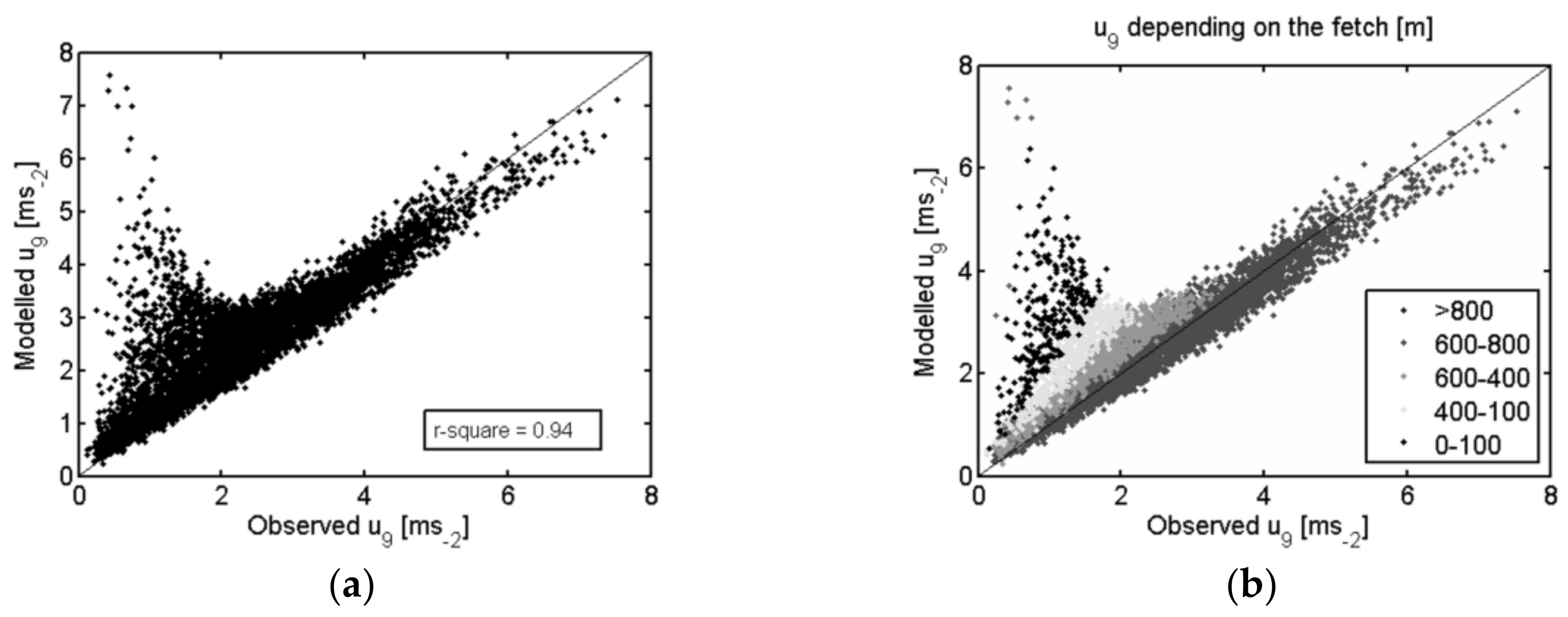
Aerodynamic Resistance Scheme and Wind-Speed Profile

The aerodynamic resistance formulations for R_A, R_S, and R_X used to derive soil and canopy H, were calculated following Norman et al. [16] and Kustas and Norman [17]:

$$R_A=\left(\left[\ln \left(z_u-d_0/z_{0\mathrm{M}}-{\Psi }_M\right)\right]\left[\ln \left(z_T-d_0/z_{0\mathrm{M}}-{\Psi }_H\right)\right]\right)/\left(k_{\mathrm{vk}}^{2}u\right),$$

(13)

where $z_u$ and $z_T$ (m) are the measurement heights for wind-speed and air temperature, respectively, d₀ is the zero-displacement plane (m), $z_{0M}$ is the roughness length for momentum transfer (m), k_vk is the Von Karman constant and Ψ_M and Ψ_H are the atmospheric stability functions for momentum and heat, derived following Dyer [38].

$$R_S=1/\left(c^{\prime }{\left(T_S-T_C\right)}^{1/3}+b^{\prime }{u}_s\right),$$

(14)

where the coefficients c′ (m s⁻¹K^−1/3) and b′ (-) were taken from Kustas and Norman [17], as used in the work of Kondo and Ishida [39]:

$$c^{\prime }=0.0025\mathrm{and}{b}^{\prime }=0.012,$$

(15)

The wind-speed just above the soil surface, $u_S$ (m s⁻¹), was parameterized following an exponential extinction law [40] as follows:

$$u_S=u_C\exp \left[-a\left(1-\left(z_S/h_C\right)\right)\right],$$

(16)

where $z_S$ (m) is the height above the soil where the effect of soil surface roughness becomes negligible, and was set equal to 0.1 for tall vegetation and 0.05 for short canopy.

Wind-speed at the top of the canopy, u_C (m s⁻¹), was then given by:

$$u_C=u\left[\left(\ln \left(\frac{h_C-d_0}{z_{0\mathrm{M}}}\right)\right)/\left(\ln \left(\frac{z_u-d_0}{z_{0\mathrm{M}}}\right)-{\Psi }_M\right)\right],$$

(17)

and the extinction coefficient a given by Goudriaan [40]:

$$a={0.28\mathrm{LAI}}^{2/3}{h}_C^{1/3}{s}^{-1/3},$$

(18)

$$R_X=\frac{C^{\prime }}{\mathrm{LAI}}{\left(\frac{s}{u_{d_0{+z}_{0\mathrm{M}}}}\right)}^{1/2},$$

(19)

C′ is assumed to be equal to 90 (s^1/2 m⁻¹), following Norman et al. [16], s was the mean leaf size (m) and u_d0+z0M was estimated following Equation (16), but using (d₀ + z_0M) (m) as the reference height;

$$u_{d_0{+z}_{0\mathrm{M}}}=u_C\exp \left[-a\left(1-\left(\left(d_0{+z}_{0\mathrm{M}}\right)/h_C\right)\right)\right],$$

(20)

2.2. Modifications to TSEB Formulations and Parameters

2.2.1. Roughness Length and Zero Plane Displacement Height (z_0M − d₀)

The aerodynamic roughness length and zero plane displacement height are two key roughness parameters in the resistance formulations and depend on vegetation characteristics. Typical values are d₀ = 2/3 h_C and z_0M = 1/3 h_C, but, in this study, both parameters were initially estimated according to [41,42] as described below:

$$u\left(z\right)/u\left(h_C\right)=\exp \left(-n\left[1-\zeta \left(z\right)/\zeta \left(h_C\right)\right]\right),$$

(21)

$$\zeta \left(z\right)={{\displaystyle \int }}_0^z\left[C_d\left(z^{\prime }\right)a^{″}\left(z^{\prime }\right)/P_m\left(z^{\prime }\right)\right]d_0{z}^{\prime },$$

(22)

$$n=\left(\zeta \left(h_C\right)\right)/\left(2u_{*}^2/u{\left(h_c\right)}^2\right),$$

(23)

$$n=\left(\zeta \left(h_C\right)\right)/\left(2u_{*}^2/u{\left(h_c\right)}^2\right),$$

(24)

$$d_0/h_C=1-{{\displaystyle \int }}_0^{1}e-2n\left[1-\zeta \left(z\right)/\zeta \left(h_C\right)\right]d_0\xi ,$$

(25)

$$z_{0\mathrm{M}}/h_C=\left(1-d_0/h_c\right)\exp \left(-k_{\mathrm{vk}}u\left(h_C\right)/u_{*}\right),$$

(26)

where u(z) is the wind-speed at height z; u(h_C) is wind-speed at the canopy; ζ (h_C) is a generalization of C_dLAI (which accounts for foliage density); C_d is the drag coefficient of the foliage elements (typically ~0.2); a″ is the vertical leaf area density, which, together with P_m, the momentum shelter factor and C_d, takes into account the vertical canopy structure [41]; $u_{*}$ is the friction velocity; and k_vk is the Von Karman constant.

Due to the vegetation characteristics of this ecosystem, Massman’s approach may not yield reliable roughness parameters, and consequently other formulations were also applied, which included [43,44]. The first approach used the second-order closure model of [45] to estimate d₀ and z_0M. The latter approach of [44], considers the tree structure and is more suitable for tall woody vegetation. This method uses observation data to fit the estimation of normalized displaced height and roughness length, related to frontal area index (FAI), which is calculated following Schaudt and Dickinson [46]. These estimates of z_0M and d₀ were compared with “observed” d₀ and z_0M derived from Las Majadas in-situ wind measurements [47,48]. To calculate d₀ and z_0M, two wind-speed measurements u₁ and u₂ (m s⁻¹) at height z₁ = 15 and z₂ = 9 (m) using cup anemometers, were combined with friction velocity, $u_{*}$ (m s⁻¹) at z_U = 15 (m) from the 3-D sonic anemometer. The 30-min average wind-speeds u₁, u₂ and $u_{*}$ sampled at 10 Hz were combined in a set of expressions based on log law for wind in the surface layer for computing d₀ and z_0M under neutral conditions following Rooney [47] and Nakai et al. [48]:

$$d_0=\frac{z_2\exp \left(k_{\mathrm{vk}}{u}_1/u_{*}\right)/\exp \left(k_{\mathrm{vk}}{u}_2/u_{*}\right)-z_1}{\left(k_{\mathrm{vk}}{u}_1/u_{*}\right)/\exp \left(k_{\mathrm{vk}}{u}_2/u_{*}\right)-1},$$

(27)

$$z_{0\mathrm{M}}=\left(z_1-d_0\right)/\left(\exp \left(k_{\mathrm{vk}}{u}_1/u_{*}\right)\right),$$

(28)

To guarantee near-neutral conditions, only data where absolute Z/L was less than 0.05 [49] with significant wind-speeds so that u₂ (z₂) > u₁ avoiding light wind cases, were used. An analysis of the model sensitivity to the aerodynamic roughness parameters was additionally performed, by incorporating the range in the magnitudes of z_0M and d₀ estimated from the approaches described above into TSEB, and evaluating the impact on the computed H and LE values. To verify the roughness-length parameters, assuming a logarithmic wind profile above the canopy, wind-speed estimations at 9 m were compared with measured wind-speed at the same height.

2.2.2. Within-Canopy Wind-Speed Profile Scheme

The within-canopy wind-speed profile, using the original exponential formulation of Goudriaan [40] and described by Equations (16), (17) and (20), may not be appropriate for forested sites [36]. Therefore, other within-canopy wind profile parameterizations proposed [21,50,51] were also tested for this ecosystem by comparing the various model computed within-canopy wind-speed at 5 m with the wind-speed measurements at 5 m above local terrain, in the tree canopy air space.

The next expression, assuming a uniform vertical distribution of the vegetation was proposed [50], following the suggestion of a wind hyperbolic-cosine profile in the lower region of the canopy [52]:

$$u_{\left(z\right)}=u_C{\left[\frac{\cos \mathrm{h}\left(\beta \frac{z}{h_C}\right)}{\cos \mathrm{h}\beta }\right]}^{\left(1/2\right)},$$

(29)

where the parameter β, similar to the extinction coefficient for Goudriaan [40], can be derived from the relationship:

$$\beta =\left(4C_d\mathrm{LAI}\right)/\left(0.16{\alpha }_{*}^2\right),$$

(30)

where C_d is the drag coefficient, typically equal to 0.2 [40], and ${\alpha }_{*}^2$ is a dimensionless coefficient that considers the presence of the roughness sub-layer of the underlying vegetative surface, taking values between 1.0 and 2.0 [53]. This parameter was set to 1, following Massman [50], based on the wind profiles of different crops.

Based on the wind-profile evaluation over a conifer forest, the wind profile within the canopy space was modeled as [51]:

$$u\left(z\right)=u_c{\left[\left(\cos \mathrm{h}\beta \left(\left(z-z_d\right)/h_C\right)\right)/\left(\cos \mathrm{h}\beta \right)\right]}^{\left(7/2\right)},z_d<z⩾h_C,$$

(31)

$$u\left(z\right){=\mathrm{C}}_c{u}_c,z_{0\mathrm{S}}<z>z_d,$$

(32)

where z_d (m) is the crown bottom height, the factor β is equal to the one from Massman [50] and the parameter C_C is defined as follows:

$$C_C={\left[\cos \mathrm{h}\beta \left(1-z_d/h_C\right)\right]}^{\left(-7/2\right)},$$

(33)

z_d was set equal to 1/3 h_C as Cammalleri et al. [21] suggested, on the hypothesis that for tall canopies the foliage occupies the upper 2/3 of the canopy height primarily.

2.2.3. Within-Canopy Wind-Speed Profile Scheme Modified to Account for Different Vegetation Layers

There are two phenological stages for grass: one is under the dry or senescent period (summer and winter), and the other is when the grass is green and actively transpiring (spring and autumn). Hence, in spring and autumn, two layers of vegetation, the trees and grass—with uniquely different phenology and physiology—are active and affecting the energy and water exchanges with the lower atmosphere. Because of the unique differences in grass and tree phenology, the wind-speed profile formulation (subscript -m) was modified by considering the effects of both oak overstory and grass understory on with-canopy wind-speed as described below:

$$u_{d_0{+z}_{0\mathrm{M}}-m}=u_{C\left(\mathrm{oak}\right)}\exp \left[-a_{\left(\mathrm{oak}\right)}\left(1-\left(d_0+z_{0\mathrm{M}}\right)/h_{C\left(\mathrm{oak}\right)}\right)\right],$$

(34)

in which the wind-speed at the top of the tree canopy, $u_{C\left(\mathrm{oak}\right)}$, is given by:

$$u_{C\left(\mathrm{oak}\right)}=u_{\left(z_u\right)}\left[\left(\ln \left(\frac{h_{C\left(\mathrm{oak}\right)}-d_0}{z_{0\mathrm{M}}}\right)\right)/\left(\ln \left(\frac{z_u-d_0}{z_{0\mathrm{M}}}\right)-{\Psi }_M\right)\right],$$

(35)

The wind-speed just above the soil surface, $u_{S-m}$ (m s⁻¹), is parameterized as in Equation (16), but using 0.05 (m) as the reference height as in:

$$u_{S-m}=u_{C\left(\mathrm{grass}\right)}\exp \left[-a_{\left(\mathrm{grass}\right)}\left(1-z_S/h_{C\left(\mathrm{grass}\right)}\right)\right],$$

(36)

with $u_{C\left(\mathrm{grass}\right)}$ being equal to:

$$u_{C\left(\mathrm{grass}\right)}=u_{C\left(\mathrm{oak}\right)}\exp \left[-a_{\left(\mathrm{oak}\right)}\left(1-\left(h_{C\left(\mathrm{oak}\right)}/h_{C\left(\mathrm{grass}\right)}\right)\right)\right],$$

(37)

factors $a_{\left(\mathrm{oak}\right)}$ and $a_{\left(\mathrm{grass}\right)}$ are taken according to Goudriaan [40] as:

$$a_{\left(\mathrm{oak}\right)}={0.28\mathrm{LAI}}_{\left(\mathrm{oak}\right)}^{2/3}{h}_{C\left(\mathrm{oak}\right)}^{1/3}{s}_{\left(\mathrm{oak}\right)}^{-1/3},$$

(38)

$$a_{\left(\mathrm{grass}\right)}={0.28\mathrm{LAI}}_{\left(\mathrm{grass}\right)}^{2/3}{h}_{C\left(\mathrm{grass}\right)}^{1/3}{s}_{\left(\mathrm{grass}\right)}^{-1/3},$$

(39)

Figure 1 displays a schema to describe the modifications in wind-speed profile following Goudriaan [40].

To be able to apply this wind modification using the total ecosystem leaf area index, which is the parameter derived from satellite remote sensing, the hypothesis of using a constant LAI for the tree canopy and a variable LAI for the understory grass layer was tested. Consequently, with an average vegetation index data of the total ecosystem, it was possible to obtain the characteristic LAI of each layer. This assumption was tested using in-situ measurement to analyze the variation of grass versus tree LAI over a growing season, as well as the oak and grass spectral information measured using in-situ radiometry (ASD FieldSpectroradiometer 3, ASD Inc., Boulder, CO, USA). After testing the hypothesis of non-variability of oak LAI (Section 3.1.2), the estimated wind-speed at 5 m was compared to measurements using the procedure described above, using the variable LAI values estimated for the grass understory and constant LAI value for the tree canopy. Total LAI was computed weighting both different LAIs by a constant fractional cover for each canopy layer (0.8 for the grass; 0.2 for the trees), determined using summertime color orthophotography for the footprint area. The oak LAI was reduced using the clumping factor computed for the trees. Values of z_0M/d₀ for the tree canopy was estimated according to [44] and were constant depending only on the oak structure. Magnitudes of z_0M/d₀ for the grass were estimated, according to Massman [41], as a function of grass LAI, which was variable during the period. Tree height (h_C(oak)) was treated as a constant over time and the understory canopy variation of the nominal canopy height (h_C(grass)) was estimated using a growth curve derived from LAI and maximum and minimum measured heights. Leaf size was also different depending on the layer (for the tree s = 0.05 m and the grass s = 0.01 m). For Massman [50] formulation, a similar approach was taken with different extinction coefficients for the tree and the grass layers.

2.2.4. Priestley–Taylor Coefficient Evaluation

The first assumption needed for computing the turbulent fluxes, the potential canopy transpiration, can have a significant influence on the final estimations [54]. Priestley–Taylor coefficient (α_PT) [37] directly conditions this initial transpiration approximation, defined as:

$${\mathsf{\alpha }}_{\mathrm{PT}}=E/E_{\mathrm{eq}},$$

(40)

where E is the evaporation rate and E_eq is the equilibrium evaporation rate. Theoretically, air passing over a saturated surface will gradually decrease in saturation deficit until an “equilibrium” evaporation rate is reached [37,55,56]. α_PT shows the relative significance of E to E_eq and thus indicates the evaporative control. In this study, the Priestley–Taylor coefficient for the whole ecosystem (grass + trees + soil) was named as α_PTS, for the canopy layer (grass + trees) α_PTC, for the trees α_PTT, and for the grass α_PTG.

Theoretical and experimental studies have shown that the value of α_PT (for the ecosystem) varies significantly with LAI, vapour pressure deficit (VPD), and soil moisture. For natural vegetation, under arid or semiarid conditions, the optimal canopy α_PT coefficient assumed lower values on average than typically observed for crops and fell even further at high values of VPD (α_PTC-[54]; α_PTS-[5]). The α_PT coefficient may also display seasonal variations [57], with minimum values occurring in midsummer, when radiation inputs are at their peak, and maximum values during the spring and autumn. Thus, adopting the standard α_PTC = 1.26 would not be appropriate for the dehesa ecosystem, since some degree of canopy stress or reduction in LE_C could be reached before the TSEB algorithm indicates α_PTC values lower than this reference due to soil evaporation becoming less than zero. In other words, the TSEB model in its current form, might not detect reduced transpiration through a reduction in α_PTC from the widely adopted initial value of 1.26 [54] due to the plant physiology.

(1) Using the values measured in the eddy covariance tower, the α_PTS coefficient (soil and canopy) and its behavior over this ecosystem (E/E_eq) were tested, computing E_eq as:

$$E_{\mathrm{eq}}=\left(\mathsf{\Delta }/\left(\mathsf{\Delta }+\mathsf{\gamma }\right)\right)\left(R_n-G\right),$$

(41)

and using measured values by the eddy covariance tower (ECT) as input data. The relationship with VPD was also analyzed. In forest environments, this approach has been adopted to compute the α_PTC [58], but, in this case, with the low tree fractional cover, it was not possible to isolate the influence of the soil and the Priestley–Taylor coefficient was a bulk one. (2) Based on ground data, an attempt was made to evaluate the α_PTT, taking only the trees into account, by assuming that during the summer the understory grass was dry and all the latent heat flux measured by the ECT system should come from tree transpiration. For the calculation of the α_PTT Equation (40) was inverted with Rn_C computed assuming an exponential extinction to the measured net radiation (Beer’s Law). (3) A statistical process was also performed to assess the α_PTT value under the conditions of the study, applying the TSEB model to the ecosystem when only trees were actively transpiring and the understory was dry (during the summer), assuming a constant LAI for oaks (using ground-truth measurement over the area) using both: (a) a green fraction equal to 1; and (b) green fraction values derived from MODIS (f_g < 1). It was analyzed using an optimization scheme similar to that of Agam et al. [54], iteratively running the TSEB with the radiometric temperature derived from the four-way radiometer (i.e., the up-welling longwave measurements), over a range of initial α_PTT values ranging between 0.5 and 1.5, with increments of 0.05. After each run, modeled LE was compared to the measured flux, analyzing the results with the Root Mean Square Difference statistic. Monthly averages of half-hourly RMSD for each α_PTT value were computed and evaluated. The best fit was taken as the optimal α_PTT for the canopy.

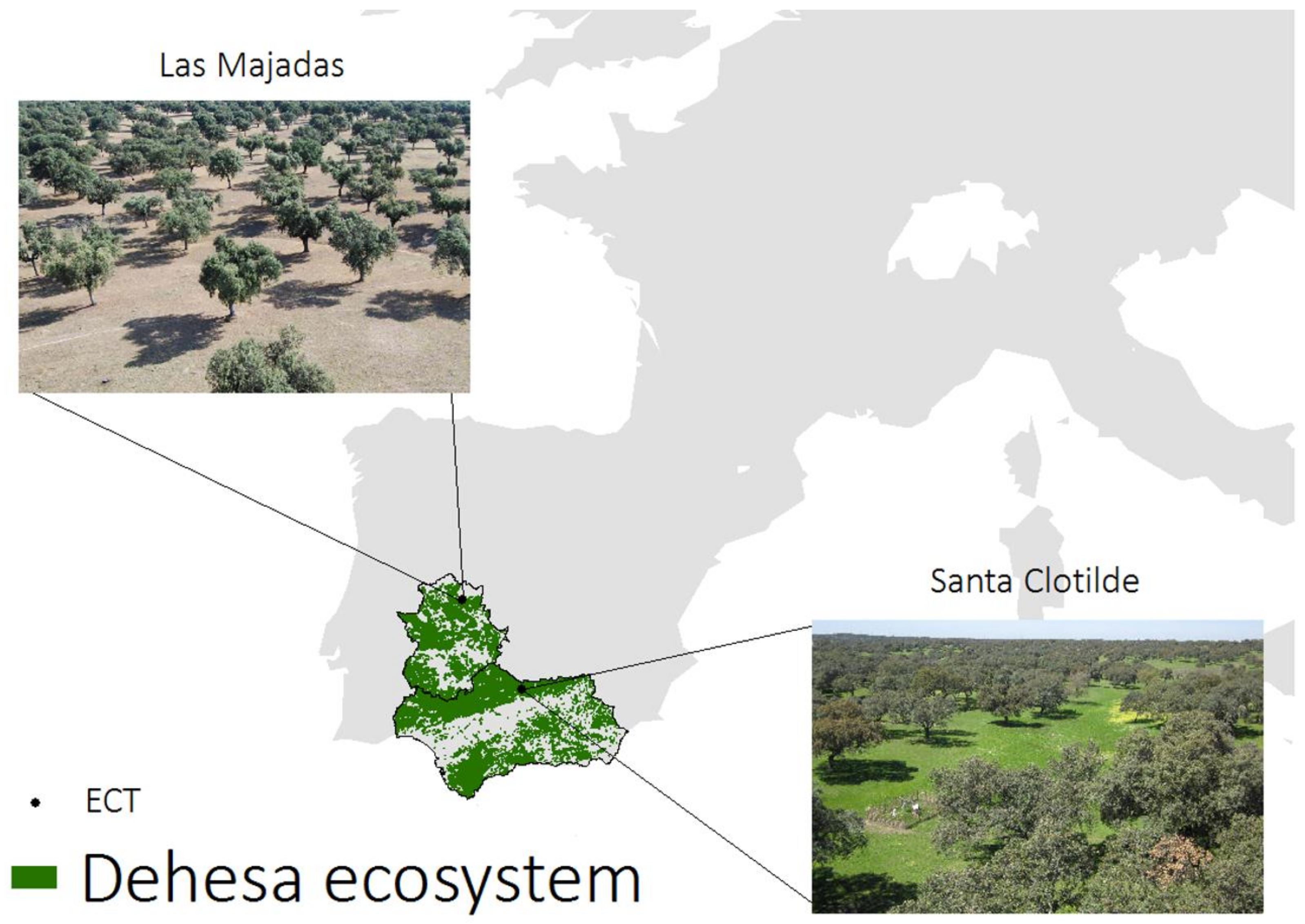
2.3. Ground Measurements (TSEB Inputs and Validation)

Data from two different dehesa sites (Figure 2) equipped with energy flux measurement systems and meteorological stations were used to evaluate TSEB formulation and as an input (wind-speed, air temperature and humidity, and solar radiation). One tower was installed in Southern Spain (Santa Clotilde, Andalusia, 38°12′ N; 4°17′ W, 736 m a.s.l.) with a 1 km homogeneous fetch along the principal wind direction (SW) and the other in Southwestern Spain (Boyal de Majadas del Tiétar, Extremadura, ES-LMa, 39°56′ N; 5°46′ W, 260 m a.s.l.) within the Fluxnet network, with a 1.5 km fetch on the NE wind direction and 2 km on the SW. Data from 2011 of the Las Majadas experimental site were used to study the behavior of the wind-speed profile, z_0M and d₀. Both experimental sites were used to estimate the energy stored within the biomass using a simple approach based on meteorological data. Due to the possibility to derive thermal information from the four-way radiometer located over Las Majadas, this site’s data (2007–2011) were used to perform the statistical analysis of the Priestley–Taylor coefficient and to derive Priestley–Taylor bulk coefficient. Measurements taken over Las Majadas during 2008 and 2009 were used to evaluate the different versions of TSEB. In-situ data collected over Santa Clotilde, from 2012 through 2014, were used to study the evolution and structure of the canopy and the annual cycle of vegetation phenology (leaf area index, fractional cover, and green fraction).

2.3.1. Santa Clotilde

This site is part of the Natural Park Sierra de Cardeña y Montoro. It is a homogeneous landscape with smooth topography, medium slopes (<10%) and a predominance of oaks (mostly Quercus Ilex. L. with an estimated mean age of 170 years, σ = 40), with sparse shrub vegetation (Cistus ladanifer L. and C. albidus L.) [59], and extensive livestock (pigs and cattle). The continental Mediterranean climate in this area is characterized by an average annual temperature of 15.3 °C and annual average rainfall of 720 mm, with cold winters, long dry summers and severe periodic droughts, the principal climatic characteristic being the annual variability and irregularity of rainfall. Soils are regosols mainly composed of sand with acid granitic bedrock [60], with a maximum depth of 1.5 m, and 0.6 m on average. Bulk density (BD) was measured with a metallic cylinder of known height and diameter, being equal to 1.57 g cm⁻³. Significant parameters for the description of canopy structure were determined in-situ, such as oak leaf size (s = 0.02 m), canopy height (h_C, with constant average tree height of 8.5 m, and a seasonal variation for the grass layer, with a maximum height of 0.7 m in April/May and dry in the summer and winter periods), average height of the first branch (FBH = 2 m), average diameter of the trees measured at breast height located at 1.3 m (DBH = 0.48 m) and crown width estimated with high spatial resolution images (CW = 7 m).

All energy balance components, Rn, G, H and LE, were measured in-situ; Rn, H and LE at 17 m height, during the study period (15 April 2012 to 31 July 2014) with an eddy covariance tower (ECT). For turbulent components of surface energy balance, the wind-speed was measured with a CSAT 3D sonic anemometer (Campbell Scientific, Logan, UT, USA), and specific humidity with a fast response hygrometer (KH20, Campbell Scientific). The anemometer was oriented in the prevailing wind direction (southwest). The separation between the sensors was 20 cm, in accordance with the manufacturer’s recommendations and the height of the tower. These measurements were recorded in a datalogger (CR1000, Campbell Scientific) at 10 Hz. For processing the data at high frequency, temperature and humidity were measured independently using a probe (HMP155, Vaisala, Helsinki, Finland). A net radiometer (NR-Lite, Kipp & Zonen, Delft, The Netherlands) located in the tower measured net solar radiation, with no interference from the other instruments, and was corrected for wind-speed in accordance with the manufacturer’s recommendations (Campbell Scientific). The post-processing of the turbulent flux data was done using TK3 application [61], which includes the necessary corrections, and footprint analysis if required. After processing, half-hourly average values of the turbulent energy balance components were obtained.

Soil heat flux was determined by ground heat flux plates (model HFP01, Huseflux, Delft, The Netherlands) installed in two grazing exclusion areas to take the heterogeneity of the area into account, one site was located over open grass and the other under an oak, at a depth of 0.08 m, with two thermocouples buried at 0.02 and 0.06 m [62]. The regular presence of livestock prevented the selection of a more distributed installation of the soil sensors over the area. Grazing conditions were reproduced in the exclusion areas. Half-hour averages of measurements, taken every 5 s were recorded by a CR1000 datalogger. Heat flux on the ground was calculated by adding to the direct measurement of the soil heat fluxes at a particular depth, the energy stored in the layer above the flux plates (Sg). The soil water content was measured during the first study period (2012) as the difference between the wet and dry weights of five random samples, taken at intervals of 10–15 days of frequency extracted every 30 cm until the maximum depth. For the rest of the period, five humidity soil probes (EnviroSCAN, Sentek Technologies, Stepney, Australia) measuring continuously at depths of 10, 30, and 50 cm, were installed inside the grazing exclusion areas.

Local leaf area index (LAI) measurements were made in-situ during 2013 to 2014 using a linear Ceptometer AccuPAR (model LP-80, Decagon Devices, Pullman, WA, USA) following the distribution of the ecosystem, integrating the relatively constant oak LAI along with the herbaceous layer LAI, with high seasonal variation. Only measurements on clear days, without cloud coverage and at nadir solar position (at approximately 12 h GTM) were taken. Local oak LAI data from another campaign were also evaluated [63]. Measurements of oak and grass spectral responses were taken in-situ during each growth state using a portable system to study the seasonal variability of the vegetation. Reflectivity measurements were taken using the ASD FieldSpec 3 spectroradiometer (ASDInc.), which registers radiance data in the range 350–2500 nm; a reference panel calibrated in a laboratory was used (Spectralon, Labsphere, North Sutton, NH, USA) to measure incident radiation for calibration purposes. Spectral measurements were taken on days without clouds and under stable weather conditions, 11:00–13:00 GMT, to minimize the effects of shadowing and solar zenith changes. Around 20 samples with a bare fibre (FOV = 25°) were taken over different mature and young trees, at 0.5 m height from the leaves. The understory was more variable, with different species, canopy heights, fractional cover and green fractions. Fifty measurements were taken at 1 m height above the soil, with a visible area diameter equal to 0.93 m. The sampling strategy for leaf spectrum gathering is described in [63].

2.3.2. Las Majadas del Tiétar

The second study site is a typical dehesa composed of an herbaceous stratum of native pasture and a tree layer of scattered oak trees, with 98% of the trees being Quercus ilex. The tree density is about 20–25 trees/ha with a mean DBH of 45 cm (measured in October 2006) and a mean tree height about 8 m. The Quercus ilex spp. are accompanied by an herbaceous understory with very high species diversity, and gentle slopes (<5%). Ten percent of the trees are pruned every winter (in January). The ground fractional cover value of the oaks (f_C), derived with the same method as for Santa Clotilde, was found to be about 20%, identical to the value estimated previously by the site team at ECT footprint scale.

The site is overall flat, with local gentle slopes of <5%. The soil is classified as Dystric Cambisol (FAO, 1985). The upper layer (~0.4 m depth) soil texture is sandy loam, with a bulk density of 1.59 g cm⁻³. Soil depth is important, and it is much larger than 3 m. The climate is Mediterranean with continental influence, with a mean annual temperature of 16.7 °C and mean annual precipitation of ca. 650 mm with large inter-annual variability. The site is used for continuous grazing of extensive livestock with a low density of 0.3 cows/ha. During the driest summer months (July–September), most of the cattle is moved to nearby mountain grasslands.

The eddy covariance flux measurements were performed at 15.5 m height using an open-path IRGA (LI-7500, LICOR Inc., Lincoln, NE, USA) and a 3-D sonic anemometer (R3-50 Solent, Gill, Lymington, UK). The EC raw data were processed using Alteddy v3.72 software (Alterra, Wageningen) to calculate fluxes at 30-min time scale, following the CarboEurope IP methodology for both flux processing and flux quality checking [64]. Solar and infrared radiation components were measured using a fouf-component net radiometer (CNR1, Kipp & Zonen), used to derive radiometric surface temperature, and soil heat flux was estimated using four soil heat flux plates (HFP-01EC, Hukseflux). The air temperature and relative humidity were measured at 8 m height with an Hygro-Thermo transmitter (Thies Clima, Goettingen, Germany) and the atmospheric pressure with a barometric pressure sensor (Model 276 Setra, Boxborough, MA, USA). Horizontal wind-speed and wind direction were measured at heights of 15, 9, and 5 m with 2-D sonic anemometers (Windsonic, Gill), as were separate surface temperature from the tree and the grass/soil during 2011.

LAI in-situ measurements used here were performed between 2006 and 2011. Only one single LAI value was derived for trees, because this parameter was assumed to present low seasonal and inter-annual variability, while understory LAI estimates were performed with varying frequency (from monthly to three-monthly). The LAI of the grass exhibited a significant seasonal variation, with minimum values over the summer dry season (June–October, LAI << 0.1) and seasonal peak values in spring (0.9–2). Understory LAI was estimated by destructive sampling (12 samples of 25 × 25 cm, 4 of them below the tree canopy). All samples were then separated into their dry and green fractions (excluding moss lichen panicles and flowers) before scanning subsamples of green fractions for estimating ecosystem scale LAI. Tree LAI value was calculated as the average of tree LAI estimates performed according to two independent methods. The first one was based on single tree LAI estimates (measurement performed on nine trees with LAI2000 using four rings for calculation) and extrapolating this value to the whole ecosystem, assuming a canopy cover fraction of 20%. The second method was based on site-specific measurements (SLA = 45.95 cm² g⁻¹) and an estimate of foliage biomass from allometric relationships (based on DBH distribution from a survey of 244 trees in a 12.46 ha area surrounding the tower).

2.3.3. Energy Balance Closure Error and Footprint

The energy balance closure (EBC) error [65,66] was used to describe the quality of the data-flux series collected. To determine the area that contributed most to the measured fluxes at the tower, and assure sufficient fetch for remote sensing integration, an approximate solution for the contribution to the vertical flux [67] was computed. A meteorological station was installed inside the open grass exclusion area, which measured variables of interest such as direct solar radiation and precipitation. For ecosystems with tall vegetation, [66] recommended the energy storage within the biomass (S) to be determined as part of the total energy balance (e.g., Rn = G + H + LE + S). Therefore, the magnitude of S for this ecosystem was estimated using a simple approach [68,69], based on meteorological data, due to the lack of necessary measurements of biomass heat storage in-situ. However, these estimates of S are considered a reasonable proxy [70].

2.3.4. Remotely Sensed Inputs for TSEB

Local LAI from grass and oak were inferred from in-situ reflectance measurements to determine whether the derivation of LAI using the broad bands from satellites could be used as a proxy, and supported the assumption of non-variability of the oak canopy spectral properties throughout the year when extrapolating the estimates. We used the scaled NDVI approach method described by Choudhury et al. [71] to retrieve LAI from remote sensing data.

The fraction of vegetation that is green and transpiring (f_g, Equation (11)), involved in the computation of the canopy transpiration, was adjusted using remote sensing data, following the suggestions of Guzinski et al. [22], to reflect the current phenological conditions. Values of f_g were estimated using vegetation indices (VI), as computed by Fisher et al. [72], with the NDVI and the enhanced vegetation index (EVI) obtained from MODIS sensor data. To compare in-situ derived f_g values with those from the satellite, ground reflectance measurements of each vegetation layer, taken with an ASD FieldSpectroradiometer (FieldSpec 3, ASDInc.), were processed to simulate MODIS bands to compute the VIs. Each estimation of f_g was weighted by the area occupied by each component within the ecosystem. This was only possible on three days on which spectral measurements were made over both oak and grass, in July 2013, May 2014 and June 2014. These VI values were then compared with the VI derived with MODIS, with daily coverage and 250 m of spatial resolution for the visible and near infrared bands (MOD09GQ and MOD13Q1 products).

The bulk ecosystem surface temperature was estimated from the upwelling (LW_OUT) and downwelling (LW_DN) longwave radiation using the following equation:

$${\mathit{LW}}_{\mathrm{OUT}}=\left(1-\mathsf{\epsilon }\right){\mathit{LW}}_{\mathrm{DN}}{+\mathsf{\epsilon }\mathsf{\sigma }T}_{\mathrm{RAD}}^4$$

(42)

where σ is the Stefan–Boltzmann constant and ε is the surface emissivity, computed using woody savannas vegetation emissivity and soil emissivity, weighted by f_C [73].

2.4. Evaluation of TSEB Performance in the Dehesa

Different estimates of roughness parameters, within-canopy wind profile formulations and values of the Priestley–Taylor coefficients for TSEB were tested, as detailed in

Table 1. Defining the acronyms for the different TSEB computations based on estimates of d₀ and z_0M using Massman [41] for grass or combined grass-oak system, or Raupach [44] for oak or combined grass-oak system, wind-speed profile in the canopy layer using Goudriaan [40] or Massman [50] and α_PTC = 1.26 or 0.9.

	TSEB-GM	TSEB-GR	TSEB-MR	TSEB-GGT	TSEB-MGT	TSEB-GM-PT
d0 − z0M
Massman [41]	x			x (grass)	x (grass)	x
Raupach [44]		x	x	x (oak)	x (oak)
Wind-speed profile
Goudriaan [40]
a	x	x				x
a(oak)—a (grass)				x
Massman [50]
β			x
β(oak)—β (grass)					x
αPTC
1.26						x
0.9	x	x	x	x	x

. The various modifications to TSEB were applied with radiometric surface temperature derived from in-situ upwelling longwave radiation. Table 1 presents the formulations for d₀ − z_0M and the wind-speed profile used in each version of the model and the denomination given to each one, for a better understanding of the procedure:

3. Results

3.1. Evaluation of the Ground Measurements and TSEB Inputs

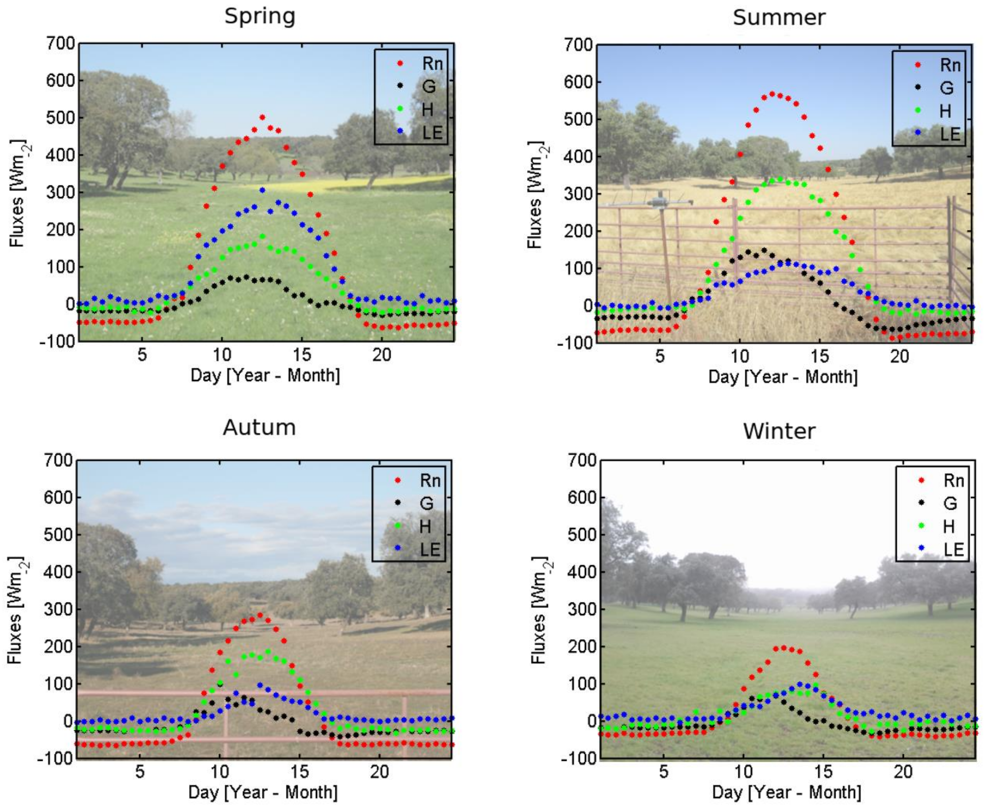
3.1.1. Evaluation of the Surface Energy Fluxes Measured at the EC Sites

Direct measurements of the four energy balance components were evaluated in both study areas, yielding average closures of 80% for Santa Clotilde and 86% for Las Majadas, both within the error range found by other authors [66,74]. These quantities represented absolute errors of 49 W m⁻² and 40 W m⁻², respectively. Better ECB was observed during the summer and winter times. In Santa Clotilde, this can be due to less noise derived from rainfall events and condensation processes occurred during these periods. Lower values of LE were seen to be directly correlated with better closure balance, which, with this flux being very low during dry periods, could indicate higher uncertainty in LE measurement than in H. This is consistent with the Las Majadas analysis done by Perez et al. [75]. LE has two peaks, in the spring and autumn, related to the typical rainfall temporal distribution. However, the magnitude and timing of precipitations can vary significantly from year to year.

The typical seasonal pattern of flux variation corresponded to that of semiarid Mediterranean areas, with wet-cold and hot-dry periods (Figure 3). In dry periods, H reached maximum value in the middle of the afternoon, while the soil heat flux did so earlier, to reach the minimum after dark. The latent heat increased during the day, but remained low due to the lack of available water in the soil for transpiration or evaporation. In contrast, during wet seasons, LE was higher than H, while G values declined, probably due to the effect of the grass layer, covering the soil and intercepting most incoming radiation. Due to the often lesser importance of the soil heat flux compared to the other components, many studies have simplified the estimated energy balance by discarding this flux on daily scales. However, in savanna type ecosystems, G may represent more than the 20% of the net radiation during summer, similar to or even higher than the latent heat flux, with sensible heat flux reaching values higher than the 45% of Rn. These observations are consistent with the dry summer climatic conditions of the area, during which the water shortage influences strongly the partitioning of available energy between the observed sensible and latent heat fluxes [76]. During the wet season, the opposite trend is observed.

The analysis of the energy storage within the biomass, according to Stewart and Thom [68] and Stewart [69], revealed that the relative importance of this component on the overall balance was very low, with monthly average values ranging between zero and less than 10 W m⁻², which is 3% of the available energy. Unfortunately, ground measurement of this component is difficult, and the small magnitude of the estimated values suggests that it is likely to be a relatively small term for this ecosystem. However, the storage term can be larger for other areas in the dehesa with higher tree ground coverage. For example, Kobayashi et al. [77] evaluated S for an oak savanna with fraction tree cover of 50% and the storage term accounted for on average 12% of the available energy over the daytime.

The area that most contributed to the energy fluxes measured by the Santa Clotilde ECT was located between 0 and 500 m in the predominant wind direction, where 60% of the fluxes captured were generated, reaching 80% within 1000 m, with the maximum in the first 200 m. At Las Majadas, the peak contribution is located within 500 m, with 70% of the flux captured by the ECT coming from the area between 0 and 500 m, reaching almost 90% in the first 1000 m. Given these results, and considering that the same land use is extended and uniform at least 1000 m along the principal wind directions (SW for Santa Clotilde, SW and NE for Las Majadas), no problems of fetch might be expected, taking ECT data measured over the principal wind component. In the same way, it is possible to integrate information from medium-resolution (pixel size between 30 and 120 m) and even low-resolution (250 m⁻¹ km pixel size) Earth observation satellites.

Both areas are located around 200 km away, but they share the same ecosystem, management practices, meteorological conditions and vegetation ground fractional cover. All these similarities led us to reasonably consider extrapolating the results from one area to the other, and probably to almost the whole dehesa in this region, due to the constant qualities of this ecosystem. However, at this large scale, the influence of differences in f_C and meteorological conditions need to be taken into account.

3.1.2. Evaluation of the Remote Sensing Data Used to Derive TSEB Inputs

Analysis of the variations in oak and understory leaf area index measurements over the course of the year (2013–2014 Santa Clotilde and 2006–2011 Las Majadas) indicated that the oak LAI exhibited a fairly constant value compared to the understory LAI. In Santa Clotilde, the mean local oak LAI was 2.60, with a standard deviation of 0.13. The annual LAI mean for grass was 0.62 (σ = 0.69) in Santa Clotilde and 0.42 (σ = 0.48) for Las Majadas. Both deviations showed the variation of the herbaceous index compared with the tree index.

For Santa Clotilde, local LAI of grass and oaks were derived from in-situ spectral information to determine whether the derivation of LAI using the broad bands from satellites could be used as a proxy, and supported the assumption of non-variability of the oaks’ spectral properties throughout the year when extrapolating the estimates. The oak spectral information collected reveals that, even when the variation is perceptible over the seasons, the ratio between the regions used to derive LAI as a function of NDVI remained constant. The grass spectrum over the season has greater variations due to the growing cycle of this annual vegetation, which in the year ranges between almost full cover to bare soil/dry grass. The error when compared to local oak and grass LAI derived from the ground-based spectrometer and the measured index was 27% and 28% respectively. When conducting a simple model sensitivity analysis to LAI on these conditions, a variation on the value of 30% would increase the final model error on a range of 4% to 7%. Averaging the measured spectrum using MODIS spectral filter bands, the estimated local LAI value for oaks was 2.294 (σ = 0.092) and for grass, 0.64 (σ = 0.82), similar to the ground measurements averages. Considering the uncertainties around the ground-based spectral measurements of LAI, and on the formulations used to derive this parameter, converting remotely sensed information of vegetation indices to LAI values for oaks/grasses in this ecosystem is sufficiently accurate. When comparing ground measurements with land surface variables retrieved from earth observation data, the mismatch between the data footprints (representativeness), and the uncertainty introduced by the variables scaling and the formulations used, have to be evaluated in order to characterize the error accurately. The results from ground LAI measurements and ground-based spectrum measurements observations suggest that the assumption of a constant oak LAI during the year is acceptable for the purposes of this study.

To account for the clumped vegetation structure of dehesas, the clumping factor was estimated following Kustas and Norman [12]. In Las Majadas the clumping factor Ω(0) found for the trees was 0.71, and 0.61 for Santa Clotilde. For the estimation of the clumping factor at solar zenith angle φ, distance between trees was evaluated using GIS techniques, averaging the distance between consecutive trees over both areas, giving a rough mean value of 30 m.

Comparing f_g values for Santa Clotilde derived from MODIS and spectral data (

Table 2. f_g estimated from in-situ spectra using MODIS bands functions and f_g estimated from MODIS products for Santa Clotilde.

Date	fg from Spectral Information			fg from MODIS
	Oak	Grass	Oak + grass	Oak + grass
23 July 2013	0.73	0.75	0.75	0.81
23 July 2013	0.76		0.75	0.81
20 October 2013		0.78		0.66
20 December 2013	1
7 April 2014		0.94
5 May 2014		0.98	0.98	0.74
13 May 2014		0.87	0.9	0.74
19 May 2014	1
30 June 2014	0.78	0.82	0.81	0.71

), no definitive conclusions about the goodness of the adjustment of MODIS index could be drawn, due to the low number of samples and the possible mismatch between data footprint. Although it seems that the MODIS-derived indices are higher than the spectral-derived indices in summer and the opposite situation is found during spring. Even when the grass is completely dry, f_g values derived from MODIS are still high (e.g., August 2013 = 0.81). f_g derived from the satellite incorporates the effect of the evergreen vegetation along with the grass, but considering the low tree fractional cover in these ecosystems, a strong influence would not be expected. It may be that this parameter does not reflect phenological conditions during the dry period sufficiently accurately for these ecosystems, with considerable seasonal variations.

3.2. Evaluation of TSEB Formulation

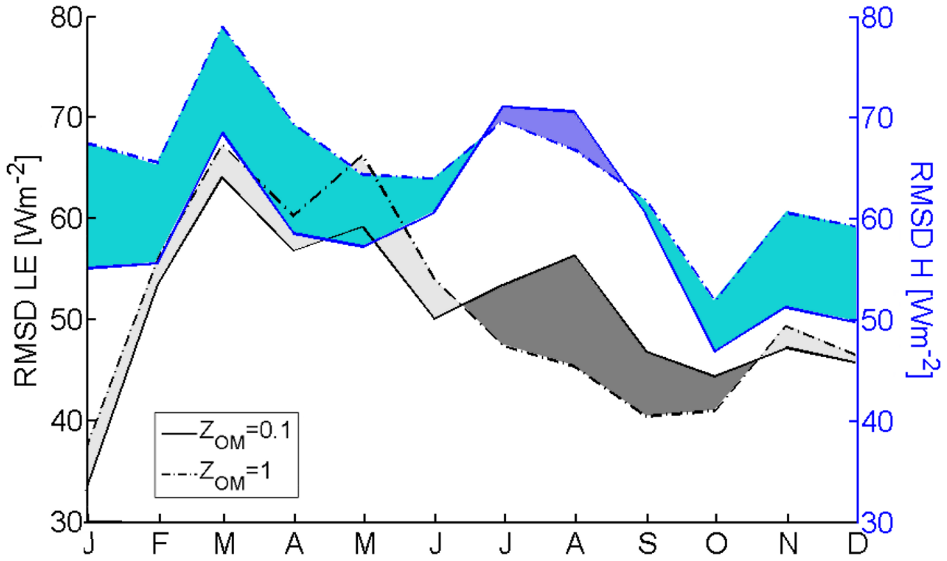
3.2.1. Roughness Length and Zero-Plane Displacement Height

The comparison between estimated versus measured d₀ indicate that it was less influenced by the formulation selected than the roughness length, with an uncertainty of 25% for all the approaches. A sensitivity analysis of d₀ influence on TSEB was performed with d₀ values ranging from a minimum of 1.5 to maximum of 4 m. The results showed that the maximum variation in flux estimation caused by the value adopted for d₀ was less than 1 W m⁻² for LE and 4 W m⁻² for H.

The best adjustment for the roughness length was given by the Raupach [44] formulation (45% MAE), which integrates the vertical structure of the trees, but not for the grass. Meanwhile, Choudhury and Monteith [43] produced a MAE equal to 125% and Massman [41] equal to 140%. All formulations tend to overestimate the observed z_0M value (

Table 3. Different average values (m) of d₀ and z_0M using the different approaches (“observed” values are computed using Rooney [47] and Nakai et al. [48] as described in the previous section) for Las Majadas.

	“Observed Values”	(2/3 hC) and (1/8 hC)	Raupach (1994)	Choudhury and Montheith (1988)	Massman (1997)
d0	Mean: 3.35 Std: 1.94	5.33	5	Mean: 4.66 Std: 0.23	Mean: 4.05 Std: 0.43
z0M	Mean: 0.52 Std: 0.3	1	0.687	Mean: 1.13 Std: 0.2967	Mean: 1.24 Std: 0.06

), which is smaller (x = 0.52 and σ = 0.3) than the one expected for this tall vegetation environment (~1), possibly due to the low fractional cover of the oaks.

The z_0M range (0.1 to 1 m) was used in the TSEB sensitivity analysis, as presented in Figure 4, resulting in a variation of 20 W m⁻² (20%) in the sensible heat flux, an order of magnitude larger when compared with d₀. Variations in the value of z_0M affect the computation of the resistances and wind-speed profile, and, as a result, the overall fluxes. A lower z_0M would lead to a higher R_A (Equation (13)), and also lower R_X (Equation (19)), due to the increase in canopy wind-speed. This higher u_C will result in a higher wind-speed at soil level, resulting in lower R_S (Equation (14)). Consequently, a larger H_S is expected while a higher R_A but lower R_X generally reduced h_C because the value of R_X is less influenced by the value of z_0M and u_C than R_A or R_S, with mean differences between the resistance values for z_0M = 0.1 and z_0M = 1 corresponding with 50 s m⁻¹ for R_A, 20 s m⁻¹ for R_S and less than 1 s m⁻¹ for R_X.

Figure 4 shows the variation in sensible heat flux RMSD for a given number of roughness length values during the year. During the summer, the model appeared to be less sensitive to roughness length variations, probably because the differences between the canopy/soil and air temperatures were markedly more significant during this season. It can also be observed that when z_0M reached a threshold value, H RMSD reached a limit and higher z_0M values do not increase the errors. For LE, during the summer (Figure 4), higher z_0M values would reduce the error. Higher z_0M facilitates the sensible heat flux transport, with a decrease in R_A at the expense of latent heat flux, improving the simulation of low LE rates over the dry season.

The formulation, developed to modify the wind-speed profile scheme to account for different vegetation (grass and tree) layers (Section 3.2.2), includes Raupach formulation [44] for computing oak d₀ and z_0M (function of tree vertical and horizontal structure) and Massman formulation [41], which yielded good results in previous studies with herbaceous vegetation [16,17,21] for the grass understory d₀ and z_0M, as a function of the LAI and the height.

The MAE in the estimate of wind-speed at 9 m integrating d₀ and z_0M with Raupach [44] (outside the canopy layer) using a simple logarithmic approach considering stability effects was 20%, with r² of 0.94 (Figure 5a). The errors were highly dependent on the fetch influencing the measurements, with significantly higher errors when the fetch was up to the first 100 m (Figure 5b). This low fetch reflects low wind-speeds and highly unstable conditions that can increase the error in the stability corrections algorithms significantly. Under these highly convective conditions, the stability-corrected logarithmic profile may not apply to the current stability formulations [38,78].

3.2.2. Within-Canopy Wind-Speed Profile Scheme

With regard to the estimates of wind-speed at the height of 5 m (within the tree canopy layer), the three formulations tested [40,50,51] yielded errors of 32%, 43% and 99%, respectively (Figure 6). The Lalic model estimates a strong within-canopy extinction of the wind-speed, yielding a very low wind-speed at 5 m, agreeing with the results found by Cammalleri et al. [21]. Given these results, the Lalic model was discarded for the later applications of the TSEB model. Differences in the wind-speed slope may correspond to different seasons and consequently different leaf area indices, with the existence of the herbaceous canopy layer at different phenological stages (dry/senescent versus green and actively growing) influencing the relationship.

3.2.3. Within-Canopy Wind-Speed Profile Scheme with the Modification to Account for Different Vegetation (Grass and Tree) Layers

When the modified wind-speed profile was applied to the data (Equations (34)–(39)), the error in the estimation of wind velocity at 5 m was reduced to 24% using the Massman approach and 28% using Goudriaan (Figure 7). This formulation takes into account that the wind-speed from a height of 9 m to 5 m will be attenuated by the tall vegetation, and the extinction coefficient should be determined by tree layer.

These results indicate that the Massman formulations for estimating with-in canopy wind-speed may give slightly more reliable estimates than Goudriaan. as found by Cammalleri et al. [21] for an olive orchard, while no measurements under the grass canopy layer were available, preventing a complete test of the assumption that separate extinction coefficients for each canopy layer might be a suitable solution for this ecosystem. Nevertheless, the use of an “oak extinction coefficient” for the wind-speed estimate at the height of 5 m, instead of an extinction coefficient which integrates the whole ecosystem LAI, seems an appropriate solution under the conditions studied.

3.2.4. Priestley–Taylor Coefficient Evaluation

Initially, a constant measured LAI for oak trees, with a constant clumping factor of 0.71 and f_g = 1 was assumed. This was followed by incorporating a variable f_g determined from remote sensing, to analyse the influence of the different vegetation conditions. The selection of a P-T coefficient value for oak trees focused on data collected during the summer and winter. However, it is interesting to examine the results of the interaction over the course of a year (Figure 8). Even over extended periods, mainly during the autumn and spring, values corresponded to the co-existence of two contrasting vegetation layers, which are contributing to ET, in this case oak trees and grasses. Comparison between LE observed and estimated for the dry period with Priestley–Taylor coefficient equal to 0.5 is RMSD = 55 W m⁻², 0.9 RMSD = 60 W m⁻², and 1.26 RMSD = 71 W m⁻².

This analysis showed that the Priestley–Taylor coefficient displayed seasonal variations under these conditions, confirming previous findings [57], with minimum values occurring in mid-summer, when radiation inputs were at their peak, and maxima occurred during the spring and autumn. During winter, spring and autumn, the error found for LE with both applications was similar for every Priestley–Taylor coefficient selected. The higher error in March may be due to rainfall events and condensation processes affecting both modeled and measured fluxes. During the summer months, the smallest RMSD values for LE was found with α_PT = 0.5 either using f_g = 1 or variable f_g. However, there is little increase in the magnitude of RMSD for α_PT between 0.5 and 0.9, and it is only when the standard value α_PT = 1.26 is used, does the RMSD increase by ~10 W m⁻² to nearly 65 W m⁻². This translates to approximately a 20% error in LE using either f_g = 1 or a variable f_g. Although the lowest RMSD for LE over the summer months corresponded to α_PT = 0.5, even taking into account the green fraction, using α_PT = 0.5 had the highest error from January through May. This can be caused by the combined effect of f_g and α_PT = 0.5 in reducing transpiration.

The maximum value of an oak woodland α_PTS for a similar ecosystem was found to be about 0.9, 30% less than values associated with evaporation from green, well-irrigated and fertilized crops such as wheat [5]. In the forest, observational studies found that unstressed α_PTE y was significantly lower than the typical value of 1.26. Some of these values found for temperate broad-leaved evergreen forest were: 0.99 [79], 0.65 [80], 0.93 [81], 0.61 [82], 0.64 [83] and 0.72 [84,85,86]. For a temperate broad-leaved forest a mean value of 0.82 ± 0.16 was found [58]. All these studies suggest that natural vegetation displays a value of α_PTT that is lower than the standard for crops, reflecting the relatively conservative water-use tendencies of semiarid natural vegetation adapted to these environments. Considering previous studies and the results presented in this section, Priestley–Taylor coefficient value was modified to 0.9 for the whole ecosystem. In doing so, the RMSD values were reduced by ~10 W m⁻² for the summer period.

P-T bulk coefficient: Priestley–Taylor coefficient for the total ecosystem

α_PTS bulk monthly averages estimations (Figure 9 on bulk Priestley–Taylor) during the day, ranged from a maximum value of 0.85 in May to a minimum value of 0.2 in August. In this area, equilibrium LE is higher than or equal to LE, so that the coefficient will vary between 0 and 1. Mean standard deviation over the whole year was 0.32, with maximum values occurring in winter (~0.4) and minimum values occurring in the summer (~0.2). This is likely due to the existence of different sources of ET during winter months, with trees (mostly dormant), but some grasses are transpiring because water is available and due to soil evaporation during and after rains, which is when most of the precipitation occurs. In contrast, in the summer, there are extended dry periods with very little, if any, precipitation, with only oak trees actively transpiring. Monthly averages of α_PTC during daytime conditions were computed using the net radiation of the canopy (Figure 9 on Canopy Priestley–Taylor). For the summer season (from July to September) with no or little senescent grass in the understory (due to dry soils and animal grazing) and very little, if any, soil evaporation, it was assumed that α_PTC was only for the oak trees (α_PTT). The average α_PTT estimated was 0.85. Monthly average estimates of daytime α_PTC (grass + trees = α_PTT + α_PTG) outside of the summer period using Rn_C (trees + grass) was 1.2 (~1.26), which is likely to be due to the influence of the grass understory and the evaporation on the total ET. As it is shown in Figure 9, P-T bulk coefficient displayed an indirect relationship with the VPD, as suggested by Baldocchi and Xu [5] and Agam et al. [54]. This response may be related to the physiological characteristics of the natural vegetation growing in arid and semiarid environments, but a future study integrating the influence of the grasses in the calculation has to be conducted. Even though an increase in VPD enhances transpiration by producing a steeper humidity gradient between the leaf and the atmosphere, it also initiates negative feedback on stomatal conductance, which leads to a reduction in transpiration [5].

3.3. Evaluation of TSEB Performance in Savanna Ecosystem

Figure 10 compares estimated and observed fluxes for different applications of TSEB with the different roughness inputs, wind profile formulations and Priestley–Taylor α_PTC values as defined in Table 1. To improve accuracy, and to test the assumption of a constant oak LAI and variable grass LAI, the LAI measured at Las Majadas during 2008 and 2009 was used, with a clumping factor at nadir view of 0.71. As model input (air temperature and humidity, incoming solar radiation, and wind-speed) and validation data (four surface energy fluxes), the dataset collected over the same period by the eddy covariance tower was used. The Priestley–Taylor coefficient finally selected was 0.9, with f_g estimated using MODIS remote information. The roughness length formulation selected for the application of TSEB with Goudriaan [40] and Massman [50] wind profiles with the common formulation of the extinction coefficient (TSEB G and TSEB M) was that of Raupach [44]. When separate estimates of z_0M/d₀ for the trees and grasses were required, because an extinction coefficient for each canopy layer was calculated (TSEB G_GT and TSEB M_GT), Raupach formulation [44] was employed for the oak (function of vertical and horizontal tree structure) and Massman formulation [50] for the grass (function of the LAI and the height).

Table 4. RMSD for Rn, G, H and LE from the application of TSEB and the different versions with T_RAD derived from the four-way radiometer (ECT).

RMSD (W m−2)	TSEB-GM	TSEB-GR	TSEB-MR	TSEB-GGT	TSEB-MGT	TSEB-GM-PT
Rn	27	27	27.5	30	30	27
G	28	28	28	28	27	28
H	47	48	46	55	53	50
LE	50	46	46	48	44	60

lists RMSD values for every version, including the TSEB with a P-T coefficient equal to 1.26. Both Figure 10 and Table 4 show that the modified versions outperformed the direct application of TSEB in this ecosystem. TSEB G and TSEB M showed fewer disparities, but differences between the modified wind-speed profiles versions are hardly noticeable. Rn is almost invariant as well as G in all simulations. All versions (TSEB-G_M, TSEB-G_R, TSEB-G_GT, TSEB-M_R) except the Massman modified wind-speed profile (TSEB-M_GT), which calculated an extinction coefficient for each canopy layer, tended to overestimate LE for low-medium values showing the opposite trend for H. This may be because even integrating the green fraction and reducing the α_PT coefficient, during the dry periods without available water LE flux is so low as to approach zero. The original α_PT coefficient = 1.26 resulted in TSEB overestimating LE during the whole year, especially in summer.

RMSD between estimated and observed values for the energy fluxes of TSEB-G_M, TSEB-G_R, and TSEB-M_R are within the limits found by other authors for more uniform and homogeneous canopies [13,16,17,18], and is within the uncertainties of the measurement technique (~40 W m⁻²). It is worth noting that all the modified wind profile versions that accounted for the existence of different canopy layers with different extinctions coefficients yielded similar results. Both the Massman and Goudriaan models of with-in canopy wind profile yielded reasonable estimates of both fluxes, while Cammalleri et al. [21] found for a more uniformly structured/spaced tree crop (olive orchard) a slightly better performance using the Massman model.

The discrepancy between the measured and observed values of net radiation is approximately 15%, while it is 50% for the soil heat flux. The relatively large “error” in G is likely due in part to the difficulty in providing a representative sampling area for G in such a sparse heterogeneous site. The turbulent fluxes had a relative error of 35% for LE and 30% for H. During the dry period, the relative error of LE significantly increased, due to the small magnitude in measured LE. With the existence of a double canopy layer of a tree overstory and grass understory, a revision to the net radiation partitioning for both vegetation elements might further improvement to the total and the partitioning of the fluxes. Due to the magnitude of the soil heat flux in this semiarid ecosystem and its influence on the total available energy, further research is also needed to improve the measurement and modeling of G. However, the accuracy in the estimation of H and LE for a such a complex and heterogeneous ecosystem as the dehesa using the TSEB model is considered adequate for monitoring vegetation stress and encourages future applications.

4. Conclusions

The accuracy of the estimates of the energy fluxes for a natural woody cover such as dehesa by means of a TSEB model, with an adjusted Priestley–Taylor coefficient reflecting the relatively conservative water-use tendencies of this natural semiarid vegetation and a roughness length formulation which takes into account the tree structure and the low fractional covers, is considered adequate for monitoring ecosystem water use and stress. This encourages the future application of the model on a routine basis to assist in management decisions over this region integrating satellite remote sensing data to map vegetation conditions. Given the results obtained in this paper, an analysis of the distributed model application in a dehesa-type ecosystem was conducted in a second paper: “Modeling surface energy fluxes over a dehesa (oak savanna) ecosystem using a thermal based Two-Source Energy Balance model (TSEB) II—Integration of Remote Sensing medium and low spatial resolution satellite images” (in review). The TSEB model was tested with the Massman formulation for the wind-speed profile, a Priestley–Taylor coefficient of 0.9, and clumping factors over nadir of 0.71 (Las Majadas), and 0.62 (Santa Clotilde), with [44] roughness length formulation.

Based on the analysis performed, energy storage within the biomass is found to be negligible under these fractional cover conditions, although, in dehesas with more dense canopies than the studied areas, integrating this flux into the surface energy balance could improve the balance closure and further applications [77]. The results suggest that the assumption of a constant oak LAI during the year is acceptable for the purposes of this study. Similarly, the use of spectral information to derive vegetation indices for oaks and grasses in this ecosystem is sufficiently accurate to apply energy balance modeling, integrating remotely sensed data. Green fraction index, also integrated into the TSEB calculations and derived by Guzinski et al. [22], may not reflect phenological conditions during the dry period with sufficient accuracy. Although the hypothesis on a separately wind-speed extinction coefficient for each layer has not been completely addressed, the results show that for the oak this approach is more precise than taken a bulk system coefficient. Nevertheless, it is necessary to integrate the different layers not only into the wind-speed profile, but also into the radiation budget which limits the energy available for the turbulent fluxes. Considering a different Priestley–Taylor coefficient for the grass and tree layer may also be necessary, and hence integrate the total flux contribution of each vegetation layer explicitly. This integration will be the next step in the research.

References

1. Sankaran, M.; Ratnam, J. African and Asian Savannas A2—Levin, Simon A. In Encyclopedia of Biodiversity, 2nd ed.; Academic Press: Waltham, MA, USA, 2013; pp. 58–74. ISBN 978-0-12-384720-1. [Google Scholar]
2. Papanastasis, V.P. Vegetation degradation and land use changes in agrosilvopastoral systems. In Sustainability of Agrosilvopastoral Systems: Dehesas, Montados; Advances in Geoecology; Catena Verlag: Reiskirchen, Germany, 2004; Volume 37, pp. 1–12. ISBN 3-923381-50-6. [Google Scholar]
3. Schnabel, S.; Dahlgren, R.A.; Moreno, G. Soil and water dynamics. In Mediterranean Oak Woodland Working Landscapes: Dehesas of Spain and Ranchlands of California; Springer: New York, NY, USA, 2013; pp. 91–121. [Google Scholar]
4. Pachauri, R.K.; Meyer, L.A. (Eds.) IPCC Climate Change 2014: Synthesis Report. Contribution of Working Groups I, II and III to the Fifth Assessment Report of the Intergovernmental Panel on Climate Change; IPCC: Geneva, Switzerland, 2014. [Google Scholar]
5. Baldocchi, D.D.; Xu, L. What limits evaporation from Mediterranean oak woodlands—The supply of moisture in the soil, physiological control by plants or the demand by the atmosphere? Recent Dev. Hydrol. Anal. 2007, 30, 2113–2122. [Google Scholar] [CrossRef]
6. Jeltsch, F.; Weber, G.E.; Grimm, V. Ecological buffering mechanisms in savannas: A unifying theory of long-term tree-grass coexistence. Plant Ecol. 2000, 150, 161–171. [Google Scholar] [CrossRef]
7. Bond, W.J.; Keeley, J.E. Fire as a global “herbivore”: The ecology and evolution of flammable ecosystems. Trends Ecol. Evol. 2005, 20, 387–394. [Google Scholar] [CrossRef] [PubMed]
8. Andreu, A. Water Monitoring in Vegetation Covers through Multi-Scale Energy Balance Modelling Using Time Series of Remotely Sensed Data; University of Cordoba: Cordoba, Spain, 2014. [Google Scholar]
9. Campos, P. Mediterranean Oak Woodland Working Landscapes: Dehesas of Spain and Ranchlands of California; Springer: New York, NY, USA, 2013. [Google Scholar]
10. McCabe, M.F.; Wood, E.F. Scale influences on the remote estimation of evapotranspiration using multiple satellite sensors. Remote Sens. Environ. 2006, 105, 271–285. [Google Scholar] [CrossRef]
11. Gamon, J.A. Reviews and Syntheses: Optical sampling of the flux tower footprint. Biogeosciences 2015, 12, 4509–4523. [Google Scholar] [CrossRef]
12. Kustas, W.P.; Norman, J.M. A two-source energy balance approach using directional radiometric temperature observations for sparse canopy covered surfaces. Agron. J. 2000, 92, 847–854. [Google Scholar] [CrossRef]
13. González-Dugo, M.P.; Neale, C.M.U.; Mateos, L.; Kustas, W.P.; Prueger, J.H.; Anderson, M.C.; Li, F. A comparison of operational remote sensing-based models for estimating crop evapotranspiration. Agric. For. Meteorol. 2009, 149, 1843–1853. [Google Scholar] [CrossRef]
14. Shuttleworth, W.J.; Wallace, J.S. Evaporation from sparse crops-an energy combination theory. Q. J. R. Meteorol. Soc. 1985, 111, 839–855. [Google Scholar] [CrossRef]
15. Shuttleworth, W.J.; Gurney, R.J. The theoretical relationship between foliage temperature and canopy resistance in sparse crops. Q. J. R. Meteorol. Soc. 1990, 116, 497–519. [Google Scholar] [CrossRef]
16. Norman, J.M.; Kustas, W.P.; Humes, K.S. Source approach for estimating soil and vegetation energy fluxes in observations of directional radiometric surface temperature. Therm. Remote Sens. Energy Water Balance Veg. 1995, 77, 263–293. [Google Scholar] [CrossRef]
17. Kustas, W.P.; Norman, J.M. Evaluation of soil and vegetation heat flux predictions using a simple two-source model with radiometric temperatures for partial canopy cover. Agric. For. Meteorol. 1999, 94, 13–29. [Google Scholar] [CrossRef]
18. Timmermans, W.J.; Kustas, W.P.; Anderson, M.C.; French, A.N. An intercomparison of the Surface Energy Balance Algorithm for Land (SEBAL) and the Two-Source Energy Balance (TSEB) modeling schemes. Remote Sens. Environ. 2007, 108, 369–384. [Google Scholar] [CrossRef]
19. Kustas, W.P.; Norman, J.M. A two-source approach for estimating turbulent fluxes using multiple angle thermal infrared observations. WRCR Water Resour. Res. 1997, 33, 1495–1508. [Google Scholar] [CrossRef]
20. French, A.N.; Jacob, F.; Anderson, M.C.; Kustas, W.P.; Timmermans, W.; Gieske, A.; Su, Z.; Su, H.; McCabe, M.F.; Li, F. Surface energy fluxes with the Advanced Spaceborne Thermal Emission and Reflection radiometer (ASTER) at the Iowa 2002 SMACEX site (USA). Remote Sens. Environ. 2005, 99, 55–65. [Google Scholar] [CrossRef]
21. Cammalleri, C.; Anderson, M.C.; Ciraolo, G.; D’Urso, G.; Kustas, W.P.; La Loggia, G.; Minacapilli, M. The impact of in-canopy wind profile formulations on heat flux estimation in an open orchard using the remote sensing-based two-source model. Hydrol. Earth Syst. Sci. 2010, 14, 2643–2659. [Google Scholar] [CrossRef] [Green Version]
22. Guzinski, R.; Anderson, M.C.; Kustas, W.P.; Nieto, H.; Sandholt, I. Using a thermal-based two source energy balance model with time-differencing to estimate surface energy fluxes with day–night MODIS observations. Hydrol. Earth Syst. Sci. 2013, 17, 2809–2825. [Google Scholar] [CrossRef]
23. Morillas, L.; Garcia, M.; Nieto, H.; Villagarcia, L.; Sandholt, I.; Gonzalez-Dugo, M.P.; Zarco-Tejada, P.J.; Domingo, F. Using radiometric surface temperature for surface energy flux estimation in Mediterranean drylands from a two-source perspective. Remote Sens. Environ. 2013, 136, 234–246. [Google Scholar] [CrossRef]
24. Kustas, W.P.; Anderson, M.C.; Alfieri, J.G.; Nieto, H.; Morillas, L.; Hipps, L.E.; Villagarcia, L.; Domingo, F.; Garcia, M. Revisiting the paper Using radiometric surface temperature for surface energy flux estimation in Mediterranean drylands from a two-source perspective. Remote Sens. Environ. 2016, 184, 645–653. [Google Scholar] [CrossRef]
25. Campos, I.; Villodre, J.; Carrara, A.; Calera, A. Remote sensing-based soil water balance to estimate Mediterranean holm oak savanna (dehesa) evapotranspiration under water stress conditions. J. Hydrol. 2013, 494, 1–9. [Google Scholar] [CrossRef]
26. Joffre, R.; Rambal, S. How tree cover influences the water balance of Mediterranean rangelands. Ecology 1993, 74, 570. [Google Scholar] [CrossRef]
27. Baldocchi, D.D.; Xu, L.; Kiang, N. How plant functional-type, weather, seasonal drought, and soil physical properties alter water and energy fluxes of an oak–grass savanna and an annual grassland. Agric. For. Meteorol. 2004, 123, 13–39. [Google Scholar] [CrossRef]
28. Li, F.; Kustas, W.P.; Prueger, J.H.; Neale, C.M.U.; Jackson, T.J. Utility of Remote Sensing Based Two-Source Energy Balance Model under Low- and High-Vegetation Cover Conditions. J. Hydrometeorol. 2005, 6, 878–891. [Google Scholar] [CrossRef]
29. Choudhury, B.J. Relationships between vegetation indices, radiation absorption, and net photosynthesis evaluated by a sensitivity analysis. Remote Sens. Environ. 1987, 22, 209–233. [Google Scholar] [CrossRef]
30. Campbell, G.S.; Norman, J.M. An Introduction to Environmental Biophysics; Springer: Delhi, India, 2009; ISBN 978-0-387-94937-6. [Google Scholar]
31. Ross, J. Radiative transfer in plant communities. In Vegetation and the Atmosphere; Monteith, J.L., Ed.; 1975; Volume 1, pp. 13–55. [Google Scholar]
32. Lhomme, J.-P.; Chehbouni, A. Comments on dual-source vegetation-atmosphere transfer models. Agric. For. Meteorol. 1999, 94, 269–273. [Google Scholar] [CrossRef]
33. Kustas, W.P.; Daughtry, C.S. Estimation of the soil heat flux/net radiation ratio from spectral data. Agric. For. Meteorol. 1990, 49, 205–223. [Google Scholar] [CrossRef]
34. Friedl, M.A. Relationships among remotely sensed data, surface energy balance, and area-averaged fluxes over partially vegetated land surfaces. J. Appl. Meteorol. 1996, 35, 2091–2103. [Google Scholar] [CrossRef]
35. Cellier, P.; Richard, G.; Robin, P. Partition of sensible heat fluxes into bare soil and the atmosphere. Agric. For. Meteorol. 1996, 82, 245–265. [Google Scholar] [CrossRef]
36. Brutsaert, W. Evaporation into the Atmosphere: Theory, History and Applications; Kluwer: Dordrecht, The Netherlands, 2010. [Google Scholar]
37. Priestley, C.H.B.; Taylor, R.J. On the Assessment of Surface Heat Flux and Evaporation Using Large-Scale Parameters. Mon. Weather Rev. 1972, 100, 81–92. [Google Scholar] [CrossRef]
38. Dyer, A.J. A review of flux-profile relationships. Bound.-Layer Meteorol. 1974, 7, 363–372. [Google Scholar] [CrossRef]
39. Kondo, J.; Ishida, S. Sensible Heat Flux from the Earth’s Surface under Natural Convective Conditions. J. Atmos. Sci. 1997, 54, 498–509. [Google Scholar] [CrossRef]
40. Goudriaan, J. Crop Micrometeorology: A Simulation Study; PUDOC: Wageningen, The Netherlands, 1977; ISBN 90-220-0614-X. [Google Scholar]
41. Massman, W.J. An analytical one-dimensional model of momentum transfer by vegetation of arbitrary structure. Bound.-Layer Meteorol. 1997, 83, 407–421. [Google Scholar] [CrossRef]
42. Massman, W.J.; Weil, J.C. An Analytical one-dimensional second-order closure model of turbulence statistics and the lagrangian time scale within and above plant canopies of arbitrary structure. Bound.-Layer Meteorol. 1999, 91, 81. [Google Scholar] [CrossRef]
43. Choudhury, B.J.; Monteith, J.L. A four-layer model for the heat budget of homogeneous land surfaces. Q. J. R. Meteorol. Soc. 1988, 114, 373–398. [Google Scholar] [CrossRef]
44. Raupach, M.R. Simplified expressions for vegetation roughness length and zero-plane displacement as functions of canopy height and area index. Bound.-Layer Meteorol. 1994, 71, 211–216. [Google Scholar] [CrossRef]
45. Shaw, R.H.; Pereira, A. Aerodynamic roughness of a plant canopy: A numerical experiment. Agric. Meteorol. 1982, 26, 51–65. [Google Scholar] [CrossRef]
46. Schaudt, K.; Dickinson, R. An approach to deriving roughness length and zero-plane displacement height from satellite data, prototyped with BOREAS data. Agric. For. Meteorol. 2000, 104, 143–155. [Google Scholar] [CrossRef]
47. Rooney, G.G. Comparison of upwind land use and roughness length measured in the urban boundary layer. Bound.-Layer Meteorol. 2001, 100, 469–486. [Google Scholar] [CrossRef]
48. Nakai, T.; Sumida, A.; Daikoku, K.; Matsumoto, K.; van der Molen, M.K.; Kodama, Y.; Kononov, A.V.; Maximov, T.C.; Dolman, A.J.; Yabuki, H.; et al. Parameterisation of aerodynamic roughness over boreal, cool- and warm-temperate forests. Agric. For. Meteorol. 2008, 148, 1916–1925. [Google Scholar] [CrossRef]
49. De Bruin, H.A.R.; Moore, C.J. Zero-plane displacement and roughness length for tall vegetation, derived from a simple mass conservation hypothesis. Bound.-Layer Meteorol. 1985, 31, 39–49. [Google Scholar] [CrossRef]
50. Massman, W. A comparative study of some mathematical models of the mean wind structure and aerodynamic drag of plant canopies. Bound.-Layer Meteorol. 1987, 40, 179–197. [Google Scholar] [CrossRef]
51. Lalic, B.; Mihailovic, D.T.; Rajkovic, B.; Arsenic, I.D.; Radlovic, D. Wind profile within the forest canopy and in the transition layer above it. Environ. Model. Softw. 2003, 18, 943–950. [Google Scholar] [CrossRef]
52. Shaw, R.H. Secondary wind-speed Maxima inside Plant Canopies. J. Appl. Meteorol. 1977, 16, 514–521. [Google Scholar] [CrossRef]
53. Raupach, M.R.; Thom, A.S. Turbulence in and above Plant Canopies. Annu. Rev. Fluid Mech. 1981, 13, 97–129. [Google Scholar] [CrossRef]
54. Agam, N.; Kustas, W.P.; Anderson, M.C.; Norman, J.M.; Colaizzi, P.D.; Howell, T.A.; Prueger, J.H.; Meyers, T.P.; Wilson, T.B. Application of the Priestley-Taylor approach in a two-source surface energy balance model. J. Hydrometeorol. 2010, 11, 185–198. [Google Scholar] [CrossRef]
55. Monteith, J.L.; Unsworth, M.H. Principles of Environmental Physics; Arnold, E., Ed.; Routledge: New York, NY, USA; Chapman and Hall: London, UK, 1990; ISBN 0-7131-2981-6. [Google Scholar]
56. Raupach, M.R. Combination theory and equilibrium evaporation. Q. J. R. Meteorol. Soc. 2001, 127, 1149–1181. [Google Scholar] [CrossRef]
57. De Bruin, H.A.R.; Keijman, J.Q. The Priestley-Taylor evaporation model applied to a large, shallow lake in the Netherlands. J. Appl. Meteorol. 1979, 18, 898–903. [Google Scholar] [CrossRef]
58. Komatsu, H. Forest categorization according to dry-canopy evaporation rates in the growing season: Comparison of the Priestley-Taylor coefficient values from various observation sites. Hydrol. Process. 2005, 19, 3873–3896. [Google Scholar] [CrossRef]
59. Alameda, D.; Villar, R.; Iriondo, J.M. Spatial pattern of soil compaction: Trees footprint on soil physical properties. For. Ecol. Manag. 2012, 283, 128–137. [Google Scholar] [CrossRef]
60. Quero, J.L.; Villar, R.; Marañon, T.; Zamora, R.; Poorter, L. Seed-mass effects in four Mediterranean Quercus species (Fagaceae) growing in contrasting light environments. Am. J. Bot. 2007, 94, 1795–1803. [Google Scholar] [CrossRef] [PubMed]
61. Mauder, M.; Foken, T. Documentation and Instruction Manual of the Eddy-Covariance Software Package TK3; Universities Bayreuth: Bayreuth, Germany, 2013. [Google Scholar]
62. Fuchs, M.; Tanner, C.B. Evaporation from a Drying Soil. J. Appl. Meteorol. 1967, 6, 852–857. [Google Scholar] [CrossRef]
63. Fernandez-Rebollo, P.; Carbonero-Muñoz, M.D.; García-Moreno, A. Control y Seguimiento de Los Programas Agroambientales en la Comunidad Autónoma Andaluza. El Estado de Los Recursos en la Dehesa y el Papel de Las Medidas Agroambientales; Consejería de Agricultura y Pesca, Junta de Andalucía: Andalucía, Spain, 2009. [Google Scholar]
64. Aubinet, M.; Grelle, A.; Ibrom, A.; Rannik, Ü.; Moncrieff, J.; Foken, T.; Kowalski, A.S.; Martin, P.H.; Berbigier, P.; Bernhofer, C.; et al. Estimates of the Annual Net Carbon and Water Exchange of Forests: The EUROFLUX Methodology. In Advances in Ecological Research; Fitter, A.H., Raffaelli, D.G., Eds.; Academic Press: London, UK, 1999; Volume 30, pp. 113–175. [Google Scholar]
65. Twine, T.E.; Kustas, W.P.; Norman, J.M.; Cook, D.R.; Houser, P.R.; Meyers, T.P.; Prueger, J.H.; Starks, P.J.; Wesely, M.L. Correcting eddy-covariance flux underestimates over a grassland. Agric. For. Meteorol. 2000, 103, 279–300. [Google Scholar] [CrossRef]
66. Foken, T. The energy balance closure problem: An overview. Ecol. Appl. 2008, 18, 1351–1367. [Google Scholar] [CrossRef] [PubMed]
67. Schuepp, P.H.; Leclerc, M.Y.; MacPherson, J.I.; Desjardins, R.L. Footprint prediction of scalar fluxes from analytical solutions of the diffusion equation. Bound.-Layer Meteorol. 1990, 50, 355–373. [Google Scholar] [CrossRef]
68. Stewart, J.B.; Thom, A.S. Energy budgets in pine forest. Q. J. R. Meteorol. Soc. 1973, 99, 154–170. [Google Scholar] [CrossRef]
69. Stewart, J.B. Measurement and Prediction of Evaporation from Forested and Agricultural Catchments. In Developments in Agricultural and Managed Forest Ecology; Sharma, M.L., Ed.; Elsevier: Amsterdam, The Netherlands, 1984; Volume 13, pp. 1–28. ISBN 0166-2287. [Google Scholar]
70. Wilson, K.B.; Hanson, P.J.; Mulholland, P.J.; Baldocchi, D.D.; Wullschleger, S.D. A comparison of methods for determining forest evapotranspiration and its components: Sap-flow, soil water budget, eddy covariance and catchment water balance. Agric. For. Meteorol. 2001, 106, 153–168. [Google Scholar] [CrossRef]
71. Choudhury, B.J.; Ahmed, N.U.; Idso, S.B.; Reginato, R.J.; Daughtry, C.S.T. Relations between evaporation coefficients and vegetation indices studied by model simulations. Remote Sens. Environ. 1994, 50, 1–17. [Google Scholar] [CrossRef]
72. Fisher, J.B.; Tu, K.P.; Baldocchi, D.D. Global estimates of the land–atmosphere water flux based on monthly AVHRR and ISLSCP-II data, validated at 16 FLUXNET sites. Remote Sens. Environ. 2008, 112, 901–919. [Google Scholar] [CrossRef]
73. Trigo, I.F.; Peres, L.F.; DaCamara, C.C.; Freitas, S.C. Thermal Land Surface Emissivity Retrieved from SEVIRI/Meteosat. IEEE Trans. Geosci. Remote Sens. 2008, 46, 307–315. [Google Scholar] [CrossRef]
74. Franssen, H.J.H.; Stöckli, R.; Lehner, I.; Rotenberg, E.; Seneviratne, S.I. Energy balance closure of eddy-covariance data: A multisite analysis for European FLUXNET stations. Agric. For. Meteorol. 2010, 150, 1553–1567. [Google Scholar] [CrossRef]
75. Perez-Priego, O.; El-Madany, T.S.; Migliavacca, M.; Kowalski, A.S.; Jung, M.; Carrara, A.; Kolle, O.; Martín, M.P.; Pacheco-Labrador, J.; Moreno, G.; et al. Evaluation of eddy covariance latent heat fluxes with independent lysimeter and sapflow estimates in a Mediterranean savannah ecosystem. Agric. For. Meteorol. 2017, 236, 87–99. [Google Scholar] [CrossRef]
76. Entekhabi, D.; Rodriguez-Iturbe, I. Analytical framework for the characterization of the space-time variability of soil moisture. Adv. Water Resour. 1994, 17, 35–45. [Google Scholar] [CrossRef]
77. Kobayashi, H.; Baldocchi, D.D.; Ryu, Y.; Chen, Q.; Ma, S.; Osuna, J.L.; Ustin, S.L. Modeling energy and carbon fluxes in a heterogeneous oak woodland: A three-dimensional approach. Agric. For. Meteorol. 2012, 152, 83–100. [Google Scholar] [CrossRef] [Green Version]
78. Businger, J.A. A note on the Businger-Dyer profiles. Bound.-Layer Meteorol. 1988, 42, 145–151. [Google Scholar] [CrossRef]
79. Droppo, J.G. Experimental Variability in the Determination of the Energy Balance in a Deciduous Forest; American Meteorological Society: New York, NY, USA, 1973. [Google Scholar]
80. Kelliher, F.M.; Köstner, B.M.M.; Hollinger, D.Y.; Byers, J.N.; Hunt, J.E.; McSeveny, T.M.; Meserth, R.; Weir, P.L.; Schulze, E.-D. Evaporation, xylem sap flow, and tree transpiration in a New Zealand broad-leaved forest. Agric. For. Meteorol. 1992, 62, 53–73. [Google Scholar] [CrossRef]
81. Kanda, M.; Moriwaki, R.; Takayanagi, Y.; Yokoyama, H.; Hamada, T. Environmental effect of Meiji Shrine Forest as a sink for atmospheric energy and pollutants. (I) Field observation in summer 1996. Tenki 1997, 44, 713–722. [Google Scholar]
82. Tanaka, K.; Kosugi, Y.; Ohte, N.; Kobashi, S.; Nakamura, A. Model of CO2 flux between a plant community and the atmosphere, and simulation of CO2 flux over a planted forest. Jpn. J. Ecol. 1998, 48, 265–268. [Google Scholar]
83. Meiresonne, L.; Nadezhdin, N.; Cermak, J.; Van Slycken, J.; Ceulemans, R. Measured sap flow and simulated transpiration from a poplar stand in Flanders (Belgium). Agric. For. Meteorol. 1999, 96, 165–179. [Google Scholar] [CrossRef]
84. Black, T.A. Evapotranspiration from Douglas fir stands exposed to soil water deficits. Water Resour. Res. 1979, 15, 164–170. [Google Scholar] [CrossRef]
85. Shuttleworth, W.J.; Calder, I.R. Has the Priestley-Taylor equation any relevance to forest evaporation? J. Appl. Meteorol. 1979, 18, 639–646. [Google Scholar] [CrossRef]
86. Giles, D.G.; Black, T.A.; Spittlehouse, D.L. Determination of growing season soil water deficits on a forested slope using water balance analysis. Can. J. For. Res. 1985, 15, 107–114. [Google Scholar] [CrossRef]
Figure 1. Modified Goudriaan [40] wind-speed profile for the different canopy layers.
Remotesensing 10 00567 g001
Figure 2. Location of experimental sites, and areas of dehesa ecosystem across Extremadura and Andalusia.
Remotesensing 10 00567 g002
Figure 3. Typical diurnal fluxes from one of the experimental sites (Santa Clotilde) for the different seasons.
Remotesensing 10 00567 g003
Figure 4. Sensible and latent heat flux RMSD (W m−2) at Las Majadas, obtained for a range of roughness lengths during the year. Blue lines are for the sensible heat flux RMSD. Grey lines for the latent heat flux RMSD.
Remotesensing 10 00567 g004
Figure 5. (a) wind-speed estimated and measured at 9 m on Las Majadas site; and (b) in relation to the fetch.
Remotesensing 10 00567 g005
Figure 6. Wind-speed estimated and measured at 5 m over Las Majadas.
Remotesensing 10 00567 g006
Figure 7. Wind-speed estimated and measured at 5 m over Las Majadas using the modified wind profile (Equations (34)–(39)).
Remotesensing 10 00567 g007
Figure 8. Latent heat flux RMSD (W m−2) modifying the Priestley–Taylor coefficient from 0.5 to 1.5 with constant fg and variable fg, for Las Majadas. The green/white area represent the width between the upper limit (αPT = 1.26) and the lower limit (αPT = 0.5) using fg = 1, and the yellow area shows the reduce amplitude integrating a variable fg calculated from MODIS (dashed curves).
Remotesensing 10 00567 g008
Figure 9. αPT bulk estimations vs. VPD over Las Majadas for 2007–2011 period.
Remotesensing 10 00567 g009
Figure 10. Estimated TSEB fluxes using TRAD vs. observed values (ECTs): (a) TSEBMR; and (b) TSEB-GM-PT.
Remotesensing 10 00567 g010