The Effect of Surface Waves on Airborne Lidar Bathymetry (ALB) Measurement Uncertainties

Abstract

Airborne Lidar Bathymetry (ALB) provides a rapid means of data collection that provides seamless digital elevation maps across land and water. However, environmental factors such as water surface induce significant uncertainty in the ALB measurements. In this study, the effect of water surface on the ALB measurements is characterized both theoretically and empirically. Theoretical analysis includes Monte Carlo ray-tracing simulations that evaluate different environmental and hardware conditions such as wind speed, laser beam footprint diameter and off-nadir angle that are typically observed in ALB survey conditions. The empirical study includes development of an optical detector array to measure and analyze the refraction angle of the laser beam under a variety of environmental and hardware conditions. The results suggest that the refraction angle deviations ($2\mathsf{\sigma }$) in the along-wind direction vary between 3–5° when variations in wind speed, laser beam footprint size and the laser beam incidence angle are taken into account.

1. Introduction

Airborne Lidar Bathymetry (ALB) is a remote sensing technology that uses pulsed green lasers to measure coastal water depths [1]. The ability to collect rapid data to generate digital elevation maps makes the ALB an important tool in mapping, surveying and hydrographic applications [2]. The laser beams that are emitted from an aircraft interact with the water surface, water column and seafloor and return to the receiver in the aircraft. These interactions are recorded as time-series signals, that is, waveforms. Bathymetric measurements are calculated by taking into account the time-of-flight difference between the water surface (surface return) and the seafloor (bottom return). However, environmental factors such as water surface, water column and seafloor induce uncertainty in the ALB measurements [3,4]. Among these factors, water surface plays a primary role on the measurement uncertainty as it significantly alters the laser’s ray-path direction and geometry as the laser pulse refracts into the water column [1].

In typical ALB surveys, the water surface (air-water interface) is treated as a horizontal plane where the laser beam refracts into the water column at an angle depending on the off-nadir beam angle. In nature, however, wind-driven surface waves modify the incidence angle of the laser beam, that is, the angle between the laser beam optical axis and the water surface normal. As a result, the assumption of a horizontal plane is no longer valid and the refracted ray-path geometry of the laser beam underwater will depend on the water surface conditions. The surface waves vary in wavelength and amplitude from the millimeter scale (capillary waves-dispersed by surface tension) up to tens of meters (gravity waves-dispersed by the force of gravity). Depending on the characteristics of the wind including wind speed, duration, direction, and fetch, the composition of the waves varies which leads to variation in the refraction angle as the laser beam penetrates into the water column. When dominant wave mechanism is characterized by gravity waves with wavelengths larger than the laser beam footprint (Figure 1a), refraction angle can be corrected using a local slope calculation [5,6,7,8,9]. When dominant wave mechanism over the air-water interface is characterized by capillary waves that are smaller in laser beam footprint (Figure 1b), variation in the refraction angle between the laser rays and causes may shorten or expand the laser ray-path geometry that can introduce variations to horizontal and vertical depth measurement estimations in ALB surveys.

One of the main uses of ALB surveys is to update charts for marine navigation. The quantification of measurement uncertainty in ALB surveys is critical for charting as the surveyor is required to report the quality of the survey through uncertainty measurement. According to the International Hydrographic Office (IHO) S-44 standards publication [10], horizontal and vertical total propagated uncertainty (TPU) components of the ALB survey should be provided in addition to the bathymetry. Based on a NOAA forensic analysis between ALB and multi-beam echosounder surveys, it was considered that ALB surveys conducted by hydrographers are typically considered to be order 1b [11].

Previous studies investigated the contribution of the air-water interface on the laser pulse propagation in various aspects. These include the contribution of the air-water interface on the laser beam energy, target detection capability and pulse geometry during its travel in the environmental medium. It is shown that the air-water interface results in variations in downwelling and upwelling directions and laser beam energy losses [2,12,13]. Increasing wind speeds also impedes target detection capability that is important for navigation application and bottom analysis. It has been shown in [14] that higher wind speeds decrease the probability of detecting a 1 m³ cube. The surface waves have also been demonstrated to increase the variance in the ray-path length for laser beams with smaller beam footprints [15]. The effect of sea state on the accuracy of ALB measurements has been discussed in various studies. It has been suggested that at strong wind conditions for ALB surveys with wind velocities of 10–12 m/s, the maximum horizontal and vertical position errors correspond to 5–10% and 1–2% of the depth, respectively [16]. The effect of sea state and the beam divergence angle on the laser beam coordinate accuracy has been demonstrated in previous studies. A water surface consisting of small wavelets (capillary and capillary-gravity waves) can cause considerable displacements to an ALB’s rays in the horizontal and vertical axes [17]. A ray-tracing model was used to estimate the effects of capillary and gravity waves on the ray-path geometry [18]. This was followed by an empirical analysis based on a single sea state condition. Although previous studies discussed the effect of sea-state on the ALB measurements, we have identified two gaps that we attempt to address in this study: (1) The water surface has not been decoupled from other environmental contributions (such as from water column and seafloor) in order to calculate a TPU error budget for the ALB; and (2) extended empirical validations, needed to validate the model results, are missing.

In this study, the effect of water surface on the ALB measurements is investigated by decoupling it from water column and seafloor. Specifically, the effect of capillary-gravity waves on the laser beam path is evaluated using theoretical and empirical approaches. In the theoretical approach, Monte Carlo ray-tracing model is developed to simulate the laser beam geometry changes under varying water-surface conditions. The variation in the laser beam path is assessed through modeling water surface with wavelengths that are smaller than the transmitted laser beam footprint diameter. The empirical approach includes the use of an optical detector array that is built to intersect the laser beam’s light field and image the spatial distribution of the laser beam beneath the water surface. Refraction angle variations of the laser beam are assessed from the optical detector array output using image processing algorithms. The empirical measurements are conducted in well-controlled environment at the University of New Hampshire’s (UNH) Ocean Engineering facilities. Based on the empirical measurements, the total horizontal uncertainty (THU) and total vertical uncertainty values (TVU) are calculated. The results of the study provide baseline for water surface contribution to the overall ALB TPU budget.

2. Materials and Methods

2.1. Water Surface and Ray Tracing Models

2.1.1. Water Surface Model

The geometry of the air-water interface is mainly determined by the wind and surface tension conditions and is classified into two main wave types: capillary waves (i.e., waves with wavelengths smaller than 0.02 m and restored by surface tension) and gravity waves (i.e., larger swells with wavelengths larger than 0.02 m that are restored by the gravity) [19]. In this study, capillary-gravity waves are taken into account as the surface wave condition that is most likely to be observed during an ALB survey. To understand the contribution of the capillary-gravity water surface waves on the ALB measurement uncertainty, the air-water interface is modeled based on Fourier transform methods [20]. The water surface generation procedure begins with choosing a 1D wave spectrum that describes the wave regime, that is, whether the wave is capillary wave, capillary-gravity wave or gravity wave based on wavelength. The wave spectrum chosen for this study is the Apel spectrum because it describes the capillary-gravity wave regime [21]. Apel wave spectrum is a modified version of the Joint North Sea Wave Project (JONSWAP) spectrum [22] that includes an improved prediction of capillary-gravity waves. Another motivation for using the Apel wave spectrum in the resulting simulated water surface models is that sea state conditions generated from short fetch winds (less than 1 km) in waters shallower than 100 m provide a close approximation to the ALB survey conditions. The 1D Apel wave spectrum is given as [23]:

$$S\left(k\right)=A{k}^{-3}{L}_{PM}{J}_P\left[R_{ro}+s{R}_{res}\right]V_{dis}{I}_D$$

(1)

where A is the spectral constant adjustment term to fit significant wave height data chosen such that $A=0.00195$, $k$ is the spatial frequency, $L_{PM}$ is the Pierson-Moskowitz shape spectrum defined as:

$$L_{PM}=\exp \left\{-\frac{5}{4}{\left(\frac{k}{k_p}\right)}^2\right\}$$

(2)

$k_p$ is the wavenumber of the spectral peak that depends on the inverse wave age and the wind speed as:

$$k_p=k_0{\mathsf{\Omega }}^2$$

(3)

$$k_0=\frac{g}{U_{10}^2}$$

(4)

where $k_0$ is the wavenumber at nominal windspeed $U_{10}$ measured at a height 10 m above the water surface and $g$ is the gravitational acceleration. The inverse wave age, $\mathsf{\Omega }$, is related to the dimensional fetch, $x$, measured in meters and defined based on field measurements as [22]:

$$\mathsf{\Omega }=22{\left(k_{0}x\right)}^{-0.33}$$

(5)

$J_P$ is the JONSWAP peak enhancement term defined as [22]:

$$J_p={\mathsf{\gamma }}^{\mathsf{\Gamma }}$$

(6)

with $\gamma$ depending on $\mathsf{\Omega }$ as:

$$\gamma =1.7 \mathrm{if}0.84<\mathsf{\Omega }<1$$

$$\gamma =1.7+6\log \left(\mathsf{\Omega }\right) \mathrm{if}1<\mathsf{\Omega }<5$$

(7)

and $\mathsf{\Gamma }$ is defined as

$$\mathsf{\Gamma }=\exp \left\{-\frac{{\left(\sqrt{\frac{k}{k_p}} - 1\right)}^2}{2{\sigma }^2}\right\}$$

(8)

where $\sigma$ is the adjustment term for the wave age:

$$\sigma =0.08\left[1+4{\mathsf{\Omega }}^{-3}\right]$$

(9)

Experimental data obtained from the wind-wave tanks were used to tune the capillary-gravity wave regime [24]. Accordingly, the high-pass and resonance behavior of the spectrum were modeled. $R_{ro}$ is the high-pass quadratic filter with roll-off wavenumber of 100 rad/m:

$$R_{ro}=\frac{1}{1+{\left(\frac{k}{k_o}\right)}^2}$$

(10)

and $R_{res}$ is the resonance gravity peak defined as:

$$R_{res}=aksech\left[\left(k-k_{res}\right)/k_w\right]$$

(11)

where constants $a$ = 0.8, $k_{res}$ = 400, $k_w$ = 450 and sech is the hyperbolic secant. $s$ is the curvature level of an assumed secondary gravity-peak at 750 rad/m:

$$\log \left(s\right)=-4.95+3.45\left\{1-\exp \left(-\frac{U_{10}}{4.7}\right)\right\}$$

(12)

$V_{dis}$ is the dissipation mechanism observed in the experimental spectrum and modeled as:

$$V_{dis}=\exp \left\{-{\left(\frac{k}{k_{dis}}\right)}^2\right\}$$

(13)

with the dissipation frequency $k_{dis}$ = 6283 rad/m. $I_D$ defines the integration of the vector spectrum over the azimuth direction:

$$I_D=\frac{1}{\sqrt{2\pi }}{\varphi }_s\mathrm{erf}\left(z_s\right)$$

(14)

where ${\varphi }_s={\left[0.28+10{\left(\frac{k_p}{k}\right)}^{13}\right]}^{-0.5}$ and $z_s=\pi /{\varphi }_s\sqrt{2}$.

Through the modeling steps, the 1D Apel wave spectrum in the spatial frequency domain is converted into 3D water surface elevation [20]. The environmental information, such as wind speed and fetch, are used as inputs to the Apel spectrum model to provide 3D water surface elevation models that approximate the water surface conditions during an ALB survey [25]. Because it is inherently complex to measure a 2D wave spectrum, the approach to determining the wave direction is by using directional spreading functions [26]. The spreading function estimates the spread of possible wave propagation directions relative to direction of the wind rather than assuming that all the waves propagate along the same direction. A cosine-2S wave spreading function is used to describe the directional component of the wave spectrum as:

$$D\left(f,\theta \right)=\frac{2^{2s_p-1}}{\pi }\left(\frac{{\gamma }^2\left(s_p+1\right)}{\gamma \left(2s_p+1\right)}\right){\cos }^{2s}\left(\frac{\psi -{\psi }_o}{2}\right)$$

(15)

where $f$ is the frequency, $\psi$ is the angle away from the mean wind direction angle, ${\psi }_o$, $\gamma$ is the Gamma function and $s_p$ is the dimensionless spreading parameter that varies from 1–15. The $s_p$ value was chosen as 2, as high frequency waves related to capillary-gravity waves have spreading parameter of 2 [27]. The full 2D directional wave spectrum, is calculated by taking the product of 1D Apel wave spectrum with the cosine-2S spreading function as follows:

$$E\left(f,\psi \right)=S\left(k\right)\ast D\left(f,\psi \right)$$

(16)

The Apel wave spectrum, cosine-2S spreading function, and the resulting directional spectrum created with wind speed of 5 m/s at a fetch length of 5.5 m are provided in Figure 2.

The final step for simulating the water surface is the creation of normally distributed random Hermitian amplitudes. The resulting Hermitian amplitudes are multiplied by the 2D directional wave spectrum to ensure that each entity in the 2D directional wave spectrum has an inverse Fourier transform. Taking the inverse Fourier transform of the spectrum results in 3D water surface elevations. The generated water surface is triangulated using Delaunay triangulation because a triangular surface provides facets that are used to calculate the refraction angle of the laser ray (Figure 3). Then, the water surface facets along with the water surface normal are calculated and are used in the ray-tracing model. It should also be noted that the described model does not take into account hydrodynamic forces such as currents and waves formed by water displacement. The reader is referred to Reference [20] for more details on the water surface modeling procedure.

2.1.2. Ray-Tracing Model

Numerical modeling is used to identify key parameters for empirical analysis as a limited amount of ALB survey configurations can be conducted in laboratory conditions due to the logistical constraints. After a realistic water surface elevation model is constructed over the spatial domain, a total of 10,000 simulated light rays (composing a laser beam) are traced through the water surface to calculate the ray distribution at a depth of 0.25 m below the water surface. The depth of the detector array is selected to minimize the effects of water clarity, that is, scattering and absorption, on the ray-path geometry. The simulation parameters are selected to match the empirical measurements conducted at UNH Ocean Engineering facilities. In the ray-tracing simulation model, the laser source is assumed to be a point source and is located at 4 m height with mean water surface elevation assumed to be at 0 m. The laser beam divergence angle is kept at 60 mrad to obtain the empirical laser beam diameter footprint size of 0.25 m on the water surface. The laser rays emitted from the source are then intersected with the water surface facets and the direction vector for the refracted vector, ${\mathrm{s}}_2$, is determined by using the vector form of the Snell’s law as follows [28]:

$$s_2=\left(N_{surf}\times \left(-N_{surf}\times s_1\right)\right)-N_{surf}\sqrt[2]{1-\left(\frac{{\eta }_a}{{\eta }_w}\right)·{\left(N_{surf}\times s_1\right)}^2}$$

(17)

where ${\mathrm{s}}_1$ is the direction vector of the incident ray, ${\mathrm{N}}_{\mathrm{surf}}$ is the normal vector of the water facet, ${\eta }_a$ is the refractive index of air (${\eta }_1$ = 1.00), ${\eta }_w$ is the refractive index of water (${\eta }_w$ = 1.33) (Figure 4).

The environmental input parameters used in the simulations are wind speed, $U_{10}$, and fetch, x, whereas the hardware related input parameters are laser beam incidence angle and laser beam footprint diameter on the water surface (

Table 1. The parameters used in the Monte Carlo ray tracing simulations.

Wind Speed (m/s)	2	2.5	3	3.5	4	5.25
Incidence Angle (degrees)	0	5	10	15	20
Laser Beam Diameter (m)	0.25	0.5	1	2	4
Fetch (m)	3.5	4.5	5.5	6.5	7.5	8.5

). The wind speed used in the simulations range from 2 m/s to 5.25 m/s. Fetch is varied from 3.5 m to 8.5 m at 0.5 m increments. The laser beam incidence angle is varied from 0° to 20° and the laser beam footprint diameter is varied from 0.25 m to 4 m which are typically used in both topo-bathymetric lidar and bathymetric lidar systems. A total of 500 water surface models is generated in the Monte Carlo ray tracing simulations for each case.

For each water surface realization, a sub-surface laser beam centroid location is calculated by tracing the laser rays that intersect at z = 0.25 m. The reference laser beam centroid is calculated for a laser beam that passes through a smooth, flat surface (still water surface). The centroid shift between the disturbed water surface and a reference still water surface conditions indicate refraction angle deviation caused by the capillary-gravity surface waves Figure S1. The centroid shift obtained in distance measures is converted to a refraction angle deviation value—Δθ—from the still water assumption in the along-wind and cross-wind axes. It is possible to calculate the angular offset in the laser beam refraction angle in the along-wind and cross-wind directions for each image using the following equation and the depth of the optical detector array (i.e., 0.25 m):

$$\Delta {\theta }_{aw}={\tan }^{-1}\left(\frac{\overline{Y_i}-{\overline{Y}}_{still}}{0.25}\right)$$

(18)

where $\Delta {\theta }_{\mathrm{aw}}$ is the laser beam refraction angle in the along-wind direction, $\overline{Y_i}$ is the x-axis centroid location for the given image, and${\overline{Y}}_{still}$ is the centroid for the still water reference case. Similarly, for cross-wind direction, the laser beam refraction angle is calculated as follows:

$$\Delta {\theta }_{cw}={\tan }^{-1}\left(\frac{\overline{X_l}-{\overline{X}}_{still}}{0.25}\right)$$

(19)

where $\Delta {\theta }_{\mathrm{cw}}$ is the laser beam refraction angle in cross-wind direction, $\overline{X_i}$ is the y-axis centroid location for the given image, and${\overline{X}}_{still}$ is the centroid for the still water reference case.

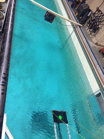
2.2. Data Acquisition and Experimental Setup

2.2.1. Data Acquisition and Image Processing

Two types of experiments are conducted to empirically measure the effect of water surface on the laser beam’s ray-path geometry. The goal of the first type of experiments is to provide wind speed and wave spectrum conditions similar to the water surface models described in Section 2.1. Wind over the water tank surface is generated using an industrial fan and wind speed is measured with an anemometer (Digital Tools Mini anemometer). To characterize the spectrum of the fan-generated capillary-gravity waves, water surface elevation is measured with a capacitive wave staff (Ocean Sensor Systems OSSI-010-002) at a sampling rate of 30 Hz.

The goal of the second type of experiments is to characterize the interaction of the laser beam with different water surface conditions using the optical detector array designed at the University of New Hampshire Center for Coastal and Ocean Mapping [29,30]. The optical detector array consists of a 6 × 6 photodiode array (Thorlabs PD1A) arranged in a planar square grid with dimensions of 0.25 m × 0.25 m. The spacing between the photodiodes is kept at 0.05 m to avoid optical cross talk between the elements [30]. Each photodiode is mounted in a clear acrylic waterproof housing. To increase the dynamic range, the photodiodes are connected via SubMiniature-A (SMA) cables to a reverse bias circuitry, which supplies a reverse bias voltage of 5 Volts. The detector array intersects the refracted laser beam and samples the light field at a sampling rate of 20 Hz using 10-bit (0-1023 digital counts) analog-to-digital converters. The output of the detector array is a 6 × 6 image. The laser beam centroid is calculated by using image moment invariants algorithm with sub-pixel accuracy.

Image moment invariant algorithm is an image processing technique that reveals information regarding the symmetry of a given image [31]. The moments of images algorithm are calculations of the weighted average of the image intensities as:

$$M_{pq}=\frac{1}{S}{\displaystyle \sum }_{i,j}{\left(x_i-x_o\right)}^p{\left(y_j-y_o\right)}^q{I}_{i,j}$$

(20)

where $M_{pq}$ is the image moment invariant with $p$ and $q$ are index values ($p$ = 1, 2, 3 and $q$ = 1, 2, 3), $x_o$ and $y_o$ are the index locations of the pixel of maximum intensity, $I$ is the pixel intensity, $S$ is the summation of pixel intensities, that is, $S={\displaystyle \sum }_{i,j}{I}_{i,j}$, and $i$ and $j$ are the number of pixels along the x- and y-directions. The image centroids, $\overline{x}$ and $\overline{y}$, which are used to compare the simulated and empirical laser beam centroids, are calculated as:

$$\left\{\overline{x},\overline{y}\right\}=\left\{\frac{M_{12}}{M_{11}} ,\frac{M_{21}}{M_{11}}\right\}$$

(21)

In this study, the image moment invariant algorithm is used to characterize the digitized laser beam image to known geometrical conditions, such as laser beam angle of incidence and beam diameter, through a calibration procedure. The calculated image centroids provide a measurement of the laser beam centroid shift as a function of the input parameters. Similar to the Monte Carlo ray-tracing simulations, variation of the image centroid locations is compared to a reference still water surface condition in order to measure the water surface refraction deviation when the water surface is disturbed by wind.

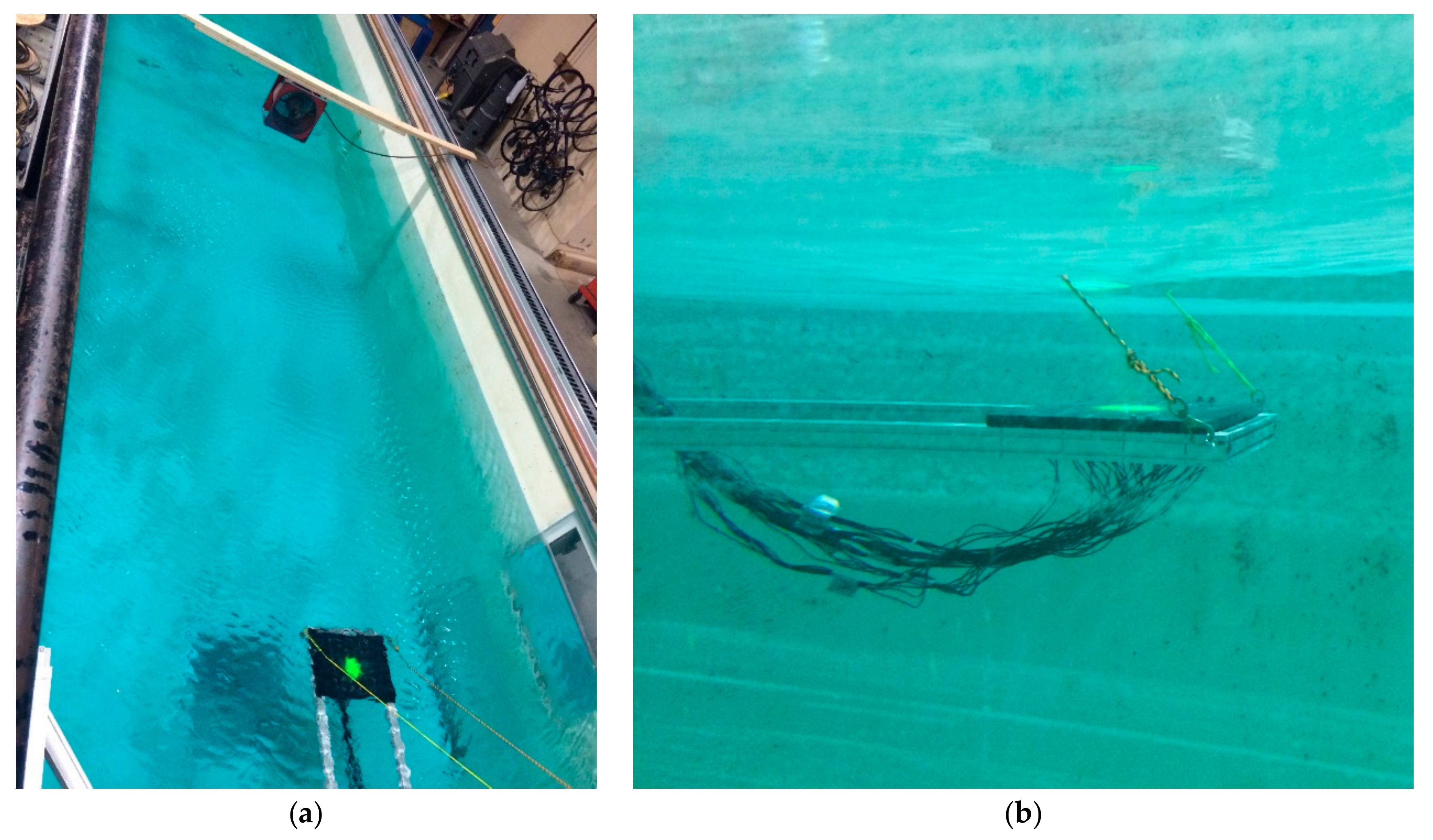
2.2.2. Experimental Setup

The empirical experiments were conducted in University of New Hampshire’s Ocean Engineering facilities using a wave tank (36.5 m long, 3.6 m wide and 2.4 m deep) (Figure 5a). Wind speed and water surface elevation data were collected at distances from 3.5 m to 8.5 m away from the industrial fan at 1 m increments. The positioning for data collection was provided using an actuated tow carriage with positioning accuracy of 0.01 m. A 5-min window sample was collected for statistical analysis at each configuration in order to capture a significant number of wave crests (more than 100 samples). The optical detector array was mounted on 80/20 aluminum frames to the tow carriage with an L-frame configuration and oriented horizontally to face upwards towards the water surface (Figure 5a). The modularity of the setup allowed geometrical changes in the configuration of the mount required to collect data at changing incidence angles. The detector array was submerged to a depth of 0.25 m below the water surface to minimize the scattering and absorption effects as described in Section 2.2 (Figure 5b). A 5 mW continuous wave laser pointer was mounted to the tow carriage at a height of 4 m. A plano-concave 75 mm focal length lens was used to expand the laser beam footprint diameter to 0.25 m on the water surface, which was limited mainly by the dimensions of the detector array. The laser beam incidence angle was varied from 0° to 20°, specifically, (0°, 10°, 15° and 20°). The laser beam image data obtained from the optical detector array were collected for 20 s at 20 Hz, that is, 400 frames were recorded at each configuration. The output of the optical detector array at two consecutive time steps in the same experimental configuration ($\theta$ = 15° and distance from the fan is 3.5 m) under disturbed water surface conditions is demonstrated in Figure 6a,b. The optical detector array allows the changes in the laser centroid location as well as the focusing and defocusing effect caused by the surface waves to be observed [2] Video S2.

3. Results

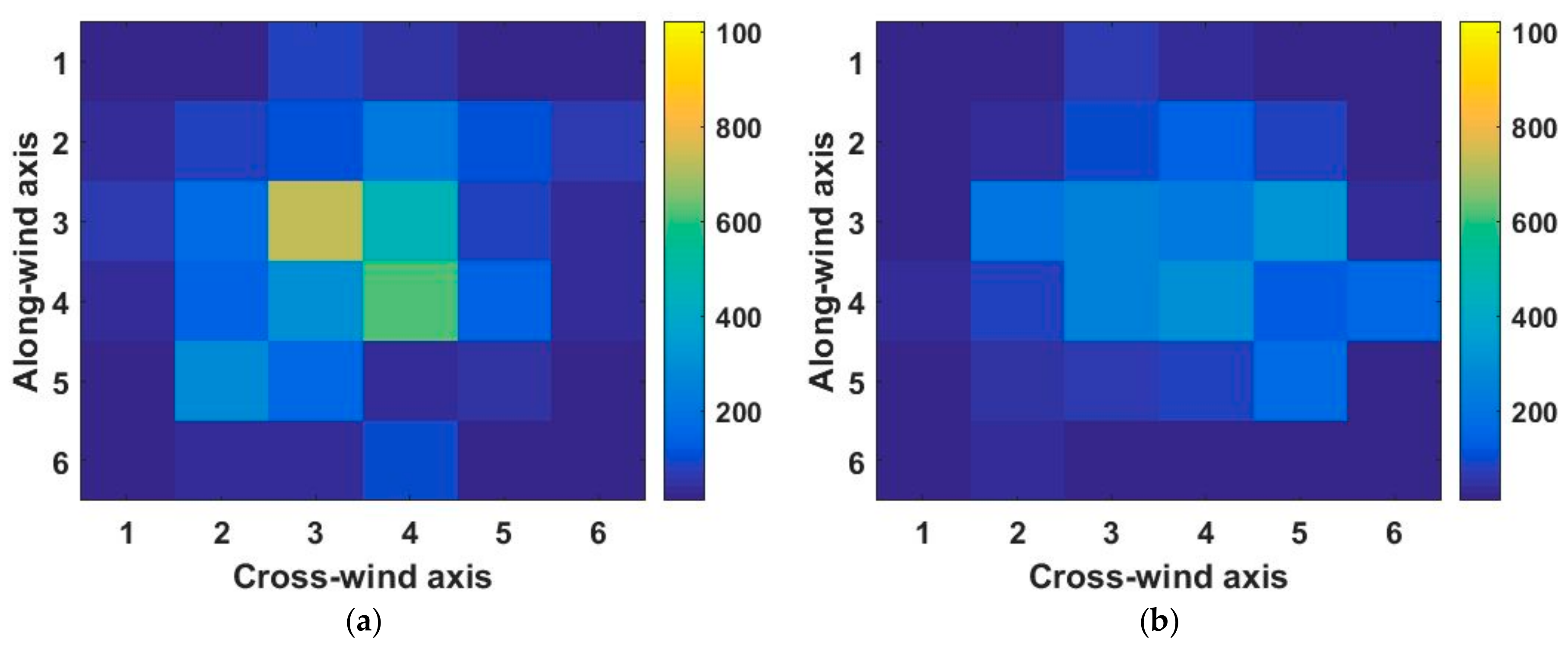
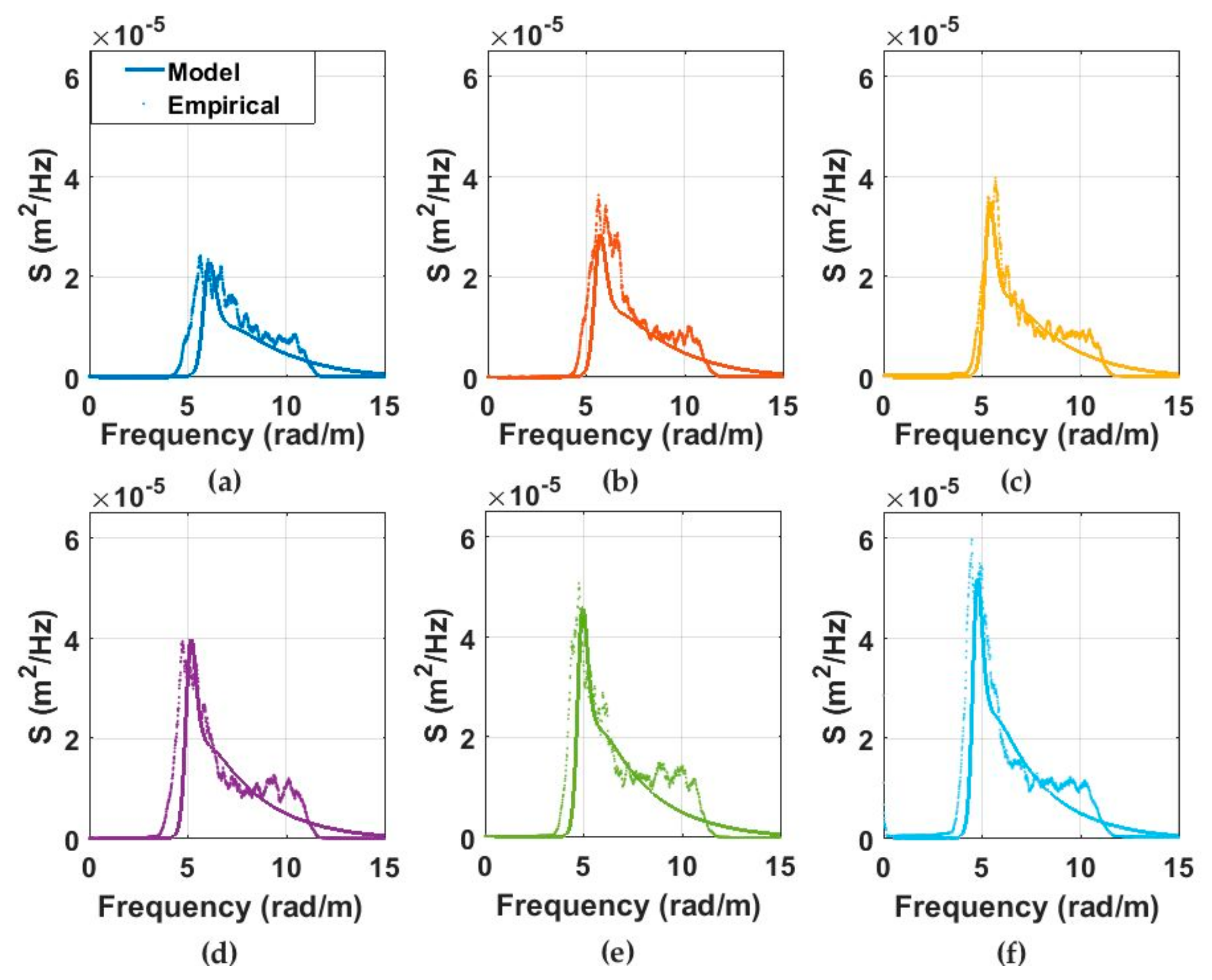
3.1. Wave Spectrum Results

The wave-staff measurements provided time-series of wave elevation data. Using Fourier Transform techniques, wave-staff measurements were processed to obtain the experimental wave spectrum.

Table 2. Key parameters obtained from the capacitive wave staff measurements.

Distance Downwind (m)	3.5	4.5	5.5	6.5	7.5	8.5
Peak Frequency (Hz)	5.6	5.5	5.3	4.6	4.4	4.3
Peak Wavelength (m)	0.050	0.051	0.055	0.074	0.080	0.085
Significant Wave Height (m)	0.008	0.010	0.011	0.009	0.009	0.009

summarizes the key parameters obtained from the capacitive wave staff measurements that include peak frequency, wavelength and significant wave height, calculated as average of the highest one-third of the waves, for each dataset.

The results show that the peak frequency decreases linearly (${\mathrm{R}}^2$ = 0.93) as the distance from the fan increases within the tested range. This decrease in the peak frequency indicates that the wavelengths increase linearly with increasing fetch. Also, the frequency content of the waves remains relatively constant for all distances within 6–10 Hz range. This constant frequency content shows that the capillary waves with small amplitude and relatively high frequency content are present in all cases. The shoulder effect observed between 10–12 Hz region, that is, slight increase in power spectrum amplitude, is attributed to the noise in the signal as it approaches the limit of the sensors measurement range of waves less than 0.002 m in height. The significant wave height also increases until 5.5 m and then decreases to 0.009 m and stays constant.

In order to relate the wave conditions in laboratory setting to real-world capillary-gravity wave conditions, a fully-developed Apel spectrum model is fitted to the experimental wave spectrum results. The fully developed Apel spectrum was chosen under the assumption that in real-world survey conditions, capillary-gravity waves almost always will be fully developed, that is, the waves are not limited by fetch. As demonstrated in [32], small waves in the capillary-gravity wave regimes are fully developed by a fetch of 30 m, a distance easily achieved even in near shore applications. Accordingly, an Apel wave spectrum model with a fetch of 30 m was fitted to the experimental spectrum (Figure 7). These models were then used in the air-water interface modeling in the Monte Carlo ray tracing simulations and the results were directly compared to the empirical measurements.

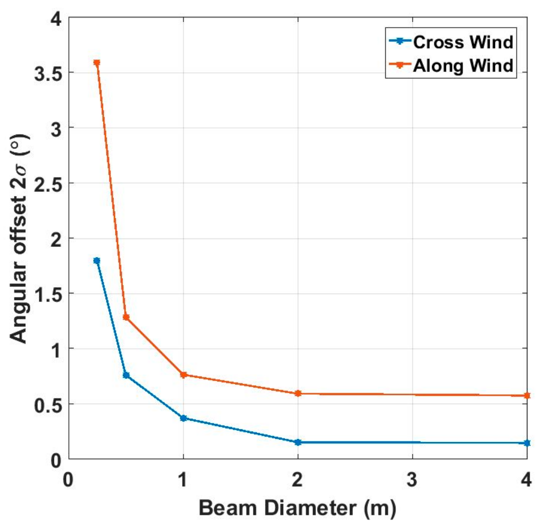
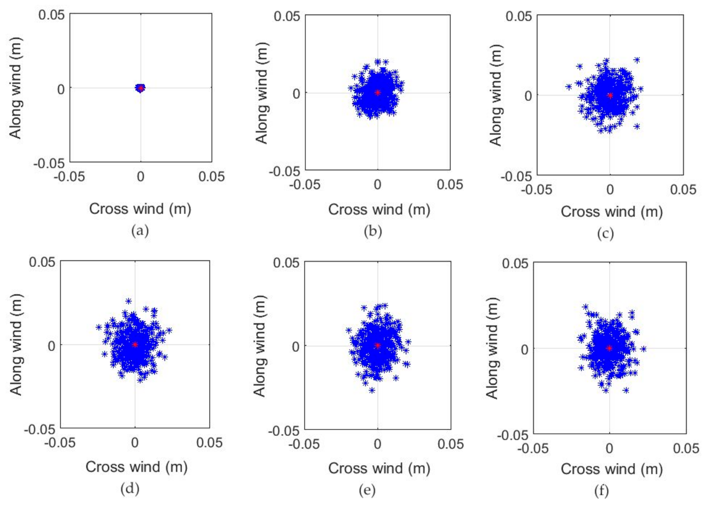
3.2. Monte Carlo Simulation Results

Using Monte Carlo simulations, it is possible to quantify the effect of wind speed, laser beam incidence angle and laser beam footprint diameter on the variation of a laser beam centroid in the along-wind (axis parallel to the direction of wind) and cross-wind (axis perpendicular to the direction of wind) directions (

Table 3. Refraction angle standard deviations ($2\sigma$) in the along-wind and cross-wind directions as obtained from Monte Carlo simulations for laser beam diameter of 0.25 m.

Laser Beam Incidence Angle (°)
Wind Speed (m/s)	Along-wind Direction					Cross-Wind Direction
	0°	5°	10°	15°	20°	0°	5°	10°	15°	20°
2	2.67°	2.49°	2.66°	2.99°	3.27°	2.02°	2.08°	2.00°	1.76°	1.68°
2.5	2.84°	2.74°	2.94°	3.23°	3.39°	2.03°	2.25°	2.04°	1.83°	1.72°
3	3.12°	2.93°	3.11°	3.47°	3.68°	2.29°	2.14°	2.09°	1.87°	1.80°
3.5	3.05°	3.12°	3.23°	3.53°	4.12°	2.27°	2.19°	2.03°	1.80°	1.75°
4	3.40°	3.52°	3.55°	3.84°	4.12°	2.25°	2.24°	1.99°	1.75°	1.75°
5.25	4.11°	3.79°	4.21°	4.52°	4.80°	2.44°	2.10°	2.05°	1.79°	1.64°

). The ray tracing results conducted with a laser beam diameter of 0.25 m indicate that the beam refraction angle standard deviation shows a linear pattern with wind speed in the along-wind direction (the lowest ${\mathrm{R}}^2$ = 0.95 at 0° incidence angle). In addition, the along-wind direction refraction angle deviation is positively correlated with the laser beam incidence angles. The maximum average incidence angle variation is observed for the 20° incidence angle results with 3.9°. These results indicate that ALB systems with circular or elliptical scanning patterns and off-nadir angles and that range between 15° to 20° are expected to have higher refraction error uncertainty in the along-wind direction than ALB systems with rectilinear scanning patterns, the off-nadir angles of which are smaller. In the cross-wind direction, no correlation was observed between the refraction angle standard deviation and the wind speed. The laser beam refraction angle standard deviations showed a constant pattern with respect to wind speed.

Additional sets of simulations were conducted in order to evaluate the effect of varying laser beam footprint diameter on the variation of the refraction angle. The simulation results conducted at a 15° incidence angle show that the larger diameter beams result in less variation in the refraction angle in the along-wind direction (Figure 8). These results verify the findings presented in [18] which state that the wave refraction error is higher for smaller diameter beam footprints than larger diameter beam footprints.

Additional simulations were conducted for a range of laser beam footprint diameters that are generated by commercial ALB systems (0.25 m, 0.5 m. 1 m, 2 m and 4 m) with wind speeds of 2 m/s, 2.5 m/s, 3 m/s, 3.5 m/s, 4 m/s and 5.25 m/s and the beam incidence angles ranging from 0$°$ to 20$°$ at 5$°$ intervals. The results were averaged to examine the effect of beam diameter on the along-wind and cross-wind refraction angle deviation (Figure 9).

The results in Figure 9 show that the variation in refraction angle for both the along-wind and cross-wind decreases with increasing beam diameters. The variation of the refraction angle in the along-wind direction is higher than in the cross-wind direction. It is observed that for ALB systems operating with a laser beam diameter of 2 m or larger, refraction angle variations in the along-wind and cross-wind directions stay relatively constant.

3.3. Empirical Results

An optical detector array was used to collect laser beam footprint images under a variety of water surface and laser beam geometry conditions, including varying wind speed, laser beam incidence angle and distances between the laser beam footprint and the fan. The refraction angle variation was assessed by using image centroid calculations described in Section 3.2. A total of 400 image frames were collected and statistically analyzed to estimate the refraction angle. Data sets were collected for laser beam incidence angles of 0°, 10°, 15° and 20°. The variation in the laser beam centroid location was calculated as a result of interaction with the water surface. The results are compared to the reference centroid calculations conducted using a still water surface condition (Figure 10).

The results in Figure 10 indicate that the standard deviation ($2\sigma$) of the beam center for the wind-driven water surface cases is around $\pm$0.015 m at a depth of 0.25 m, which is approximately an order of magnitude larger than the standard deviation observed in the still water case (the maximum error is ~0.00086 m at $2\sigma$ for along and cross-wind directions). The results also showed that the laser beam center fluctuates slightly more in the along-wind direction than the cross-wind direction due to the nature of the wave spreading in the wave tank. The observed shifts in the laser beam center of concentration is converted to refraction angles. The standard deviation values of the refraction angles obtained from the empirical measurements are demonstrated in

Table 4. Refraction angle standard deviations ($2\sigma$) in the along-wind and cross-wind directions as obtained from empirical measurements for a laser beam diameter of 0.25 m.

Wind Speed (m/s)	Laser Beam Incidence Angle (°)
	The Along-Wind Direction				Cross-Wind Direction
	0°	10°	15°	20°	0°	10°	15°	20°
2	3.33°	3.42°	3.24°	3.61°	3.11°	3.13°	3.00°	3.00°
2.5	3.78°	3.43°	3.61°	3.54°	3.73°	3.20°	3.55°	3.09°
3	3.58°	3.55°	3.73°	3.92°	3.50°	3.38°	3.48°	3.49°
3.5	3.64°	3.56°	3.98°	3.94°	3.55°	3.48°	3.32°	3.23°
4	3.68°	3.80°	3.73°	4.21°	3.67°	3.36°	3.25°	3.69°
5.25	4.04°	3.88°	4.33°	4.58°	4.68°	3.15°	3.55°	3.30°

.

The empirical refraction angle calculations showed that the along-wind refraction angle standard deviation is linearly correlated with the wind speed (the lowest ${\mathrm{R}}^2$ = 0.84 is observed for a 15° incidence angle, considering the standard deviation result for the case of a 0° incidence angle and a 2.5 m/s wind speed as an outlier). However, no correlation with wind speed was observed in the cross-wind directions. Comparison between the results obtained from the Monte Carlo simulations and the empirical measurements shows similar trends and values for the refraction angle standard deviation, especially in the along-wind direction. The refraction angle standard deviation is linearly dependent on the wind speeds in both simulations and empirical measurements. The maximum average standard deviation value of 3.9° is observed for 20° incidence angle, which is approximately the same with the simulation results (3.8° in simulations). Similar to the simulation results, the refraction angle standard deviation in cross-wind direction does not show a correlation to wind speed or incidence angle. The main difference between the simulation and empirical results were observed in the numerical values of the refraction angle standard deviation in the cross-wind direction. The cross-wind standard deviation values obtained from the empirical measurements is on average approximately 1.5° higher than in Monte Carlo simulations.

4. Discussion

The results obtained in this study can be used to estimate the THU and TVU components at various depths. According to IHO, the maximum allowable THU and TVU in Order 1b standards are defined as:

$$THU=5+0.02\ast depth$$

(22)

$$TVU= \pm \sqrt{{\left(0.5\right)}^2+{\left(0.013\ast depth\right)}^2}$$

(23)

In order to verify the NOAA forensic analysis that ALB surveys can be considered IHO S-44 order 1b [11], the THU and TVU values are estimated for ALB survey conditions with a wind speed of 5.25 m/s at 20° incidence angle (

Table 5. Comparison of the estimated THU and TVU values (2$\mathsf{\sigma }$) obtained from the Monte Carlo simulations based on the empirical refraction angle standard deviation values obtained from 20° incidence angle and 5.25 m/s wind speed.

Depth (m)	THU (m)	IHO-1b THU(m)	TVU (m)	IHO-1b TVU (m)
1	0.10	5.02	0.03	0.50
2	0.21	5.04	0.05	0.50
3	0.32	5.06	0.08	0.50
4	0.42	5.08	0.11	0.50
5	0.52	5.10	0.13	0.50
6	0.63	5.12	0.16	0.51
7	0.74	5.14	0.19	0.51
8	0.84	5.16	0.21	0.51
9	0.95	5.18	0.24	0.51
10	1.05	5.20	0.27	0.52

). A Monte Carlo simulation was conducted to calculate depth that range from 1 m to 10 m and the horizontal displacement of the laser beam using 10,000 realizations. The empirical the along-wind and cross-wind refraction angles demonstrated in Table 4 were used to calculate the TVU and THU in the Monte Carlo simulations. Accordingly, the THU values were calculated as follows:

$$THU=2\ast std\left(depth\ast \tan \left(\theta +\Delta \theta \right)\right)$$

(24)

The extended ray paths due to the refraction angle standard deviation are calculated as:

$$r_{ext}=\frac{depth}{\cos \left(\theta +\Delta \theta \right)}$$

(25)

where ${\mathrm{r}}_{\mathrm{ext}}$ is the extended ray path due to the refraction angle standard deviation. Then, the TVU values were calculated by multiplying the laser ray path with cosine of the incidence angle as:

$$TVU=2\ast std\left(r_{ext}\ast \cos \theta \right)$$

(26)

The results in Table 5 show the estimated horizontal and vertical uncertainty results estimated from the Monte Carlo simulations as well as the maximum allowable THU and TVU as defined by IHO Order 1-b. The results indicate that both estimated THU and TVU values are within the IHO Order-1b standards. It is also observed that the maximum allowable TVU is more stringent than the maximum allowable THU. For example, the calculated TVU value (2$\sigma$) at 10 m depth is ~0.27 m whereas the IHO Order-1a specification is ~0.52 m. These findings are critical in a sense that it demonstrates the water surface contribution to the TPU budget as a function of depth. In addition, the remaining uncertainty tolerance is quantified for other uncertainty mechanisms that are not included in this paper, for example, trajectory, scanning angle, water column scattering and seafloor reflection.

The results presented in this paper can also be generalized with respect to wind speed, laser beam incidence angle and laser beam footprint size on the water surface. The refraction angle variation in the along-wind direction is linearly correlated with the wind speeds (i.e., $\Delta {\theta }_{aw}=a_{a}U+b_a$), whereas the refraction angle variation in the cross-wind direction can be approximated as a constant ($\Delta {\theta }_{cw}=b_c)$. In addition, the refraction angle variation in both across-wind and the along-wind directions increase with larger laser beam incidence angle. Overall, the refraction angle standard deviations (2$\mathsf{\sigma }$) in the along-wind and cross-wind directions with respect to wind speed and beam incidence angle is modeled as:

$$\Delta {\theta }_{aw}=\left(0.003\theta +0.4193\right)w+0.00276\theta +1.6208$$

(27)

$$\Delta {\theta }_{cw}=\left(-0.0009\theta +0.0063\right)w-0.00281\theta +2.3$$

(28)

where $w$ is the wind speed. The results obtained can also be extended to systems that use different beam footprint diameters by using a correction factor. Based on the results presented in Figure 10, the correction factors for the along-wind and cross-wind refraction angle standard deviation is given as:

$$C_{F-aw}=0.2897\ast D^{-0.641}$$

(29)

$$C_{F-cw}=0.227\ast D^{-0.951}$$

(30)

For laser beam foot print diameters that range between $0.25<\mathrm{D}\le 4$.

Although the results for the along-wind directions agreed with the simulation and empirical results, the cross-wind refraction angle standard deviation values are higher in the empirical measurements than in the simulation results. In addition, in the Monte Carlo simulations, the along-wind refraction angle standard deviation values are higher than the cross-wind refraction angle standard deviation values (Table 3) when compared to empirical results (Table 4). This was attributed to the differences in the data resulting from the simulations conducted with a set of approximations and the laboratory environment. In the empirical measurements, the waves might have reflected off the wall and changed direction until they intersected the laser beam footprint, resulting in a different wave spreading pattern. These off-directional waves might have contributed in the larger cross-wind refraction angles observed in the empirical data than in the Monte Carlo ray tracing simulations. In the Monte Carlo simulations, the surface waves follow a more uniform pattern than in the empirical measurements, which results in along-wind refraction angle standard deviation values that are higher than the cross-wind refraction angle standard deviation values. Another factor that could result in the differences in the simulation and empirical results is the method of centroid calculation in both methods. In the simulation results demonstrated in Table 3, there is a decreasing trend in the cross-wind refraction angle standard deviation values with incidence angles whereas there is no such trend in the empirical results (Table 4). Since the laser beam centroid calculation relies on the laser‘s ray-path geometry and energy, a potential difference in the results may occur if surface wave models in the Monte Carlo simulations do not exactly represent the empirical waves.

The sub-pixel accuracy algorithm used in the image processing methods enhanced the error resolution in the empirical measurements. Using the optical detector array, the centroid estimation error was measured to be 0.00086 m (2$\sigma$) at z = 0.25 m for the along-wind and cross-wind directions as shown in Figure 10a. This translates into refraction angle measurement error of ~0.2° (2$\sigma$) in the along-wind and cross-wind directions. Although the spacing between the photodiodes in the optical detector array is configured to be 0.05 m, sub-pixel accuracy algorithm allows to calculate the positioning errors at a higher resolution.

Although there is good agreement between the simulated and the empirical measurements, the results presented in this study should be evaluated as preliminary due to the limited number of wind speeds used in the simulation and experiments. In the empirical measurements, the main limitation was the fan power that provided the wind output to generate the capillary-gravity waves. However, in survey conditions higher wind speed values are likely to occur. At wind speeds greater than 5.25 m/s, the linear trend observed between wind speed and the along-wind refraction angle standard deviation may not be valid. Instead, a nonlinear trend may be observed. Therefore, care should be taken in extrapolating the results provided in this study to wind speeds that are larger than 5.25 m/s.

Another important contribution of the study is regarding the effect of ALB hardware on the measurement uncertainty. It is observed that larger laser beam diameters result in less refraction angle variation due to the laser beam interaction with the small wind waves. The decrease in refraction error for larger laser beam footprints is attributed to an averaging effect, that is, the total number of wave crests within the footprint is large enough that the majority of the laser rays is still refracted along the direction predicted by the still water assumption. This means that for topo-bathymetric lidar systems that use smaller footprints than conventional bathymetric lidar systems, the measurement uncertainties can be greater. Another significant observation is found for the ALB systems that use circular or elliptical scanning patterns whose off-nadir angles range between 15–20°. The refraction angle variation at this range is found to be greater in circular or elliptical scanning patterns than the ALB systems that use rectilinear scanning patterns with smaller off-nadir angle.

Although this study provided a method to decouple the uncertainties caused by the air-water interface, further investigation is needed to produce a comprehensive ALB uncertainty model that includes the effects of uncertainties caused by both hardware and environmental uncertainties. These uncertainties include the aircraft trajectory, scanning unit, atmospheric effects, scattering in the water column and turbidity as well as seafloor contributions. The results obtained from the variation of these uncertainty parameters can be used in a look-up table to report horizontal and vertical TPU on per-pulse basis.

5. Conclusions

In this study, the contribution of the air-water interface on the ALB measurement uncertainty is assessed. Monte Carlo ray tracing simulations along with empirical measurements were used to measure refraction angle variation as a result of laser beam interaction with the air-water interface. The results show that the wind speed is a dominant parameter that affects the refraction angle standard deviation. In addition, the wind direction has an impact on the wave refraction angle variation. The variation in the refraction angle in the direction parallel to the wind (the along-wind) is greater than in the orthogonal direction (cross-wind). Good agreement between the Monte Carlo simulations and empirical results was found. In both approaches, the refraction angle standard deviations ($2\mathsf{\sigma }$) in the along-wind direction vary between 3–5° when the variations in wind speed, laser beam footprint size and the laser beam incidence angle are taken into account.

The results also suggest that different hardware configurations used by different lidar manufacturers may result in different uncertainty measurements. ALB systems with circular or elliptical scanning patterns that have off-nadir angles ranging between 15° and 20° are expected to have higher refraction error uncertainty in the along-wind direction than ALB systems with rectilinear scanning patterns, the off-nadir angles of which are smaller. Also, smaller beam footprint systems typically employed by the topo-bathymetric lidar systems tend to have higher refraction angle variation when the dominant wave mechanism is capillary-gravity waves. The results of this study can be used to estimate water surface contribution to the overall TPU budget and provide a baseline for look-up tables that can be used in bathymetric lidar TPU reporting.

References

1. Guenther, G. Airborne Laser Hydrography: System Design and Performance Factors; NOAA Professional Paper Series; NOAA: Silver Spring, MD, USA, 1985. [Google Scholar]
2. Wang, C.K.; Philpot, W.D. Using airborne bathymetric lidar to detect bottom type variation in shallow waters. Remote Sens. Environ. 2007, 106, 123–135. [Google Scholar] [CrossRef]
3. Eren, F.; Pe’eri, S.; Rzhanov, Y.; Ward, L. Bottom characterization by using airborne lidar bathymetry (ALB) waveform features obtained from bottom return residual analysis. Remote Sens. Environ. 2018, 206, 260–274. [Google Scholar] [CrossRef]
4. Peeri, S.; Gardner, J.V.; Ward, L.G.; Morrison, J.R. The seafloor: A key factor in lidar bottom detection. IEEE Trans. Geosci. Remote Sens. 2011, 49, 1150–1157. [Google Scholar] [CrossRef]
5. Riegl VQ-880-G Laser Scanner System for Topo-Bathymetric Surveying with New Optional IR Laser Scanner Channel. Available online: http://www.3dlasermapping.com/wp-content/uploads/2015/02/3DLM-RIEGL-User-Conference_VQ-880-GOverview_Rg_PDF_low.pdf (accessed on 20 December 2017).
6. Pan, Z.; Glennie, C.; Hartzell, P.; Fernandez-Diaz, J.C.; Legleiter, C.; Overstreet, B. Performance assessment of high resolution airborne full waveform LiDAR for shallow river bathymetry. Remote Sens. 2015, 7, 5133–5159. [Google Scholar] [CrossRef]
7. Guenther, G.C.; Cunningham, A.G.; Larocque, P.E.; Reid, D.J.; Service, N.O.; Highway, E.; Spring, S. Meeting the Accuracy Challenge in Airborne Lidar Bathymetry. In Proceedings of the 20th EARSeL Symposium: Workshop on Lidar Remote Sensing of Land and Sea, Dresden, Germany, 16–17 June 2000. [Google Scholar]
8. Mobley, C.D. Light and Water: Radiative Transfer in Natural Waters; Academic Press: Cambridge, MA, USA, 1994. [Google Scholar]
9. Lockhart, C.; Lockhart, D.; Martinez, J. Total Propagated Uncertainty (TPU) for hydrographic lidar to aid objective comparison to acoustic datasets. Int. Hydrogr. Rev. 2008, 9, 19–27. [Google Scholar]
10. International Hydrographic Organization (IHO). IHO Standards for Hydrographic Surveys: Special Publication No. 44, 5th ed.; IHO: Monaco, 2008. [Google Scholar]
11. Imahori, G.; Ferguson, J.; Wozumi, T.; Scharff, D.; Pe’eri, S.; Parrish, C.E.; White, S.A.; Jeong, I.; Sellars, J.; Aslaksen, M. A Procedure for Developing an Acceptance Test for Airborne Bathymetric Lidar Data Application to NOAA Charts in Shallow Waters; National Oceanic and Atmospheric Administration (NOAA) National Ocean Survey (NOS) Technical Memorenadom CS 32; NOAA: Silver Spring, MD, USA, 2013. [Google Scholar]
12. Krekov, G.M.; Krekova, M.M.; Shamanaev, V.S. Laser sensing of a subsurface oceanic layer I Effect of the atmoshpere and wind-driven sea waves. Appl. Opt. 1998, 37, 1589–1595. [Google Scholar] [CrossRef] [PubMed]
13. McLean, J.W.; Freeman, J.D. Effects of ocean waves on airborne lidar imaging. Appl. Opt. 1996, 35, 3261–3269. [Google Scholar] [CrossRef] [PubMed]
14. Tulldahl, H.M.; Steinvall, O.K. Simulation of sea surface wave influence on small target detection with airborne laser depth sounding. Appl. Opt. 2004, 43, 2462–2483. [Google Scholar] [CrossRef] [PubMed]
15. Mclean, J.W. Modeling of Ocean Wave Effects for Lidar Remote Sensing. SPIE 1302, Ocean Optics X, 1 September 1990. In Proceedings of the Technical Symposium on Optics, Electro-Optics, and Sensors, Orlando, FL, USA, 16–20 April 1990. [Google Scholar] [CrossRef]
16. Steinvall, O.V.E.; Koppari, K. Depth Sounding Lidarperformance and Models. SPIE 2748, Laser Radar Technology and Applications, 26 June 1996. In Proceedings of the Aerospace/Defense Sensing and Controls, Orlando, FL, USA, 8–12 April 1996. [Google Scholar]
17. Westfeld, P.; Maas, H.G.; Richter, K.; Weiss, R. Analysis and correction of ocean wave pattern induced systematic coordinate errors in airborne LiDAR bathymetry. ISPRS J. Photogramm. Remote Sens. 2017, 128, 314–325. [Google Scholar] [CrossRef]
18. Karlsson, T. Uncertainties Introduced by the Ocean Surface when Conducting Airborne Lidar Bathymetry Surveys. Master Thesis, Lund Institute of Technology, Lund, Sweden, 9 December 2011. [Google Scholar]
19. Dean, R.; Dalrymple, R. Water Wave Mechanics for Engineers and Scientists; Prentice Hall: Upper Saddle River, NJ, USA, 1984. [Google Scholar]
20. Mobley, C.D. Modeling Sea Surfaces: A Tutorial on Fourier Transform Techniques. Available online: http://www.oceanopticsbook.info/view/references/publications#mobley_2016 (accessed on 12 December 2017).
21. Apel, J.R. An improved model of the ocean surface wave vector spectrum and its effects on radar backscatter. J. Geophys. Res. 1994, 99, 16269–16291. [Google Scholar] [CrossRef]
22. Hasselmann, K.; Olbers, D.J. Measurements of Wind-Wave Growth and Swell Decay during the Joint North Sea Wave Project (JONSWAP). Dtsch. Hydrogr. Z. 1973, A, 95. [Google Scholar]
23. Elfouhaily, T.; Chapron, B.; Katsaros, K.; Vandemark, D. A unified directional spectrum for long and short wind-driven waves. J. Geophys. Res. Ocean. 1997, 102, 15781–15796. [Google Scholar] [CrossRef]
24. Klinke, J.; Jahne, B. 2D Wave Number Spectra of Short Wind Waves—Results from Wind Wave Facilities and Extrapolation to the Ocean. In Proceedings of the SPIE, Optics of the Air-Sea Interface: Theory and Measurement, San Diego, CA, USA, 22–22 July 1992. [Google Scholar]
25. Preisendorfer, R.W.; Mobley, C. Albedos and glitter patterns of a wind-roughened sea surface. J. Phys. Oceanogr. 1986, 16, 1293–1316. [Google Scholar] [CrossRef]
26. Demirbilek, Z.; Linwood, C. Coastal Engineerin Manual; Manual Number: EM 1110-2-1100; U.S. Army Corps of Engineers (USACE): Washington, DC, USA, 2002. [Google Scholar]
27. Mitsuyasu, H.; Tasai, F.; Suhara, T.; Mizuno, S.; Ohkusu, M.; Honda, T.; Rikiishi, K. Observations of the directional spectrum of ocean waves using a coverleaf buoy. J. Phys. Oceanogr. 1975, 5, 750–760. [Google Scholar] [CrossRef]
28. Greve, B. Reflections and Refractions in Ray Tracing. Available online: https://graphics.stanford.edu/courses/cs148-10-summer/docs/2006--degreve--reflection_refraction.pdf (accessed on 5 November 2017).
29. Eren, F.; Pe’eri, S.; Rzhanov, Y.; Thein, M.; Celikkol, B. Optical detector array design for navigational feedback between unmanned underwater vehicles (UUVs). IEEE J. Ocean. Eng. 2016, 41, 18–26. [Google Scholar] [CrossRef]
30. Eren, F.; Pe’eri, S.; Thein, M.W.; Rzhanov, Y.; Celikkol, B.; Swift, M.R. Position, orientation and velocity detection of Unmanned Underwater Vehicles (UUVs) using an optical detector array. Sensors 2017, 17, 1741. [Google Scholar] [CrossRef] [PubMed]
31. Rzhanov, Y.; Eren, F.; Thein, M.-W.; Pe’eri, S. An Image Processing Approach for Determining the Relative Pose of Unmanned Underwater Vehicles. In Proceedings of the OCEANS 2014—TAIPEI, Taipei, Taiwan, 7–10 April 2014; pp. 1–4. [Google Scholar] [CrossRef]
32. Zhang, X. Capillary–gravity and capillary waves generated in a wind wave tank: Observations and theories. J. Fluid Mech. 1995, 289, 51–82. [Google Scholar] [CrossRef]
Figure 1. The schematic of laser beam interaction with (a) Gravity waves with wavelengths larger than the laser beam footprint; (b) Capillary waves with wavelengths smaller than the laser beam footprint. The arrows denote the surface normal of the wave facets.
Remotesensing 10 00453 g001
Figure 2. Wave spectrum, spreading function and directional spectrum for an Apel wave spectrum model with wind speed U = 5 m/s and fetch length of 5.5 m. (a) 1-D Apel wave spectrum; (b) Cos-2s spreading function; (c) Directional spectrum.
Remotesensing 10 00453 g002
Figure 3. 3D water surface model triangulated by Delaunay triangulation.
Remotesensing 10 00453 g003
Figure 4. The directional vectors for the transmitted ray through the water surface, incident ray ( s 1 ), refracted ray ( s 2 ) and the water surface normal vector ( N s u r f ). The axis conventions are also demonstrated.
Remotesensing 10 00453 g004
Figure 5. Experimental setup at the University of New Hampshire (UNH) Ocean Engineering laboratory. (a) The optical detector array and the industrial fan that creates a wind rippled water surface; (b) The optical detector array submerged into the water column at a depth of 0.25 m.
Remotesensing 10 00453 g005
Figure 6. Laser beam as intersected by the optical detector array at two consecutive time steps in the same experimental configuration, θ = 15° and distance from the fan is 3.5 m. (a) Image samples at t = Δ t ; (b) Image sampled at t = Δ t + 0.05 s.
Remotesensing 10 00453 g006
Figure 7. Experimental wave spectrum matched to fully developed capillary-gravity Apel wave spectrum model. Distance from the fan: (a) 3.5 m; (b) 4.5 m; (c) 5.5 m; (d) 6.5 m; (e) 7.5 m and (f) 8.5 m.
Remotesensing 10 00453 g007
Figure 8. The effect of laser beam footprint diameter on the refraction angle standard deviation in the along-wind direction for an off-nadir angle of 15°.
Remotesensing 10 00453 g008
Figure 9. The refraction angle deviation change with beam diameter for averaged wind speed and incidence angles.
Remotesensing 10 00453 g009
Figure 10. The laser beam centroid calculations shown for laser beam incidence angle of 15° with various wind speeds. (a) still surface (b) 2.5 m/s (c) 3 m/s (d) 3.5 m/s (e) 4 m/s (f) 5.25 m/s.
Remotesensing 10 00453 g010