kCCA Transformation-Based Radiometric Normalization of Multi-Temporal Satellite Images

Abstract

Radiation normalization is an essential pre-processing step for generating high-quality satellite sequence images. However, most radiometric normalization methods are linear, and they cannot eliminate the regular nonlinear spectral differences. Here we introduce the well-established kernel canonical correlation analysis (kCCA) into radiometric normalization for the first time to overcome this problem, which leads to a new kernel method. It can maximally reduce the image differences among multi-temporal images regardless of the imaging conditions and the reflectivity difference. It also perfectly eliminates the impact of nonlinear changes caused by seasonal variation of natural objects. Comparisons with the multivariate alteration detection (CCA-based) normalization and the histogram matching, on Gaofen-1 (GF-1) data, indicate that the kCCA-based normalization can preserve more similarity and better correlation between an image-pair and effectively avoid the color error propagation. The proposed method not only builds the common scale or reference to make the radiometric consistency among GF-1 image sequences, but also highlights the interesting spectral changes while eliminates less interesting spectral changes. Our method enables the application of GF-1 data for change detection, land-use, land-cover change detection etc.

1. Introduction

There is an increasing demand for image sequence analysis, because of the growing use of multi-sensor and multi-temporal remote sensing data to monitor the land-use and land-cover change (LUCC) and climate change, as well as to analyze the global resource environment [1,2,3,4]. A satellite image sequence is usually constructed from multi-temporal images generated by one common sensor or multiple sensors. Radiometric normalization is a fundamental method used in the pre-processing of satellite image sequence analysis, especially in the pre-processing of change detection [5]. Radiometric normalization can directly make use of the pixel values of an image to establish the corresponding transformation equation for each multi-spectral band in multi-temporal remote sensing data, without the request of any other parameters such as the atmospheric conditions when the remote sensing data obtained [6]. In such a context, radiometric normalization is called spectral alignment [7]. Radiometric normalization builds not only the common radiometric scale/reference but also the radiometric consistency among an image sequence.

Most radiometric normalization methods make use of the pseudo-invariant feature (PIF) to obtain the common scale among an image sequence (PIF)-based [5,8,9]. It is well-known that these invariant features—the targets whose spectral reflectance does not change over time, are necessary for the atmospheric normalization of temporal image sequences, and thus they are the basis of image sequence analysis [10]. All the PIF-based methods are linear, and they minimize the image radiometric differences caused by different acquisition conditions, such as atmospheric conditions, earth-sun distance, detector calibration, illumination angles, viewing angles and sensor oscillation [5,6,11,12,13].

The core problem of PIF-based methods is the selection of appropriate PIF points [13]. From simple to sophisticated, various PIF-based methods were developed for image normalization, such as the Ridge method [2,14,15,16], Simple image regression [4], Dark set-Bright set (DB) [17] and Automatic Scattergram Control Regression (ASAR) [18,19], etc. Specifically, Canty and Nielsen developed a powerful and widely used method, the iteratively reweighted multivariate alteration detection (iRMAD) transformation, which is invariant to linear and affine scaling. One advantage of this method is that only one parameter needs to be specified, i.e., the chi-squared percentile [20,21,22,23].

However, such a linear radiometric normalization cannot eliminate the nonlinear spectral differences, especially the surface reflectance differences [24]. In fact, beside PIFs, there are another two kinds of features/targets in image sequences. One kind of features/targets is the feature whose spectral reflectance changes regularly or expectably over time, such as vegetation growth. The other kind of features/targets is the feature whose spectral reflectance changes irregularly over time, such as city expansion and human activity trails. When these irregularly changed features are analyzed in an image sequence, the regularly changed features are the disturbances that need to be eliminated or attenuated by radiometric normalization. The changes caused by the growth of the vegetation are the most typical non-linear changes in radiometric value of image sequence. Especially, they may induce serious disturbance when the human induced changes are detected. Therefore, different spectral changes need different radiometric normalization methods. If the change detection involves the vegetation variation which needs to be preserved and enhanced, the impact from other features’ changes should be eliminated as much as possible.

Eliminating the effects of the regularly nonlinear spectral differences caused by seasonal variation of natural objects requires a nonlinear radiometric normalization method. Histogram matching is a commonly used nonlinear method, but it only uses global statistical information. Thus, it is less flexible and so difficult to adapt to specific applications [4,25].

In this paper, we propose a novel method of nonlinear radiometric normalization to extract nonlinear relationship between multi-temporal image-pairs. The proposed method is based on the kernel version of canonical correlation analysis (kCCA) [1,26,27,28,29,30,31], that consists of two steps. First, the image-pairs are quantitatively evaluated to extract the unchanged pixels whose Features are Nonlinear Invariant in kernel space (NIFs). Second, the nonlinear transformation of image-pairs is obtained from the nonlinear regression of the NIFs extracted previously. We will analyze the characteristics of NIFs distribution, nonlinear transformations and radiometric normalization results from different temporal image-pairs and compare the results with PIFs-based (CCA-based) method and histogram matching method. The PIFs-based method is derived from CCA of the spectral alignment of linear transformations, and the histogram matching is derived from statistical distribution models.

The paper is organized as follows: In Section 2, we describe the principle of the kernel version of CCA, as well as the selection of NIFs. Section 3 presents the test data and the experimental results, Section 4 is the discussion about the results. Section 5 we give the conclusion of the paper.

2. Relative Radiometric Normalization Based on kCCA Transformation

The proposed method contains two steps: the extraction of NIFs using kCCA and the use of NIFs to derive radiometric normalization. In this section, we review the kCCA transformation and how to extract NIFs based on it.

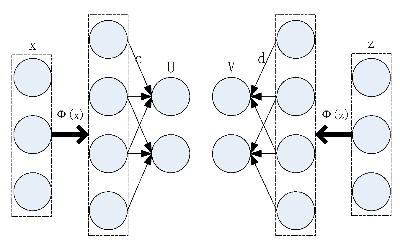
2.1. kCCA Transformation and NIFs Extraction

kCCA is the kernel version of CCA [7]. CCA is a multivariate feature extraction method that aims at finding the rotation of two sets of variables that maximizes their joint correlation [32]. In principle, CCA tends to select a group of representative indicators (linear combination of variables) from the two sets of random variables. These indicators express the correlation between the two sets of variables.

kCCA introduces the theory of kernel functions into CCA, which maps data from a low-dimension to a high-dimensional feature space. Each kernel function converts an n-dimensional inner product in low-dimensional space into an m-dimensional inner product in high-dimensional space. Let $\mathit{x},\mathit{z}\in R^n$, the nonlinear function $\mathsf{\varphi }\left(\mathit{x}\right)$ converts $R^n$ to $R^m$: $\mathit{x}\to \mathsf{\varphi }\left(\mathit{x}\right)$ ($n\ll m$), using the kernel function:

$$\mathit{k}\left(\mathit{x},\mathit{z}\right)=<\varphi \left(\mathit{x}\right),\mathit{\varphi }\left(\mathit{z}\right)>,$$

(1)

$<,>$ is the inner product, and $k\left(\mathit{x},\mathit{z}\right)$ is a kernel matrix [33,34]. It is not necessary to know the form and parameters of the nonlinear transformation function $\varphi \left(\mathit{x}\right)$ in advance. The kCCA method maps the target image and the reference image into high dimensional space in which their linear combination can be obtained. The canonical variable in high dimensional is defined as follows,

$$\mathit{U}={\mathit{c}}^{\mathit{T}}{\mathit{\phi }}_{\mathit{x}}\left(\mathit{x}\right),$$

(2)

$$\mathit{V}={\mathit{d}}^{\mathit{T}}{\mathit{\phi }}_{\mathit{z}}\left(\mathit{z}\right),$$

(3)

where $\mathit{x}$ represents the target image matrix. Each row of $\mathit{x}$ is a sample vector, and thus $\mathit{x}$ has size $n\times N$ where n is the number of bands and $N$ is the number of sample points of the image-pair. $\mathit{x}$ can be rewritten as ${\mathit{x}}_{n\times N}=\left({\mathit{x}}_1, {\mathit{x}}_2\cdots {\mathit{x}}_N\right)$ by column vectors ${\mathit{x}}_i$. $\mathit{z}$ represents the reference image matrix and similarly $\mathit{z}$ can be rewritten as ${\mathit{z}}_{n\times N}=\left({\mathit{z}}_1, {\mathit{z}}_2\cdots {\mathit{z}}_N\right)$. $\mathit{c}$ and $\mathit{d}$ are constant vectors of $R^m$. U denotes the linear combination of $\mathit{x}$ in the high-dimensional feature space; and V denotes the linear combination of $\mathit{z}$ in the high-dimensional feature space. The workflow of kCCA is shown in Figure 1. Similar to the solving process of linear correlation analysis, the first step is to solve $\mathit{c}$ and $\mathit{d}$ so that the correlation coefficients of the combined variables $\mathit{U}$ and $\mathit{V}$ are maximized.

To solve the vectors $\mathit{c}$ and $\mathit{d}$ in a lower dimensional space, $\mathit{c}$ and $\mathit{d}$ (of length m) are projected onto the vectors $\mathit{\alpha }$ and $\mathit{\beta }$ (of length n) with a lower dimension.

$$\mathit{c}={{\displaystyle \sum }}_{\mathit{i}}{\mathit{\alpha }}_{\mathit{i}}{\mathit{\varphi }}_{\mathit{x}}\left({\mathit{x}}_{\mathit{i}}\right),$$

(4)

$$\mathit{d}={{\displaystyle \sum }}_{\mathit{i}}{\mathit{\beta }}_{\mathit{i}}{\mathit{\varphi }}_{\mathit{z}}\left({\mathit{z}}_{\mathit{i}}\right),$$

(5)

where ${\mathit{\alpha }}_{\mathit{n}\times \mathit{N}}=\left({\mathit{\alpha }}_{\mathbf{1}},{\mathit{\alpha }}_{\mathbf{2}}\cdots {\mathit{\alpha }}_{\mathit{N}}\right)$, ${\mathit{\beta }}_{\mathit{n}\times \mathit{N}}=\left({\mathit{\beta }}_{\mathbf{1}},{\mathit{\beta }}_{\mathbf{2}}\cdots {\mathit{\beta }}_{\mathit{N}}\right)$. Then the problem of solving the high-dimensional vectors $\mathit{c}$ and $\mathit{d}$ is simplified as a problem of solving the low-dimensional vectors $\mathit{\alpha }$ and $\mathit{\beta }$. By substituting into Equations (2) and (3), $\mathit{U}$ and $\mathit{V}$ can be rewritten as:

$$\mathit{U}={{\displaystyle \sum }}_i{\alpha }_i<{\varphi }_x\left(x_i\right),{\varphi }_x\left(\mathit{x}\right)>,$$

(6)

$$\mathit{V}={{\displaystyle \sum }}_i{\beta }_i<{\varphi }_z\left(z_i\right),{\varphi }_z\left(\mathit{z}\right)>,$$

(7)

According to Equation (1) of the kernel function and the description followed, the kernel matrix can be defined,

$${\mathit{k}}_x\left(i,j\right)=k\left({\mathit{x}}_i,{\mathit{x}}_j\right)=<{\varphi }_x\left({\mathit{x}}_i\right),{\varphi }_x\left({\mathit{x}}_j\right)>,$$

(8)

$${\mathit{k}}_z\left(i,j\right)=k\left({\mathit{z}}_i,{\mathit{z}}_j\right)=<{\varphi }_x\left({\mathit{z}}_i\right),{\varphi }_x\left({\mathit{z}}_j\right)>,$$

(9)

Using the definition of kernel matrix in Equations (8) and (9), we obtain that the variance and covariance of $\mathit{U}$ and $\mathit{V}$ are as follows:

$$Var\left(\mathit{U}\right)={\mathit{c}}^T\mathrm{Var}\left({\mathit{\phi }}_{\mathit{x}}\left(\mathit{x}\right)\right)\mathit{c}={\mathit{\alpha }}^T{\mathit{k}}_x{\mathit{k}}_x\mathit{\alpha },$$

(10)

$$Var\left(\mathit{V}\right)={\mathit{\beta }}^T{\mathit{k}}_z{\mathit{k}}_z\mathit{\beta },$$

(11)

$$Cov\left(\mathit{U},\mathit{V}\right)={\mathit{\alpha }}^T{\mathit{k}}_x{\mathit{k}}_z\mathit{\beta },$$

(12)

$Var( )$ is the variance and $Cov( )$ is the covariance. The key step in the kCCA transformation is to solve the corresponding $\mathit{\alpha }$ and $\mathit{\beta }$ when the correlation coefficient is maximized. According to the above formula Equations (10)–(12), we obtain,

$$\rho =\underset{\mathit{\alpha },\mathit{\beta }}{\max }\frac{Cov\left(U,V\right)}{\sqrt{Var\left(U\right)Var\left(V\right)}}=\underset{\mathit{\alpha },\mathit{\beta }}{\max }\frac{{\mathit{\alpha }}^{\mathit{T}}{\mathit{k}}_x{\mathit{k}}_z\mathit{\beta }}{\sqrt{{\mathit{\alpha }}^T{\mathit{k}}_x{\mathit{k}}_x\mathit{\alpha }·{\mathit{\beta }}^{\mathit{T}}{\mathit{k}}_z{\mathit{k}}_z\mathit{\beta }}},$$

(13)

where $\rho$ is the Pearson correlation coefficient. The problem can be simplified as an optimization problem,

$$\underset{\mathit{\alpha },\mathit{\beta }}{\max }{\mathit{\alpha }}^T{\mathit{k}}_x{\mathit{k}}_z\mathit{\beta } s.t. :{\mathit{\alpha }}^T{\mathit{k}}_x{\mathit{k}}_x\mathit{\alpha }={\mathit{\beta }}^T{\mathit{k}}_z{\mathit{k}}_z\mathit{\beta }=\mathbf{1},$$

(14)

This optimization problem has the equality constraints that can be solved by the Lagrange multiplier,

$$L={\mathit{\alpha }}^T{\mathit{k}}_x{\mathit{k}}_z\mathit{\beta }-\frac{{\mathit{\rho }}_{\mathit{\alpha }}}{\mathbf{2}}\left({\mathit{\alpha }}^T{\mathit{k}}_x{\mathit{k}}_x\mathit{\alpha }-\mathbf{1}\right)-\frac{{\mathit{\rho }}_{\mathit{\beta }}}{\mathbf{2}}\left({\mathit{\beta }}^T{\mathit{k}}_z{\mathit{k}}_z\mathit{\beta }-\mathbf{1}\right),$$

(15)

By taking derivatives with respect to $\mathit{\alpha }$ and $\mathit{\beta }$, we obtain,

$$\frac{\partial L_{\mathit{\alpha },\mathit{\beta }}}{\partial \mathit{\alpha }}=0⟹{\mathit{k}}_x{\mathit{k}}_z\mathit{\beta }={\rho }_{\mathit{\alpha }}\left({\epsilon }_1{\mathit{k}}_x{\mathit{k}}_x+(1-{\epsilon }_1\right){\mathit{k}}_x)\mathit{\alpha },$$

(16)

$$\frac{\partial L_{\mathit{\alpha },\mathit{\beta }}}{\partial \mathit{\beta }}=0⟹{\mathit{k}}_z{\mathit{k}}_x\mathit{\alpha }={\rho }_{\mathit{\beta }}\left({\epsilon }_2{\mathit{k}}_z{\mathit{k}}_z+(1-{\epsilon }_2\right){\mathit{k}}_z)\mathit{\beta },$$

(17)

${\epsilon }_1$ and ${\epsilon }_2$ are both regularization coefficients. Together with the constraints, Equations (16) and (17) implies that ${\rho }_{\mathit{\alpha }}={\rho }_{\mathit{\beta }}$ and we define $\rho ={\rho }_{\mathit{\alpha }}={\rho }_{\mathit{\beta }}$. The above equation can be converted into the eigenvalue problem,

$${\mathit{k}}_{xx}{\mathit{k}}_{zz}\left({\epsilon }_2{\mathit{k}}_{zz}{\mathit{k}}_{zz}+(1-{\epsilon }_2\right){\mathit{k}}_{zz}{)}^{-1}{\mathit{k}}_{zz}{\mathit{k}}_{xx}\mathit{\alpha }={\rho }^2\left({\epsilon }_1{\mathit{k}}_{xx}{\mathit{k}}_{xx}+(1-{\epsilon }_1\right){\mathit{k}}_{xx})\mathit{\alpha },$$

(18)

$${\mathit{k}}_{zz}{\mathit{k}}_{xx}\left({\epsilon }_1{\mathit{k}}_{xx}{\mathit{k}}_{xx}+(1-{\epsilon }_1\right){\mathit{k}}_{xx}{)}^{-1}{\mathit{k}}_{xx}{\mathit{k}}_{zz}\mathit{\beta }={\rho }^2\left({\epsilon }_2{\mathit{k}}_{zz}{\mathit{k}}_{zz}+(1-{\epsilon }_2\right){\mathit{k}}_{zz})\mathit{\beta },$$

(19)

By solving the above equation, we get $\rho$ and the corresponding canonical vectors $\mathit{U}$ and V in Equations (2) and (3).

The non-linear NIFs can be chosen according to Nielsen’s [23,35] $MAD$ method. The $MAD$ method uses the components of $\mathit{U}$ and $\mathit{V}$, i.e., $U_i$ and $V_i$ to define the variation,

$$MA{D}_i=U_i-V_i,$$

(20)

and we get,

$$\mathrm{Cov}\left(U_i-V_i,U_j-V_j\right)=2{\delta }_{ij}\left(1-\rho \right),$$

(21)

$${\delta }_{ij}=\{\begin{array}{c}0 i=j;\\ 1 i\ne j;\end{array}.$$

(22)

The covariance matrix of $MAD$ variables is a diagonal matrix:

$${{\displaystyle \sum }}_{MAD}=\mathrm{Cov}\left\{MAD\right\}=\left[\begin{array}{cc}\begin{array}{cc}{\gamma }_1& 0\end{array}& \begin{array}{cc}\cdots & 0\end{array}\\ \begin{array}{c}\begin{array}{cc}0& {\gamma }_2\end{array}\\ \begin{array}{c}\begin{array}{cc}⋮& ⋮\end{array}\\ \begin{array}{cc}0& 0\end{array}\end{array}\end{array}& \begin{array}{c}\begin{array}{cc}\cdots & 0\end{array}\\ \begin{array}{c}\begin{array}{cc}\ddots & ⋮\end{array}\\ \begin{array}{cc}\cdots & {\gamma }_N\end{array}\end{array}\end{array}\end{array}\right].$$

(23)

The diagonal element ${\gamma }_j$ is the variance of $MA{D}_j$, ordered decreasingly ${\gamma }_1\ge {\gamma }_2\ge \dots \ge {\gamma }_N$, which gives ${\gamma }_i=2\left(1-\rho \right)$. Using the concept of contribution proposed by Nielsen, the contribution of $MA{D}_i$ is,

$${\omega }_i=\frac{{\gamma }_i}{{{\displaystyle \sum }}_{i=1}^N{\gamma }_i} i=1,2,\dots N,$$

(24)

The formula Equation (24) indicates that the variable carries information of the ratio of the variation. Since the accumulated contribution of the first $k$ variables (${{\displaystyle \sum }}_{i=1}^k{\omega }_i$) is called the accumulative contribution ratio, the last few variables in $U_i-V_i$ contain the unchanged pixels between the image-pair, and we can select them as NIFs. If we denote,

$$\mathrm{Z}={{\displaystyle \sum }}_{i=1}^N\frac{{\left(MA{D}_i\right)}^2}{{\gamma }_i},$$

(25)

the points that satisfy the following probability conditions are selected as NIFs:

$$Pr\left(nochange\right)=1-P_{{\chi }^2,N}\left(Z\right),$$

(26)

where $P_{{\chi }^2,N}()$ refers to a chi-square test of the $N$ degrees of freedom. $Pr\left(no change\right)$ is used to select NIFs in the kernel space. Pixels above the fixed threshold $\mathsf{\tau }$, i.e., $Pr\left(no change\right)>\mathsf{\tau }$, are NIFs. Normally, the threshold τ needs to be larger than 0.9 to masked out the water, cloud pixels, shadow points in the NIFs. The value of the threshold $\mathsf{\tau }$ affects the number of the extracted NIFs, as discussed in detail in Section 3.4.2.

2.2. Fitting Non-Linear Transformation for Radiometric Normalization

Based on NIFs, the non-linear transformation can be derived by means of the least squares regression and the key is the selection of transformation. From Section 2.1, we know that

$$\mathrm{NIFs}=\{\left(x_{i_k},y_{i_k}\right),1-P_{{\chi }^2,N}\left(Z\right)>\mathsf{\tau }\},$$

(27)

If we set the subspace $U_{x_{i_k}}=\left\{f,f={{\displaystyle \sum }}_k{a}_{k}k\left(x_{i_k},x\right),\left(x_{i_k},y_{i_k}\right)\in NIFs\right\}$ as the reproducing kernel Hibert space of $k\left(x_{i_k},x\right)$, and $V_{y_{i_k}}=\left\{g,g={{\displaystyle \sum }}_k{b}_{k}k\left(y_{i_k},y\right),\left(x_{i_k},y_{i_k}\right)\in NIFs\right\}$ as the reproducing kernel Hibert space of $k\left(y_{i_k},y\right)$, we can regard $x_{i_k}\in U_x$, $y_{i_k}\in V_y$.

The available kernels include:

$$k_{lin}\left(\mathit{x},\mathit{z}\right)= {\mathit{x}}^{\mathit{T}}\mathit{z},$$

(28)

$$k_{poly}\left(\mathit{x},\mathit{z}\right)= {\left(\mathit{\gamma }{\mathit{x}}^{\mathit{T}}\mathit{z}+\mathit{c}\right)}^{\mathit{n}},$$

(29)

$$k_{rbf}\left(\mathit{x},\mathit{z}\right)= \mathit{e}\mathit{x}\mathit{p}\left({-\mathit{\gamma }\Vert \mathit{x}-\mathit{z}\Vert }^2\right),$$

(30)

$$k_{sig}\left(\mathit{x},\mathit{z}\right)= \mathit{t}\mathit{a}\mathit{n}\mathit{h}\left(\mathit{\gamma }{\mathit{x}}^{\mathit{T}}\mathit{z}+\mathit{c}\right).$$

(31)

In this paper, we choose polynomial kernel $k_{poly}$ with $n=3,\gamma =1,c=2$ as an example, and we use a more general representation,

$$y\left(\mathrm{x}\right)=a_0+a_1\mathit{x}+a_2{\mathit{x}}^2+\dots +a_n{\mathit{x}}^n,$$

(32)

where $\mathit{x}$ is the pixel value of NIFs in the test data. We assume that $\widehat{\mathit{y}}\left(x_{i_k}\right)$ is the fitted value of the above equation. $y$ is the corresponding pixel value of the reference image. The least square method is used to minimize ${\left|\mathit{y}-\widehat{\mathit{y}}\left(x_{i_k}\right)\right|}^2$ to solve the coefficients $\left\{a_0,a_1,a_2,a_3\right\}$ of the above polynomial Equation (32). Once the coefficients are resolved, we use Equation (32) do the radiometric normalization.

3. Data and Results

3.1. Test Data

In this work, we use the subsets of 2025 × 2205 pixels of the Gaofen-1(GF-1) data with a spatial resolution of 16m as the test set. GF-1 was launched by China on 26 April 2013. It carries two cameras with 2 m resolution (panchromatic) and 8 m resolution (multi-spectral), and four multi-spectral cameras with 16 m resolution. The band setting of the GF-1 multi-spectral sensor is similar to that of other high-resolution and wide-spectrum satellite sensors, such as QuickBird, IKONOS, and GeoEye-1, with blue, green, red, and near-infrared bands. We refer the parameters of payload of GF-1 to

Table 1. Parameters of payload of GF-1.

Satellite Performance		Technical Capability
Satellite Orbit	type	Solar synchronous circular orbit
	Average orbit height	644.5 km
	descending/ascending nod sun-synchronous	10:30 a.m.
	regressive period	41 days
	Revisit/Coverage characteristic	Revisit: 4 days for 2/8 m camera under side sway
		Coverage: 4 days for 16 m camera; 41 days for 2/8 m camera;
High resolution imaging	Spectrum/μm	Panchromatic: 0.45–0.90μm
		B1: 0.45–0.52 μm; B2: 0.52–0.59 μm; B3: 0.63–0.69 μm; B4: 0.77–0.89 μm;
	resolution	Panchromatic: better than 2 m Multispectral: better than 8 m
	Swath width (km)	>60
Wide imaging	Spectrum/μm	B1: 0.45–0.52 μm; B2: 0.52–0.59 μm; B3: 0.63–0.69 μm; B4: 0.77–0.89 μm;
	resolution	Better than 16 m
	Swath width (km)	>800

.

To investigate the nonlinear transformation effects derived from NIFs in high dimensional space, 6 GF-1 images obtained from 2013 to 2014 each of which contains all 4 seasons (see

Table 2. Acquisition date of test data.

Image Name	Image Date
Image0705	5 July 2013
Image0717	17 July 2013
Image1002reference	2 October 2013
Image1214	14 December 2013
Image0330	30 March 2014
Image0403	3 April 2014

for details) are tested, as shown in Figure 2. The geographical area of the images is in the northern region of Beijing, China. Most of the land is covered by vegetation, man-made objects, water.

The preprocessing of test data includes radiometric calibration, ortho-rectification, and image registration. Here radiometric calibration converts the DN value to the top of atmosphere reflectance (TOA). The GF-1 image acquired in 2 October 2013 is cloud free and has good visibility. There are visible seasonal differences between the image and the others. It is chosen as the reference in geometric space and radiometric space. Each of other test images is at first registered to it geometrically, and then GF-1 and the test image are used as the image-pair to extract NIFs and do radiometric normalization.

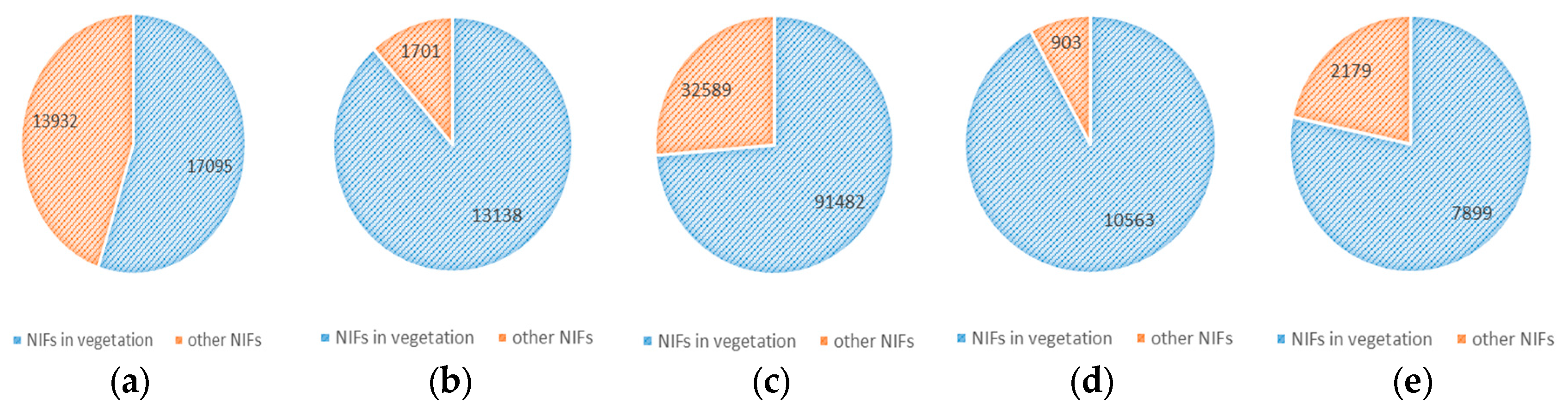
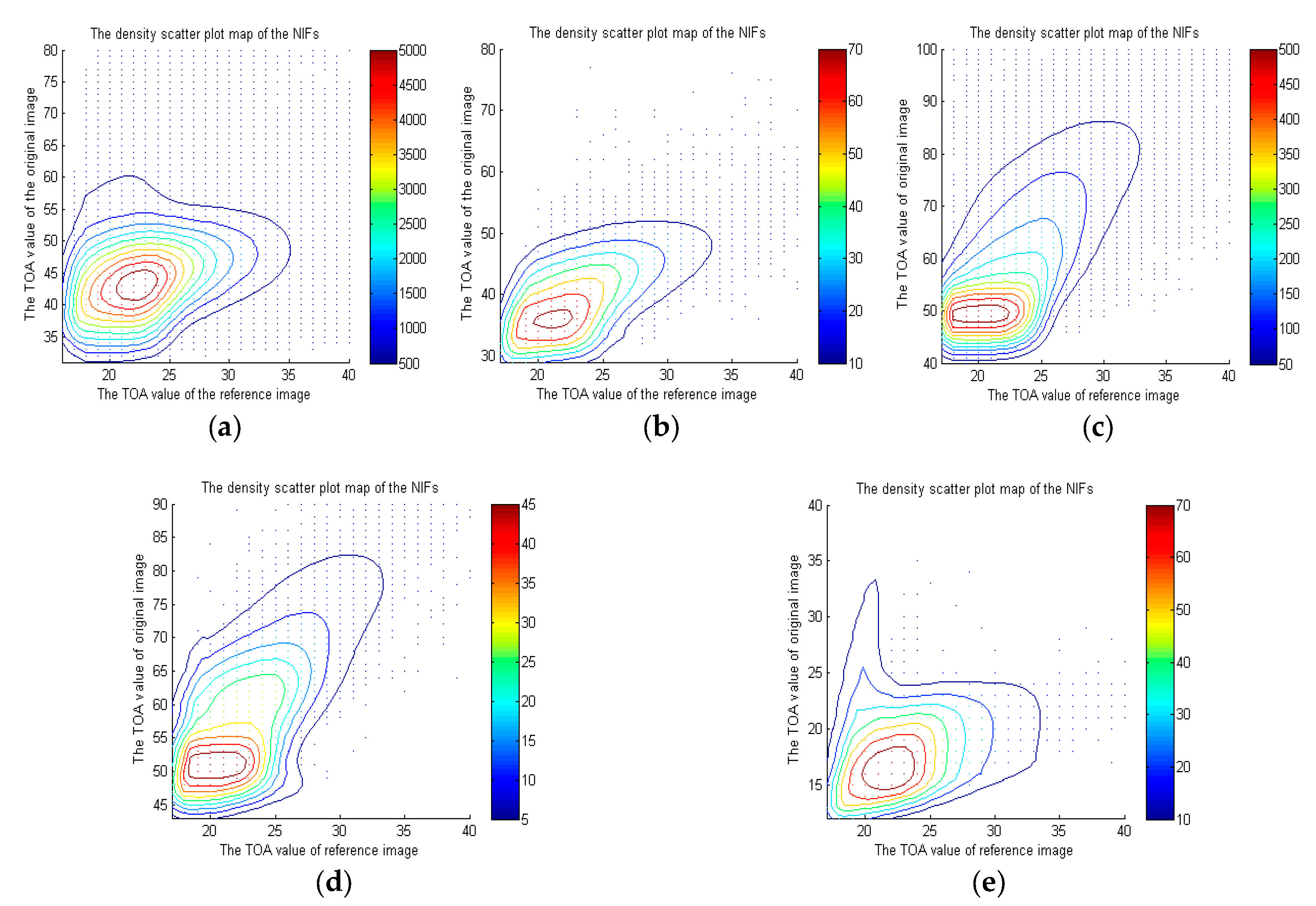
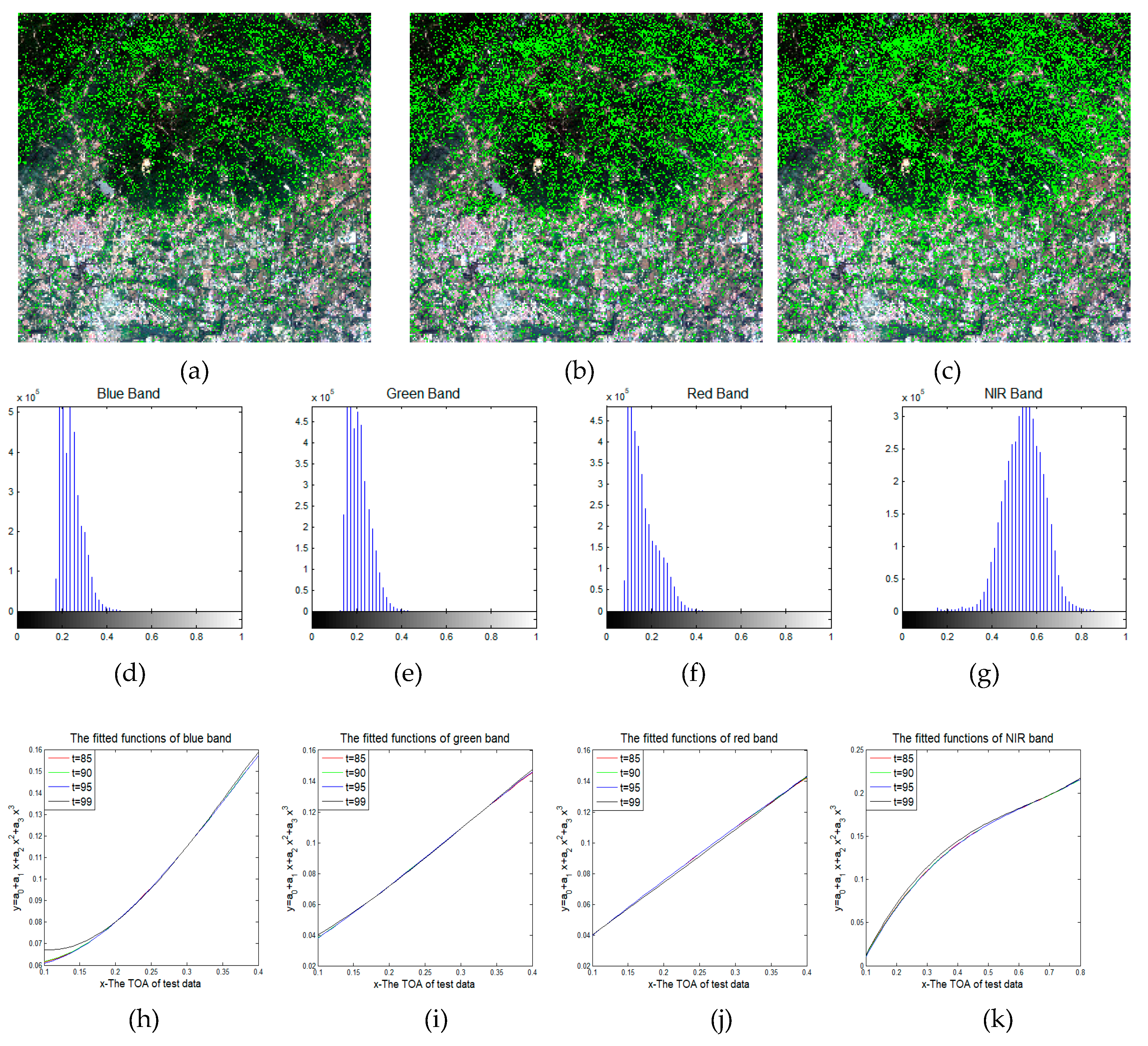
3.2. NIFs Distribution Map

The parameters of the kCCA-based method used to extract NIFs include the regularization parameter ${\epsilon }_1=0.0001$ and threshold of $Pr\left(nochange\right)\mathsf{\tau }=99\%$.

The distribution map of the extracted NIFs is indicated in Figure 3, where the NIFs are represented by green points. The total numbers of NIFs in image 0330, image 0403, image 0705, image 0717 and image 1214 are 31027, 14839, 124071, 11466 and 10078, respectively. Most of NIFs locate in the vegetation area. The proposed method can extract much more NIFs than that of CCA-based method, which only extracts 2432, 2382, 1014, 2074 and 1069 PIFs, respectively. Here the points with a normalized vegetation index (NDVI) larger than 0.2 are considered as vegetation targets. Figure 4 shows the ratio of NIFs in vegetation area to the total number of NIFs. The blue one in pie chart represents the percentage of NIFs in vegetation area. The ratio of NIFs in vegetation area are 55.1%, 88.5%, 83.4%, 92.1% and 78.4%, respectively.

According to the distribution map of NIFs, kCCA can select more NIFs than CCA, which indicates that the spectral variation of the corresponding points between the image-pair are mostly nonlinear. Moreover, since most NIFs are distributed in the vegetation area, it indicates that the spectral changes caused by vegetation growth over time are regular and predictable, and thus they can be detected by NIFs.

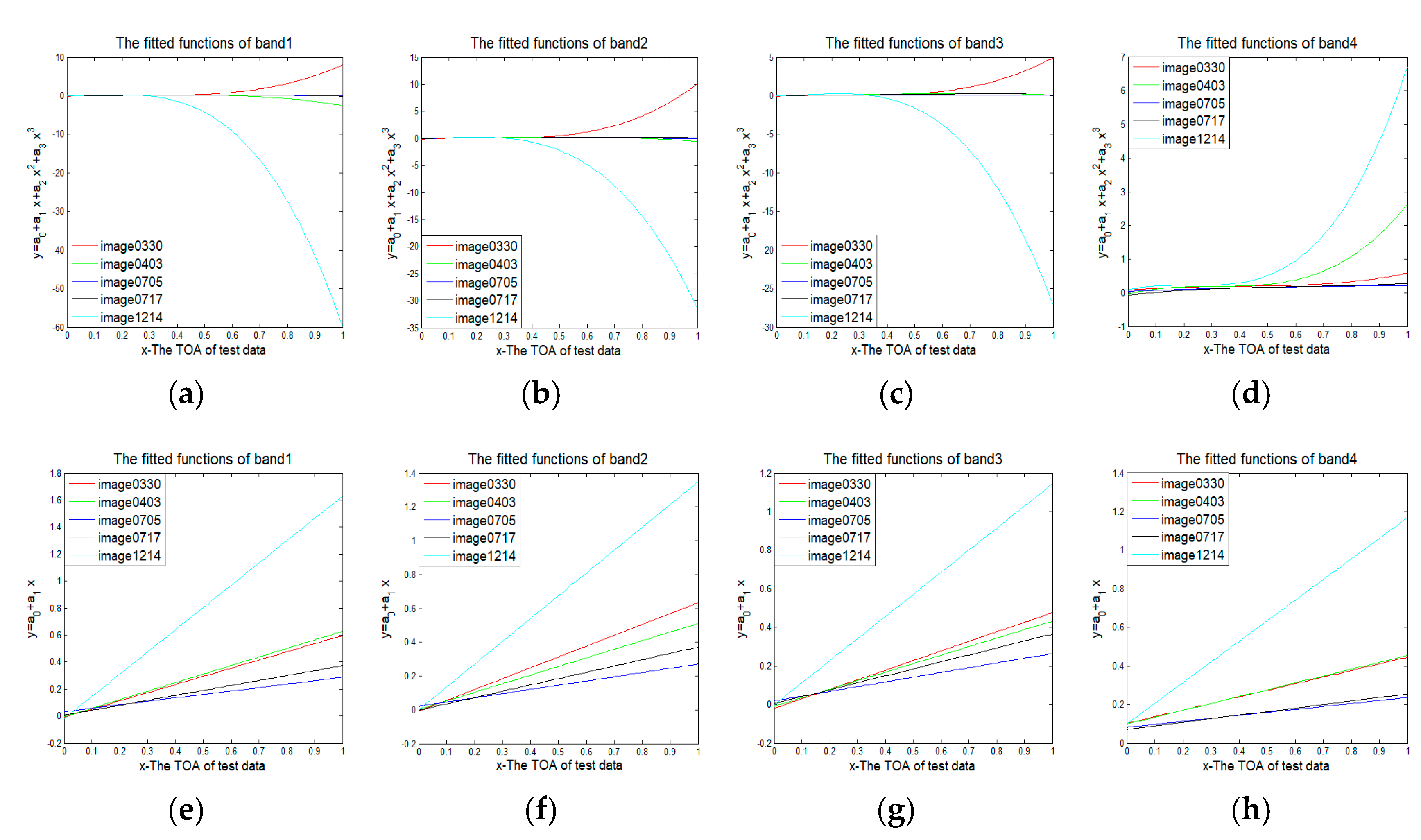
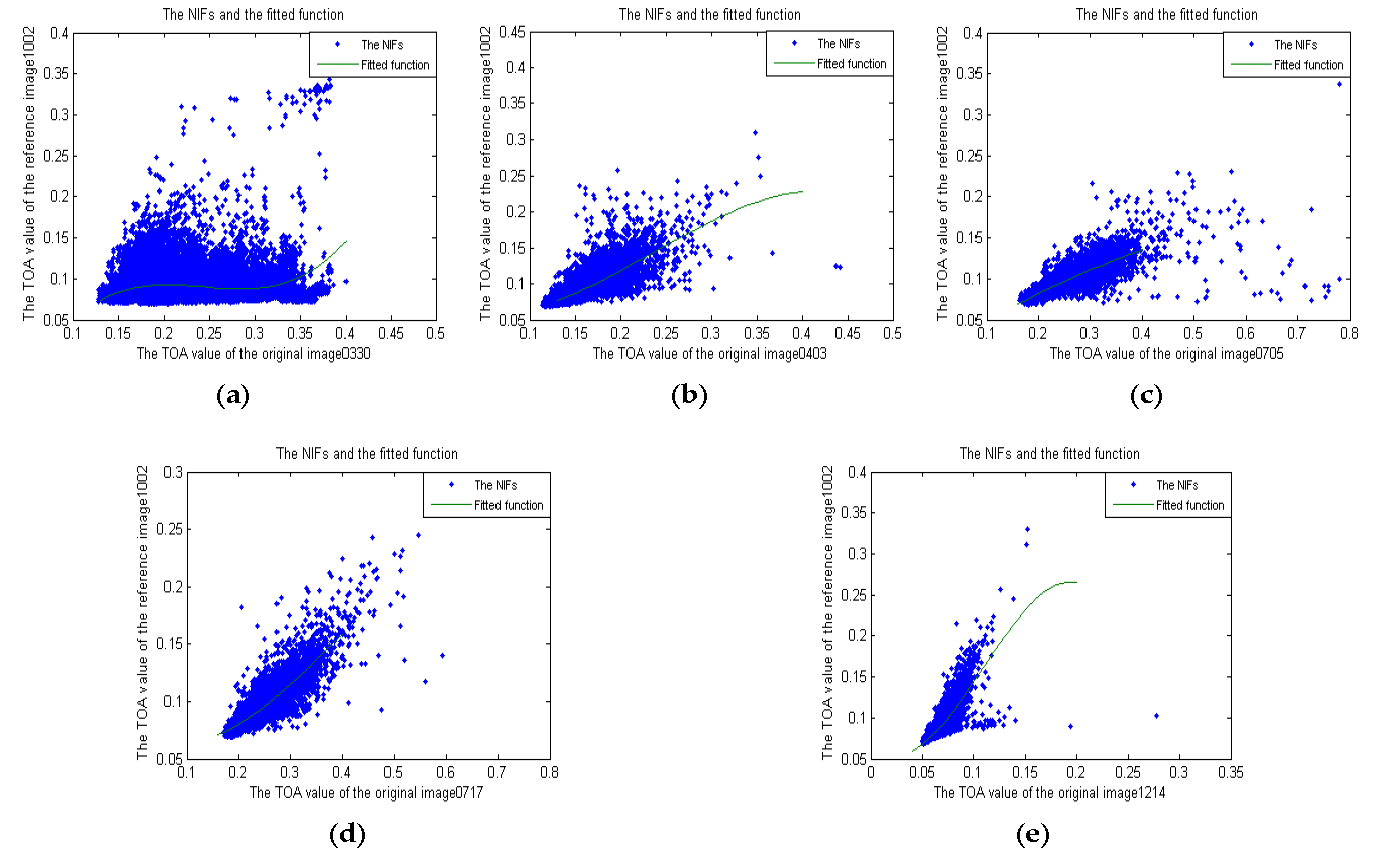
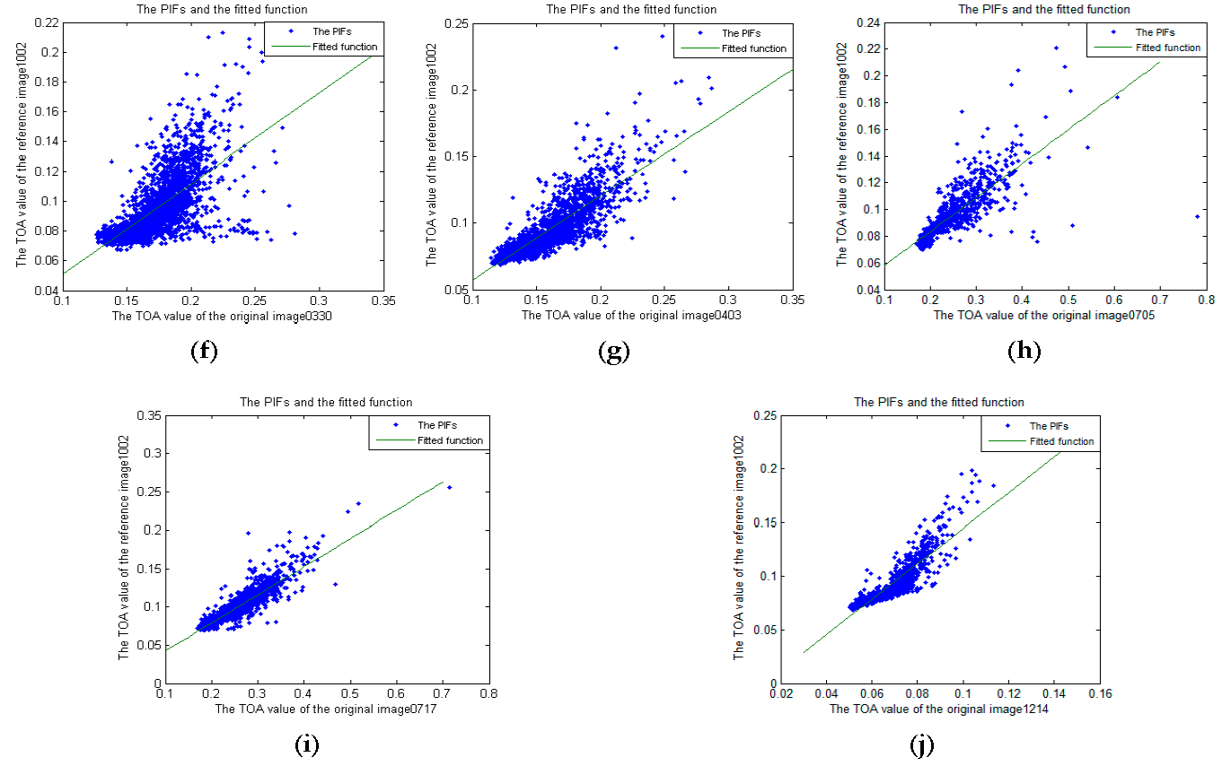
3.3. Derive Nonlinear Transformations from NIFs

Figure 5 is the scatter plot of the density of the NIFs in blue band of test data. The horizontal axis is the TOA value of the test data that linearly stretched from 0–1 to 0–255. The vertical axis is the corresponding value of the reference image. This density map apparently shows the non-linearity of NIFs between image-pairs.

Table 3. The coefficients and error ratios of regression equation a_0, a₁, a₂ and a₃ represent the coefficients of the constant term, the linear term, the quadratic term, and the cubic term, respectively. M_r is the average of the difference between the function value and the expected value, and S_r is the standard deviation.

		a3	a2	a1	a0	Mr	Sr
Image 0330	Band1	18.3284	−13.3953	3.1748	−0.1532	0.019194	0.000002
	Band2	21.5494	−14.4433	3.1393	−0.1489	0.019906	0.000003
	Band 3	10.9105	−7.7441	1.8255	−0.0855	0.02473	0.000004
	Band4	1.4785	−1.7238	0.7561	0.072	0.035371	0.000007
Image 0403	Band1	−7.367	5.2422	−0.5349	0.0748	0.011784	0.000012
	Band2	−3.0287	2.4336	−0.0403	0.0372	0.01312	0.000013
	Band 3	−1.8955	2.0456	−0.099	0.0288	0.018398	0.000015
	Band4	7.3705	−6.866	2.1832	−0.046	0.030512	0.000037
Image 0705	Band1	−0.7959	0.4918	0.194	0.0297	0.010231	0.000024
	Band2	−0.4582	0.0524	0.3273	0.0071	0.011725	0.00002
	Band 3	0.173	−0.4517	0.4073	0.0041	0.015785	0.000023
	Band4	0.0878	−0.2848	0.3699	0.0379	0.0341	0.000083
Image 0717	Band1	−2.2136	2.4316	−0.445	0.0895	0.008238	0.000082
	Band2	−0.7765	0.7466	0.1471	0.0187	0.009817	0.00005
	Band 3	−0.0018	0.0113	0.3381	0.0061	0.013293	0.000033
	Band4	0.6642	−1.2344	0.9188	−0.0681	0.031373	0.000042
Image 1214	Band1	−87.0617	28.3288	−1.1949	0.0675	0.010096	0.000023
	Band2	−44.4402	12.7071	0.2623	0.02687	0.011614	0.000023
	Band 3	−41.5801	14.5948	−0.1363	0.0267	0.017183	0.000032
	Band4	13.8154	−9.1873	2.0127	0.07651	0.026603	0.000044

shows the fitting coefficients and regression error of Equation (27). M_r is the average of the residuals and S_r is the standard deviation of the residuals. As indicated in Table 3, the absolute values of the cubic coefficients of image0330, image0403 and image1214 are significantly larger than those of image0705 and image0717.

Figure 6 shows the transformation function between test image-pair. The red, green, purple, black, and cyan-blue curve denotes the transformation function between the image-pair (image0330, image1002), (image0403, image1002), (image0705, image1002), (image0717, image1002), and (image1214, image1002), respectively. (a–d) are the results fitted by NIFs, (e–h) are results fitted by PIFs. From (a–h), we find that the nonlinear relationship fitted by NIFs between image-pairs increases with the time span. Similarly, the absolute value of the cubic coefficient in Table 3 is relatively larger and the slope of the linear relationship fitted by PIFs also increase with the time span.

Figure 7a–e shows a superimposed display of the NIFs and the fitted curve of NIFs and Figure 7f–j shows that of the PIFs and the curve of the fitted functions based on the PIFs described in Figure 6.

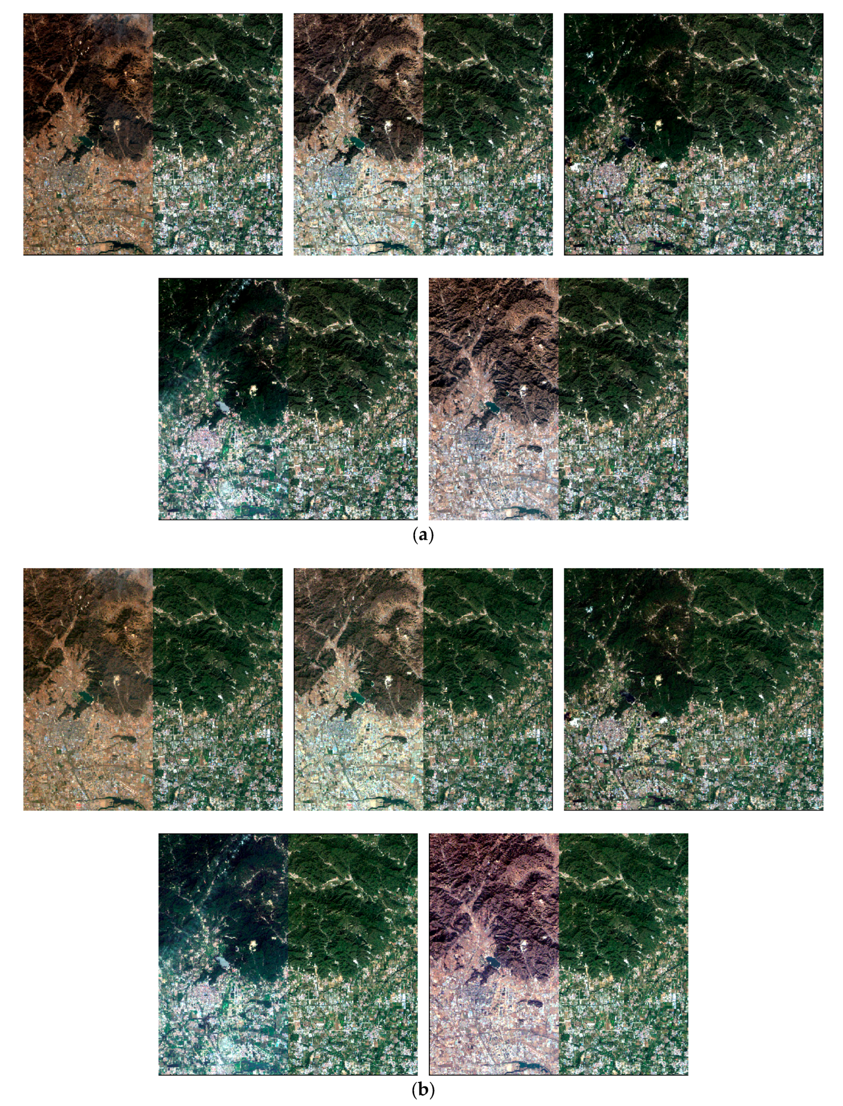
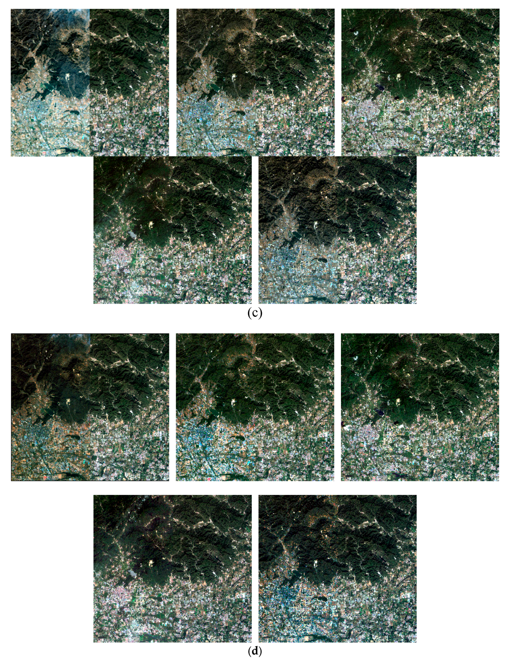
3.4. Radiometric Normalization Results

According to the transformation given in Table 3, the image can be radiometrically normalized. Figure 8 shows the radiation normalization results of the CCA, kCCA and the histogram matching. Each image in Figure 8 is a mosaic image of the reference image (right) and the normalization result (left). Figure 8a shows the original mosaic images and the reference, in which the spectrums of the image-pairs are visually different and in particular, the spectral difference of vegetation increases with the time span between the image-pair. The normalization results of the PIFs-based method (Figure 8b) show that the spectral differences still exist, especially in the vegetation area. The normalization results of the kCCA-based method (Figure 8c) show the spectral differences are significantly reduced, even though the vegetation in spring of image0330 and in winter of image1214 shows similar spectral characteristics with the vegetation in early autumn of image1002. The results of the histogram matching (Figure 8d) show that spectral differences are well reduced.

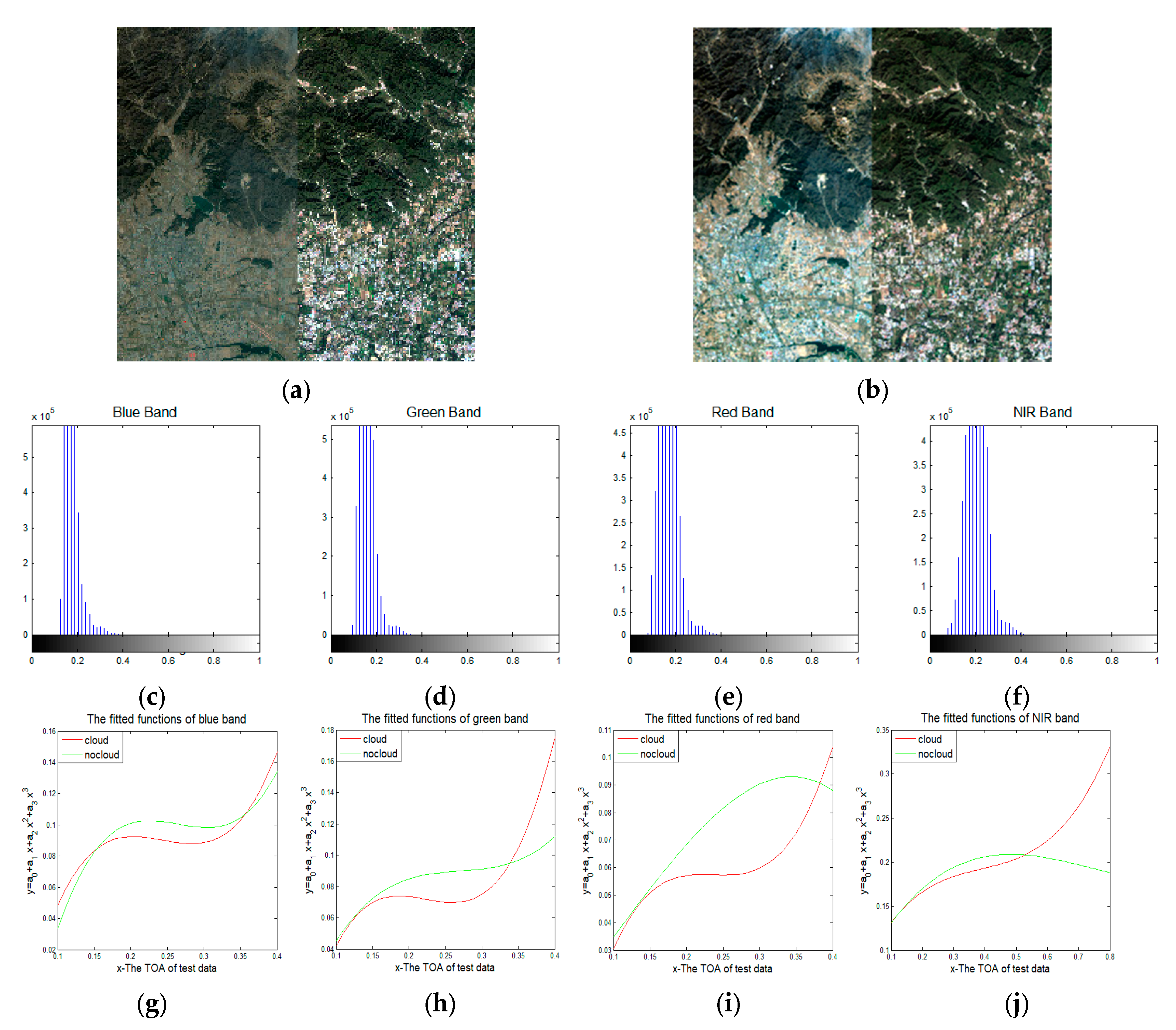
3.4.1. Clouds Pixels in the Image

Towards a quantitative comparison of the proposed radiometric normalization with the CCA-based method and with the histogram matching method, we first discuss the effects of cloud pixels and threshold τ for NIFs extraction and radiometric normalization transformation. The effect caused by cloud pixels is an unavoidable problem that must be considered in remote sensing image radiometric normalization. The usual approach is to mask out the cloud pixels from an image-pair. We use the automatic threshold method to do cloud detection [36]. In fact, if cloud pixels are falsely selected as NIFs, bias will be induced into transformation. The image0330 with clouds is randomly selected as a test image. Following the NIFs extraction steps in Section 3.2, if the cloud pixels have not been masked out, some cloud pixels are selected as NIFs, as shown in the distribution map of NIFs (Figure 3a).

Figure 9a,b show the radiometric normalization results of image0330, showing NIFs with and without cloud pixels. Visually, the brightness of the result including cloud pixels is relatively lower. This can be explained by the normalization transformation derived from NIFs. Figure 9c–f show the histogram of image0330, where we can see that the pixel values are mainly concentrated in [0.1, 0.4]. Figure 9g–j are the fitting curves of the four bands of the image-pair (image0330, image1002). The red and green curves denote the fitted curve from NIFs with and without the cloud pixels, respectively. According to the histogram, we notice that the TOA values of NIFs are mostly distributed between 0.1 and 0.4. In this interval, the fitting values of the NIFs without cloud pixels in Figure 9 are obviously larger than that of the NIFs with cloud pixels, while out of this interval, the fitting values of the NIFs without cloud pixels is smaller. The resulting normalized image of NIFs with cloud fitting is darker than that without cloud fitting.

3.4.2. The Threshold Parameters τ for NIFs Extraction

We use the formula $Pr\left(nochange\right)=1-P_{{\chi }^2,N}\left(Z\right)>\mathsf{\tau }$ to extract the NIFs. The threshold $\mathsf{\tau }$ directly determines the number of NIFs selected. The number of NIFs increases with the value of $\mathsf{\tau }$. In Section 3, $\mathsf{\tau }=0.99$ is used. Here we set the threshold to 0.95, 0.90 and 0.85 respectively to investigate the changes of NIFs distribution map and the normalization function.

Table 4. The number of NIFs with different $\mathsf{\tau }$ .

	$\mathit{\tau }=0.99$	$\mathit{\tau }=0.95$	$\mathit{\tau }=0.90$	$\mathit{\tau }=0.85$
Total number of NIFs	11466	27596	41421	53453
NIFs in vegetation area	10563	25319	38021	49097
Ratio of NIFs in vegetation area (%)	92.12	91.75	91.79	91.85

is the number of NIFs with different τ of the image pair (image0717, image1002). It shows that the total number of NIFs and the number of NIFs in the vegetation area increase as the τ decreases, and the ratio change of NIFs in vegetation area changes is <0.5%, which is relatively stable. Figure 10a–c show the distribution maps of NIFs with different threshold τ. Figure 10d–g show the histogram of image0717. We can see that the pixel values of the red, green, and blue bands are mainly concentrated in [0.1, 0.4], and the pixel values of near infrared band are distributed between 0.1 and 0.8. Figure 10h–k are the fitting curves of the four bands using the above NIFs. It shows that the fitting curves for different thresholds τ are very similar in the corresponding interval range of the TOA values.

3.4.3. Quantitative Comparison of the Radiometric Normalization Results

We use the root mean square error (RMSE), Pearson correlation coefficient and histogram similarity to evaluate the similarity of the radiometric normalization results of proposed method with the CCA-based method and the histogram matching method.

RMSE is used to evaluate the similarity between the normalized image and the reference image. RMSE is defined as follows,

$${\mathrm{RMSE}}_k=\sqrt{\frac{1}{\left|scene\right|}{{\displaystyle \sum }}_{scene}{\left(S_k-R_k\right)}^2},$$

(33)

where $X_i$ is the pixel value of the normalized data, $Y_i$ is the pixel value of the reference image, and $\left|scene\right|$ is the total number of pixels. The smaller the value of RMSE is, the higher the similarity of the two images is.

Pearson correlation coefficient is used to measure the linear correlation between the normalized image and the reference image. The Pearson correlation coefficient is defined as follows,

$$\rho =\frac{{\displaystyle \sum }\left(X_i-\overline{X}\right)\left(Y_i-\overline{Y}\right)}{\sqrt{{\displaystyle \sum }{\left(X_i-\overline{X}\right)}^2}{\displaystyle \sum }{\left(Y_i-\overline{Y}\right)}^2},$$

(34)

where $X_i$ denotes pixel value of the normalized data, $\overline{X}$ denotes the average of the normalized data, $Y_i$ denotes the corresponding pixel value of the reference data, and $\overline{Y}$ denotes the average of the reference data.

Histogram similarity measured by the histogram correlation which is used to calculate the linear correlation between the two histograms of the normalized image and the reference image. The histogram correlation is defined as follows,

$$\rho \left(H1,H2\right)=\frac{{\displaystyle \sum }\left(H{1}_i-\overline{H1}\right)\left(H{2}_i-H2\right)}{\sqrt{{\displaystyle \sum }{\left(H{1}_i-\overline{H1}\right)}^2}{\displaystyle \sum }{\left(H{2}_i-\overline{H2}\right)}^2},$$

(35)

where $H1$ is the histogram of the normalized data, $\overline{H1}$ is the mean of $H1$, $H2$ is the histogram of the reference data, $\overline{H2}$ is the mean of $H2$. The similarity positively correlates to the histogram correlation.

Table 5. RMSE is the RMSE of the test data and reference image, $\mathsf{\rho }$ is the Pearson correlation coefficients of the test data and reference image, ${\mathsf{\rho }}_h$ is histogram correlation of the test data and reference image.

	RMSE	$\mathsf{\rho }$	${\mathsf{\rho }}_{\mathit{h}}$
image pair (imag0330, image1002)
Band 1	0.09	0.32	0.04
Band 2	0.09	0.40	0.03
Band 3	0.12	0.45	-0.05
Band 4	0.06	0.36	0.74
image pair (imag0403, image1002)
Band 1	0.07	0.80	0.02
Band 2	0.07	0.77	0.05
Band 3	0.10	0.71	-0.02
Band 4	0.06	0.51	0.69
image pair (imag0705, image1002)
Band 1	0.15	0.80	0.07
Band 2	0.15	0.77	0.09
Band 3	0.13	0.78	0.09
Band 4	0.42	0.40	0.24
image pair (imag0717, image1002)
Band 1	0.15	0.89	0.07
Band 2	0.14	0.87	0.08
Band 3	0.11	0.86	0.07
Band 4	0.38	0.46	0.23
image pair (imag1214, image1002)
Band 1	0.03	0.81	0.43
Band 2	0.02	0.81	0.78
Band 3	0.02	0.73	0.75
Band 4	0.11	0.67	-0.04

and

Table 6. RMSE^CCA is the RMSE of the radiometric normalization results based on CCA algorithm, RMSE^kCCA is the RMSE of the results based on NIFs extracted by the kCCA transformation, RMSE^H is the RMSE of the results based on the histogram matching method. $\mathsf{\rho }$^CCA, $\mathsf{\rho }$^kCCA and $\mathsf{\rho }$^H are the Pearson correlation coefficients of the radiometric normalization results based on the CCA algorithm, kCCA transformation and the histogram matching method. ${\mathsf{\rho }}_h^{CCA}$, ${\mathsf{\rho }}_h^{kCCA}$ and ${\mathsf{\rho }}_h^H$ are histogram correlation of the radiometric normalization results based on the CCA algorithm, kCCA transformation and the histogram matching method.

	RMSECCA	RMSEkCCA	RMSEH	$\mathsf{\rho }$CCA	$\mathsf{\rho }$kCCA	$\mathsf{\rho }$H	${\mathsf{\rho }}_{\mathit{h}}^{\mathit{C}\mathit{C}\mathit{A}}$	${\mathsf{\rho }}_{\mathit{h}}^{\mathit{k}\mathit{C}\mathit{C}\mathit{A}}$	${\mathsf{\rho }}_{\mathit{h}}^{\mathit{H}}$
image pair (imag0330, image1002)
Band 1	0.02	0.02	0.02	0.32	0.42	0.32	0.58	0.69	0.98
Band 2	0.02	0.02	0.02	0.40	0.47	0.39	0.77	0.78	0.97
Band 3	0.03	0.02	0.03	0.45	0.47	0.41	0.73	0.75	0.98
Band 4	0.04	0.03	0.04	0.36	0.37	0.37	0.81	0.82	0.94
image pair (imag0403 image1002)
Band 1	0.01	0.01	0.01	0.81	0.81	0.80	0.95	0.95	0.98
Band 2	0.01	0.01	0.01	0.78	0.78	0.77	0.93	0.93	0.99
Band 3	0.02	0.02	0.02	0.71	0.72	0.71	0.86	0.93	0.99
Band 4	0.06	0.03	0.04	0.51	0.55	0.55	0.74	0.89	0.95
image pair (imag0705, image1002):
Band 1	0.02	0.01	0.01	0.80	0.83	0.81	0.92	0.93	1.00
Band 2	0.02	0.01	0.01	0.77	0.80	0.78	0.98	0.94	0.91
Band 3	0.03	0.01	0.02	0.78	0.79	0.77	0.97	0.91	0.88
Band 4	0.06	0.03	0.04	0.41	0.42	0.38	0.82	0.81	0.99
image pair (imag0717, image1002):
Band 1	0.01	0.01	0.01	0.89	0.89	0.89	0.94	0.94	0.99
Band 2	0.01	0.01	0.01	0.87	0.87	0.87	0.94	0.94	0.98
Band 3	0.02	0.01	0.01	0.86	0.86	0.86	0.93	0.93	0.98
Band 4	0.06	0.03	0.04	0.47	0.47	0.46	0.88	0.88	0.99
image pair (imag1214, image1002):
Band 1	0.01	0.01	0.01	0.83	0.85	0.85	0.81	0.85	0.85
Band 2	0.01	0.01	0.01	0.81	0.82	0.82	0.86	0.88	0.88
Band 3	0.02	0.02	0.02	0.74	0.76	0.74	0.74	0.79	0.86
Band 4	0.03	0.03	0.03	0.67	0.68	0.67	0.77	0.90	0.92

are the RMSE, Pearson correlation coefficient and histogram similarity between each multi-temporal image and the reference image before and after radiometric normalization. Here RMSE^CCA is RMSE of the radiometric normalization results from the CCA-based method, RMSE^kCCA is RMSE of the results from the kCCA-based transformation, and RMSE^H is RMSE of the results from the histogram matching method. ${\mathsf{\rho }}^{CCA}$, ${\mathsf{\rho }}^{kCCA}$ and ${\mathsf{\rho }}^H$ are Pearson correlation coefficients of the radiometric normalization results from the CCA-based, kCCA-based and the histogram matching methods, respectively. ${\mathsf{\rho }}_h^{CCA}$, ${\mathsf{\rho }}_h^{kCCA}$ and ${\mathsf{\rho }}_h^H$ are histogram correlation of the radiometric normalization results from the CCA-based, kCCA-based and the histogram matching methods, respectively.

4. Discussion

The paper focused on the radiometric normalization of satellite image sequence analysis, especially, the elimination of the spectral difference among the images caused by different image acquisition conditions and the effects of the regularly nonlinear spectral differences caused by seasonal variation of natural objects. We proposed a novel method, i.e., the kCCA, to select nonlinear radiation control points-NIFs and to derive the nonlinear transformation of image-pairs using the least squares regression method.

The total number of the selected NIFs were larger than that of the linear radiometric normalization method (CCA). This indicates that the spectral variation of the corresponding points between each image-pair is mostly nonlinear. Moreover, since most NIFs were distributed in the vegetation area, it indicates that the spectral changes caused by vegetation growth over time are regular and predictable, and thus they can be detected by NIFs. Figure 9 showed us that the effect of cloud pixels was a problem that must be considered in the extraction of NIFs and that the removal of cloud pixels can improve the accuracy of radiometric normalization. The chi-squared percentile τ directly determined the number of NIFs. Table 4 showed that the total number of NIFs and the number of NIFs in the vegetation area increased as the τ decreased. However, the ratio of NIFs in vegetation area was relatively stable and the fitting curves for different thresholds τ were similar. Therefore, we should appropriately choose the value of τ so that we can get enough invariant points to fit the nonlinear relationship. If the value of τ is too small, the numbers of NIFs will be quite large, which leads to higher computation afford.

By using of the least squares regression, we have derived relationships between image-pairs from NIFs. The scatter plot map of the NIFs density (Figure 5) showed us that the relationships were nonlinear. Table 3 and Figure 6 showed that the nonlinear relationship positively correlated with the time span between image-pairs.

Table 5 and Table 6 showed that the kCCA-based nonlinear radiometric normalized images had the smallest RMSE and the largest correlation coefficient with the reference image. As the time span increased, the RMSE increased and the correlation coefficient decreased, and so was that of the normalized images based on the CCA method. Radiometric normalized images of the histogram matching method had the largest RMSE and the smallest correlation coefficient with the reference image. It means the kCCA-based normalization can preserve more similarity and better correlation between image-pairs than the CCA algorithm and histogram matching. Histogram similarity is an index that measures the color difference between an image-pair. The histograms of the radiometric normalized images using the histogram matching had the highest histogram similarity with the reference image, those of kCCA transformation had the second highest similarity, while the CCA-based linear radiometric normalized results had the lowest similarity. However, the histogram matching uses global statistical information for normalization which eliminates all the spectral difference between an image-pair, including the difference must be preserved. Compared with the CCA-based linear normalization, the proposed method can better avoid the color error propagation.

In general, the kCCA-based normalization can either preserve more similarity and correlation between each image-pair or effectively avoid the color error propagation. The proposed method not only builds the common scale or reference to make the radiometric consistency among GF-1 image sequences, but also highlights the interesting spectral changes while eliminates less interesting spectral changes. Our method enables the application of GF-1 data for change detection, land-use, land-cover change detection etc.

5. Conclusions

In this paper, we presented a novel method to perform nonlinear relative spectral alignment and radiometric normalization for high-resolution wide-spectrum multi-temporal satellite images. The method used the kernel canonical correlation analysis transformation (kCCA) to extract NIFs, a set of samples belonging to unchanged area in the kernel space, and to align the relative spectrum of two images using the NIFs-fitted nonlinear relationship. The proposed approach does not need full supervision. The presented approach may be used as a preprocessing technique for change detection of multi-temporal images, especially when the vegetation spectral changes of multi-temporal images is a disturbance of change detection. Furthermore, we qualitatively and quantitatively compared the radiometric normalization results of the proposed method with CCA-based PIFs method and the histogram matching method derived from statistical distribution. The comparison indicated that the radiometric normalization result of the proposed method had the best linear correlation and least bias with the reference, whereas the radiometric normalization of the histogram matching had the best histogram similarity with the reference image. Finally, in this paper we dealt only with pixel-wise approaches for both the relative spectral alignment and radiometric normalization using the polynomial kernel canonical correlation analysis transformation. In future, we will address the use of different kernel function space, mixed kernel function space and the spatial context to improve both the alignment and the radiometric normalization. This would open many applications of very high-resolution imagery, because high-resolution multi-temporal image-pairs have more complex non-linear relationship and the semantic classes cannot be modeled pixel-wise.

References

1. Bai, Y.; Tang, P.; Hu, C.M. Kernel Mad Algorithm for Relative Radiometric Normalization. Int. Arch. Photogramm. 2016, 3, 49–53. [Google Scholar] [CrossRef]
2. Song, C.; Woodcock, C.E.; Seto, K.C.; Lenney, M.P.; Macomber, S.A. Classification and change detection using Landsat TM data: When and how to correct atmospheric effects? Remote Sens. Environ. 2001, 75, 230–244. [Google Scholar] [CrossRef]
3. Yang, Q.-H.; Qi, J.-W.; Sun, Y. The application of high-resolution satellite remotely sensed data to landuse dynamic monitoring. Remote Sens. Land Resour. 2002, 4, 20–27. [Google Scholar]
4. Yang, X.J.; Lo, C.P. Relative radiometric normalization performance for change detection from multi-date satellite images. Photogramm. Eng. Remote Sens. 2000, 66, 967–980. [Google Scholar]
5. Barazzetti, L.; Gianinetto, M.; Scaioni, M. Radiometric Normalization with Multi-image Pseudo-invariant Features. In Proceedings of the Fourth International Conference on Remote Sensing and Geoinformation of the Environment (Rscy2016), Paphos, Cyprus, 4–8 April 2016. [Google Scholar]
6. Hu, C.M.; Tang, P. Automatic algorithm for relative radiometric normalization of data obtained from Landsat TM and HJ-1A/B charge-coupled device sensors. J. Appl. Remote Sens. 2012, 6. [Google Scholar] [CrossRef]
7. Volpi, M.; Camps-Valls, G.; Tuia, D. Spectral alignment of multi-temporal cross-sensor images with automated kernel canonical correlation analysis. J. Photogramm. Remote Sens. 2015, 107, 50–63. [Google Scholar] [CrossRef]
8. Berk, A.; Anderson, G.P. Impact of MODTRAN®5.1 on atmospheric compensation. In Proceedings of the 2008 IEEE International Geoscience and Remote Sensing Symposium, Boston, MA, USA, 6–11 July 2008; pp. 127–129. [Google Scholar]
9. El Hajj, M.; Begue, A.; Lafrance, B.; Hagolle, O.; Dedieu, G.; Rumeau, M. Relative radiometric normalization and atmospheric correction of a SPOT 5 time series. Sensors 2008, 8, 2774–2791. [Google Scholar] [CrossRef] [PubMed]
10. Philpot, W.; Ansty, T. Analytical Description of Pseudoinvariant Features. IEEE Trans. Geosci. Remote Sens. 2013, 51, 2016–2021. [Google Scholar] [CrossRef]
11. Canty, M.J.; Nielsen, A.A.; Schmidt, M. Automatic radiometric normalization of multitemporal satellite imagery. Remote Sens. Environ. 2004, 91, 441–451. [Google Scholar] [CrossRef] [Green Version]
12. De Carvalh, O.A.; Guimaraes, R.F.; Silva, N.C.; Gillespie, A.R.; Gomes, R.A.T.; Silva, C.R.; de Carvalho, A.P.F. Radiometric Normalization of Temporal Images Combining Automatic Detection of Pseudo-Invariant Features from the Distance and Similarity Spectral Measures, Density Scatterplot Analysis, and Robust Regression. Remote Sens. 2013, 5, 2763–2794. [Google Scholar] [CrossRef]
13. Schott, J.R.; Salvaggio, C.; Volchok, W.J. Radiometric Scene Normalization Using Pseudo-invariant Features. Remote Sens. Environ. 1988, 6, 1–16. [Google Scholar] [CrossRef]
14. Andrefouet, S.; Muller-Karger, F.E.; Hochberg, E.J.; Hu, C.M.; Carder, K.L. Change detection in shallow coral reef environments using Landsat 7 ETM+ data. Remote Sens. Environ. 2001, 78, 150–162. [Google Scholar] [CrossRef]
15. Chen, X.X.; Vierling, L.; Deering, D. A simple and effective radiometric correction method to improve landscape change detection across sensors and across time. Remote Sens. Environ. 2005, 98, 63–79. [Google Scholar] [CrossRef]
16. Kennedy, R.E.; Cohen, W.B. Automated designation of tie-points for image-to-image coregistration. Int. J. Remote Sens. 2003, 24, 3467–3490. [Google Scholar] [CrossRef]
17. Hall, F.G.; Strebel, D.E.; Nickeson, J.E.; Goetz, S.J. Radiometric Rectification—Toward a Common Radiometric Response among Multidate, Multisensor Images. Remote Sens. Environ. 1991, 35, 11–27. [Google Scholar] [CrossRef]
18. Elvidge, C.D.; Yuan, D.; Weerackoon, R.D.; Lunetta, R.S. Relative Radiometric Normalization of Landsat Multispectral Scanner (Mss) Data Using an Automatic Scattergram-Controlled Regression. Photogramm. Eng. Remote Sens. 1995, 61, 1255–1260. [Google Scholar]
19. Yu, X.; Chen, Y. Relative radiometric normalization of remotely sensed images based on improved automatic scattergram-controlled regression. Opt. Tech. 2007, 22, 185–188. [Google Scholar]
20. Canty, M.J.; Nielsen, A.A. Unsupervised classification of changes in multispectral satellite imagery. Proc. SPIE 2004, 5573, 356–363. [Google Scholar] [CrossRef]
21. Canty, M.J.; Nielsen, A.A. Automatic radiometric normalization of multitemporal satellite imagery with the iteratively re-weighted MAD transformation. Remote Sens. Environ. 2008, 112, 1025–1036. [Google Scholar] [CrossRef]
22. Nielsen, A.A. Multiset canonical correlations analysis and multispectral, truly multitemporal remote sensing data. IEEE Trans. Image Process. 2002, 11, 293–305. [Google Scholar] [CrossRef] [PubMed] [Green Version]
23. Nielsen, A.A.; Conradsen, K.; Simpson, J.J. Multivariate alteration detection (MAD) and MAF postprocessing in multispectral, bitemporal image data: New approaches to change detection studies. Remote Sens. Environ. 1998, 64, 1–19. [Google Scholar] [CrossRef]
24. Sadeghi, V.; Ebadi, H.; Ahmadi, F.F. A new model for automatic normalization of multitemporal satellite images using Artificial Neural Network and mathematical methods. Appl. Math. Model. 2013, 37, 6437–6445. [Google Scholar] [CrossRef]
25. Helmer, E.H.; Ruefenacht, B. A comparison of radiometric normalization methods when filling cloud gaps in Landsat imagery. Can. J. Remote Sens. 2007, 33, 457–458. [Google Scholar] [CrossRef]
26. Canty, M.J.; Nielsen, A.A. Linear and kernel methods for multivariate change detection. Comput. Geosci. 2012, 38, 107–114. [Google Scholar] [CrossRef]
27. Huang, S.Y.; Lee, M.H.; Hsiao, C.K. Nonlinear measures of association with kernel canonical correlation analysis and applications. J. Stat. Plan. Inference 2009, 139, 2162–2174. [Google Scholar] [CrossRef]
28. Nielsen, A.A. Kernel Methods in Orthogonalization of Multi- and Hypervariate Data. In Proceedings of the 2009 16th IEEE International Conference on Image Processing (ICIP), Cairo, Egypt, 7–10 November 2009; pp. 3729–3732. [Google Scholar]
29. Nielsen, A.A.; Vestergaard, J.S. A Kernel Version of Multivariate Alteration Detection. In Proceedings of the 2013 IEEE International Geoscience and Remote Sensing Symposium (IGARSS), Melbourne, VIC, Australia, 21–26 July 2013; pp. 3451–3454. [Google Scholar]
30. Yoshida, K.; Yoshimoto, J.; Doya, K. Sparse kernel canonical correlation analysis for discovery of nonlinear interactions in high-dimensional data. BMC Bioinform. 2017, 18. [Google Scholar] [CrossRef] [PubMed]
31. Shao, J.; Wang, L.Q.; Zhao, Z.C.; Su, F.; Cai, A.N. Deep canonical correlation analysis with progressive and hypergraph learning for cross-modal retrieval. Neurocomputing 2016, 214, 618–628. [Google Scholar] [CrossRef]
32. Hotelling, H. Relations between two sets of variates. Biometrika 1936, 28, 321–377. [Google Scholar] [CrossRef]
33. Camps-Valls, G.; Bruzzone, L. Kernel Methods for Remote Sensing Data Analysis; Wiley: Hoboken, NJ, USA, 2009. [Google Scholar]
34. Shawe-Taylor, J.; Cristianini, N. Kernel Methods for Pattern Analysis; Cambridge University Press: Cambridge, UK, 2004. [Google Scholar]
35. Nielsen, A.A.; Conradsen, K.; Andersen, O. A change oriented extension of EOF analysis applied to the 1996–1997 AVHRR sea surface temperature data. Phys. Chem. Earth 2002, 27, 1379–1386. [Google Scholar] [CrossRef]
36. Hu, C.M.; Bai, Y.; Tang, P. Automatic cloud detection for GF-4 series images. J. Remote Sens. 2018, 22, 132–142. [Google Scholar]
Figure 1. The workflow of kernel CCA.
Remotesensing 10 00432 g001
Figure 2. The GF-1 images of the test area (Beijing, China). The GF-1 data, (af) are image0330, image 0403, image0705, image0717, image1002 and image1214, acquired in 30 March, 3 April, 5 July, 17 July, 2 October, 14 December 2013.
Remotesensing 10 00432 g002
Figure 3. The distribution map of NIFs selected by the kCCA transformation. (ae) are, in order, image0330, image0403, image0705, image0717 and image1214. The green points are the NIFs of each image.
Remotesensing 10 00432 g003
Figure 4. The ratio of NIFs in vegetation area to the total number of NIFs. (ae) refer to the result of image0330, image0403, image0705, image0717 and image1214, respectively. The blue represents the NIFs in vegetation area and the yellow is the other NIFs.
Remotesensing 10 00432 g004
Figure 5. The density scatter plot map of the NIFs. The horizontal axis in the figure is the TOA value of the original image that linearly stretched from 0–1 to 0–255, and the vertical axis is that of the reference image. (ae) refer to the result of image0330, image0403, image0705, image0717 and image1214, respectively.
Remotesensing 10 00432 g005
Figure 6. The fitted functions of the four band for the 5 test GF-1 image-pairs. (ad) refer to the results of band1, band2, Band 3 and band4 based on the proposed method. (eh) are the linear regression equations of the PIFs-based method. —is the fitted function of image0330 and the reference, —is that of image0403 and the reference, —is that of image0705 and the reference, —is that of image0717 and the reference, —is that of image1214 and the reference.
Remotesensing 10 00432 g006
Figure 7. The superimposed display of the NIFs and PIFs distribution map and the curve of the fitted functions based on the NIFs and PIFs described above. The horizontal axis in the figure is the TOA value of the original image, and the vertical axis is that of the reference image. (ae) refer to the NIFs results of image0330, image0403, image0705, image0717 and image1214, respectively. (fj) are that of PIFs results.
Remotesensing 10 00432 g007aRemotesensing 10 00432 g007b
Figure 8. The comparison of the results of radiometric normalization based on the kCCA transformation, the CCA method and the histogram matching. Each image is a mosaic image. The left one is the corrected image, and the right one is the reference image. (a) is the test data and the reference image; (b) is the results of the CCA algorithm and the reference images; (c) is the results based on NIFs extracted by the kCCA transformation; (d) is the results of the histogram matching.
Remotesensing 10 00432 g008aRemotesensing 10 00432 g008b
Figure 9. The results of the radiometric normalization of image0330 based on two NIFs set and the fitted curve of the two normalized results. (a) is the result based on all NIFs (including the cloud-NIFs), (b) is the result based on NIFs without cloud pixels, (cf) are histogram of image0330. (gj) are the fitted curve of four bands of image-pair (image0330 and image1002). — denotes the fitted curve using all NIFs including cloud pixels. — is the fitted curve using NIFs without the cloud pixels.
Remotesensing 10 00432 g009
Figure 10. The distribution map of NIFs based on different threshold τ. The data is image0717. (ac) are the distribution maps when τ = 0.95, τ = 0.90 and τ = 085. (dg) are histogram of four bands of image0717. (hk) are fitting curves of four bands based on the above NIFs.
Remotesensing 10 00432 g010