Matching of Remote Sensing Images with Complex Background Variations via Siamese Convolutional Neural Network


Abstract
1. Introduction
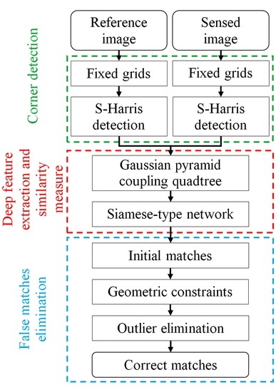
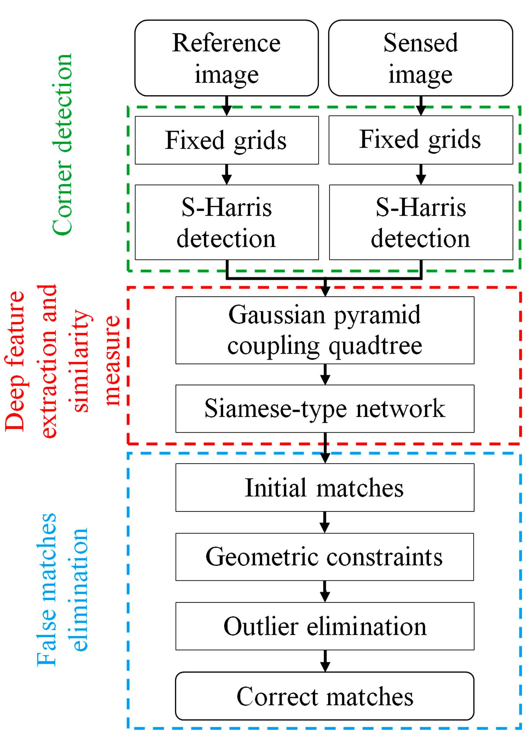
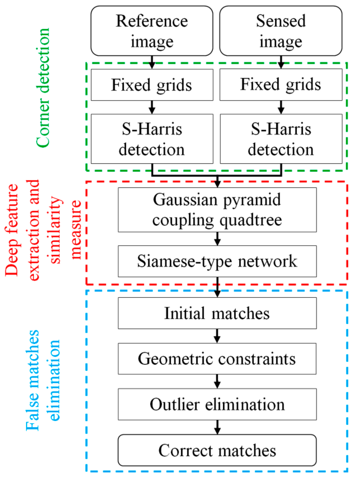
2. Methodology
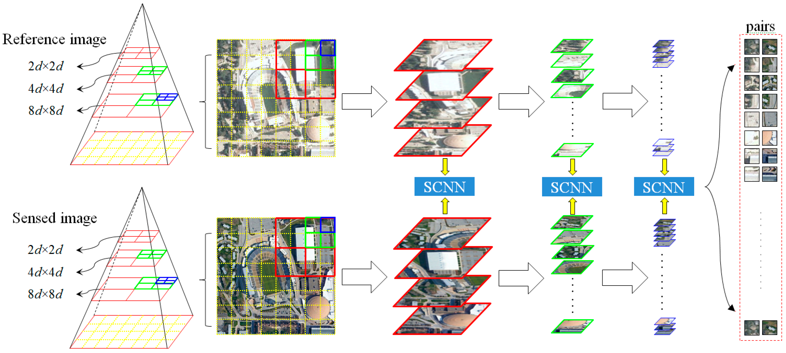
2.1. Siamese Convolutional Neural Network
2.2. Coarse-Conjugated Patch Decision
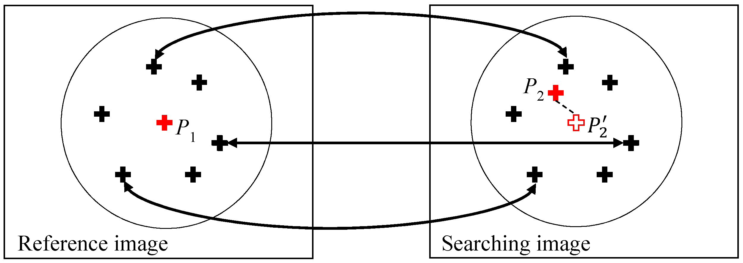
2.3. Multiscale-Conjugated Point Decision
| Algorithm: |
| Input: and are the coarse-conjugated patches in the sensed and reference images, respectively; are the Harris corners in and , and is the number of Harris corners Parameters: matching probability , non-matching probability , and similarity index . Compute the distance of center to Harris corners and in the patches. Traverse the Harris corners based on from min to max. for to do for to do Compute if then Update end for end for Record the coordinates of Harris corners with . |
2.4. Outlier Elimination
3. Experimental Evaluation and Discussion
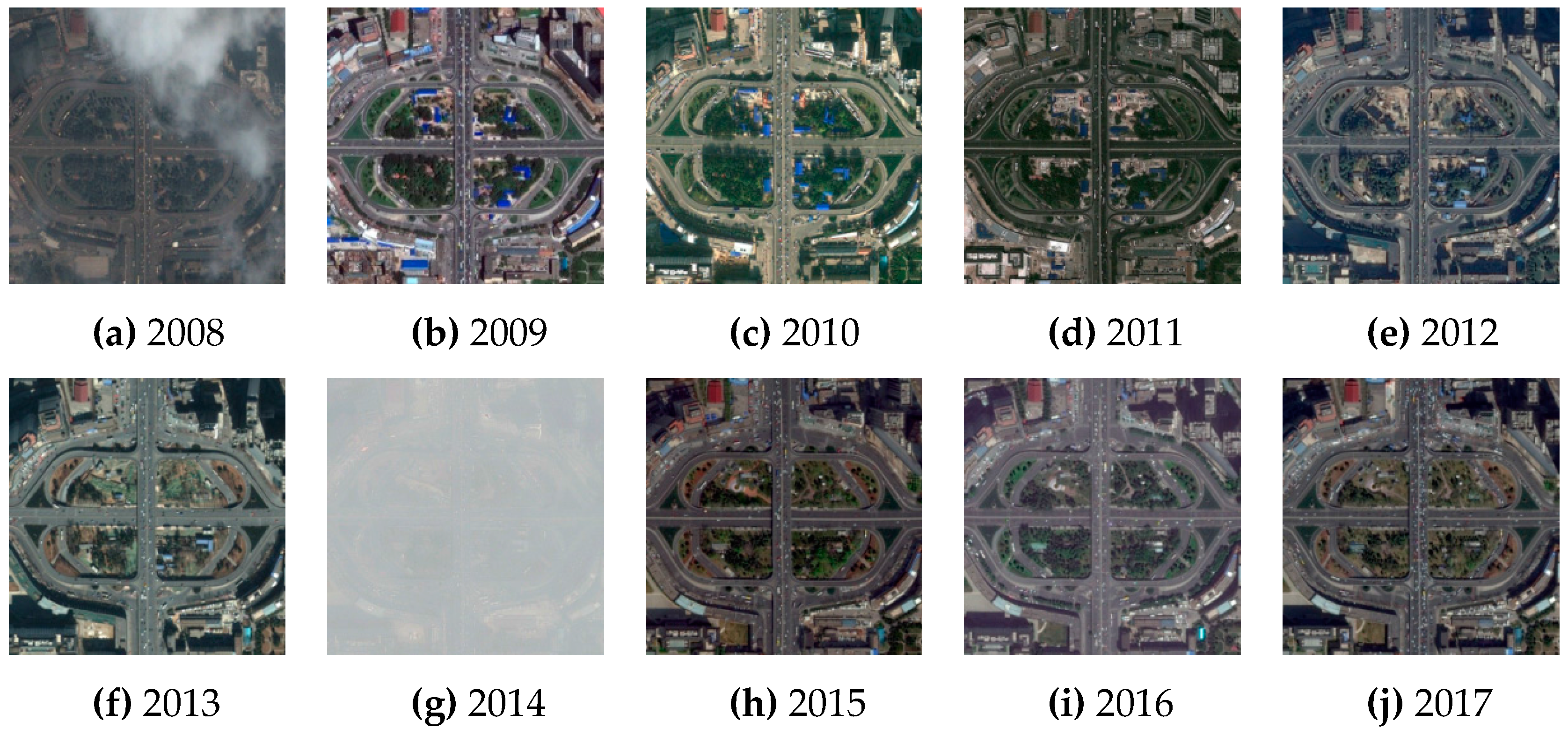
3.1. Experimental Datasets
3.2. SCNN Training
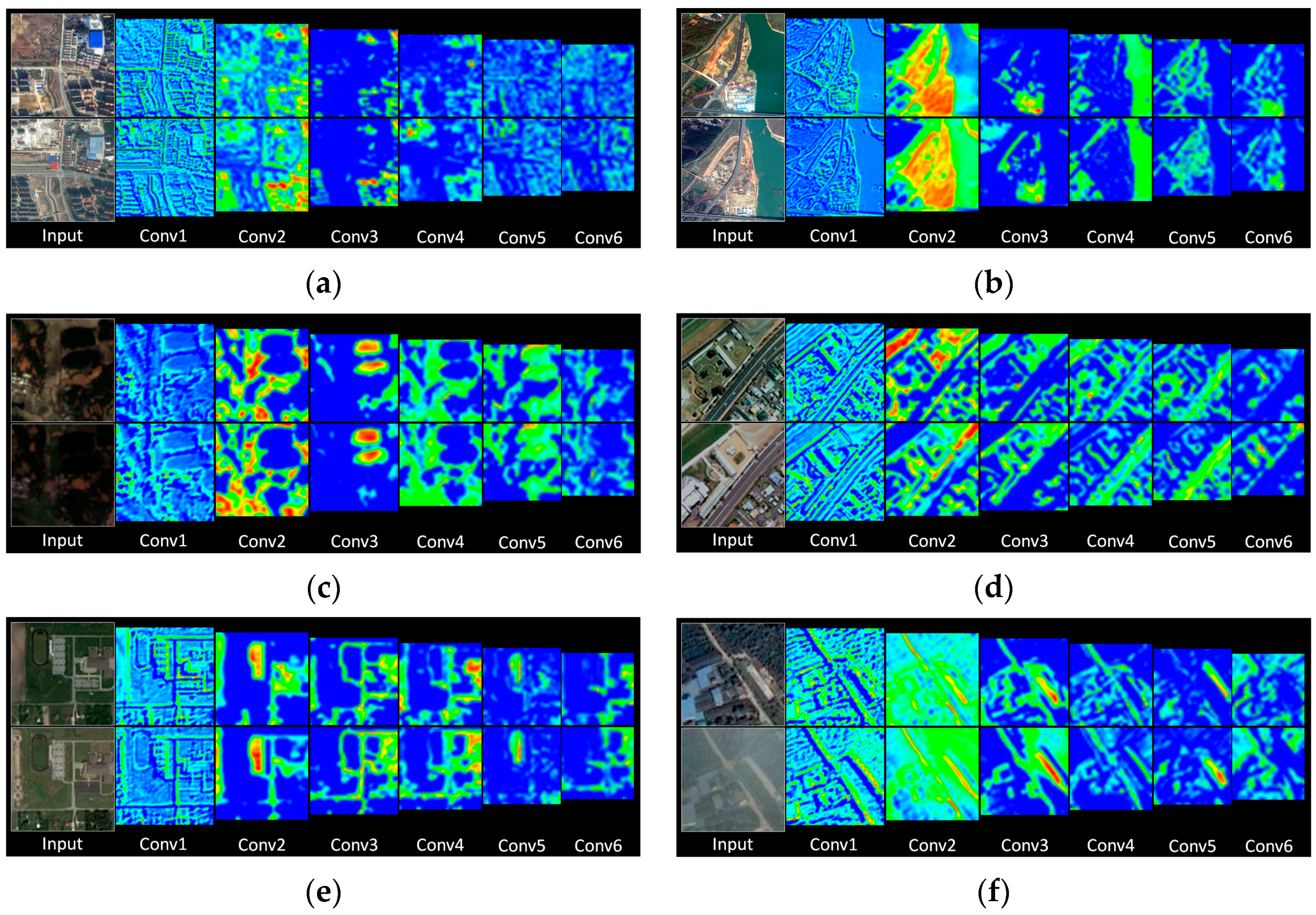
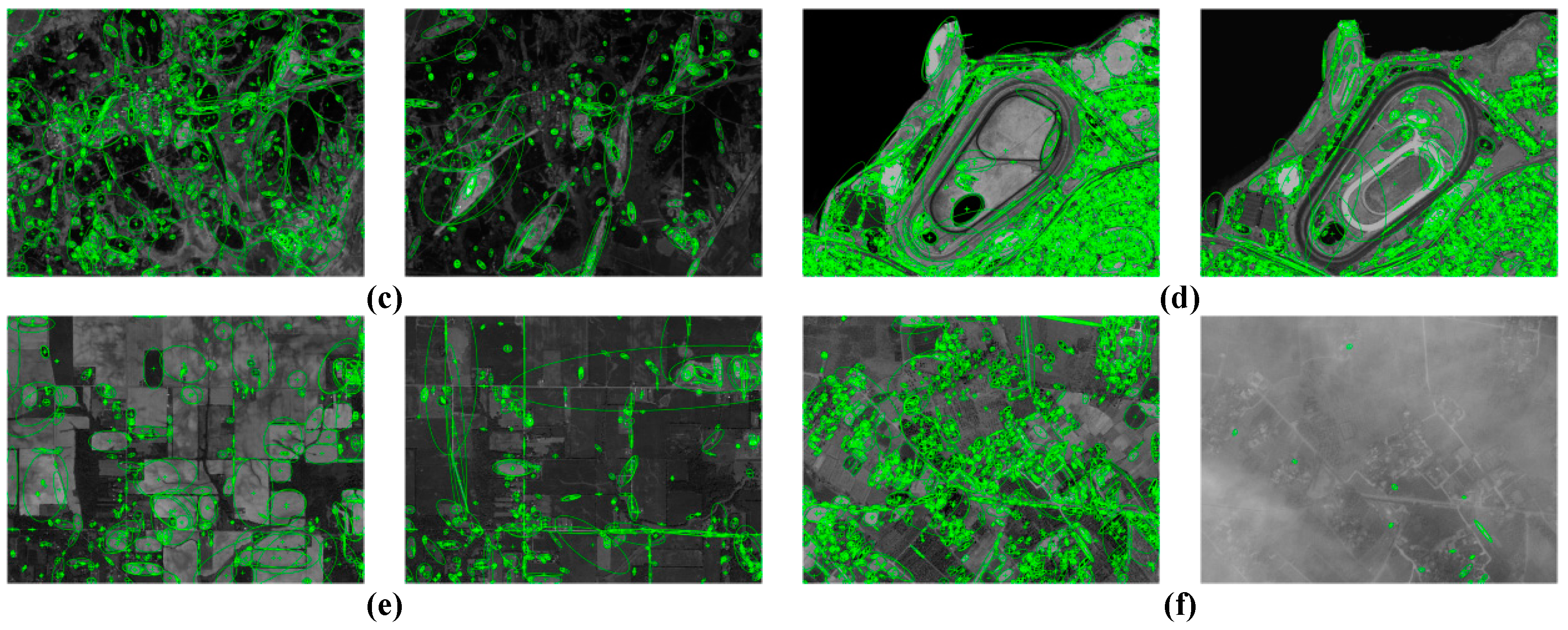
3.3. Feature Visualization
3.4. Evaluation Criteria of Matching Performance
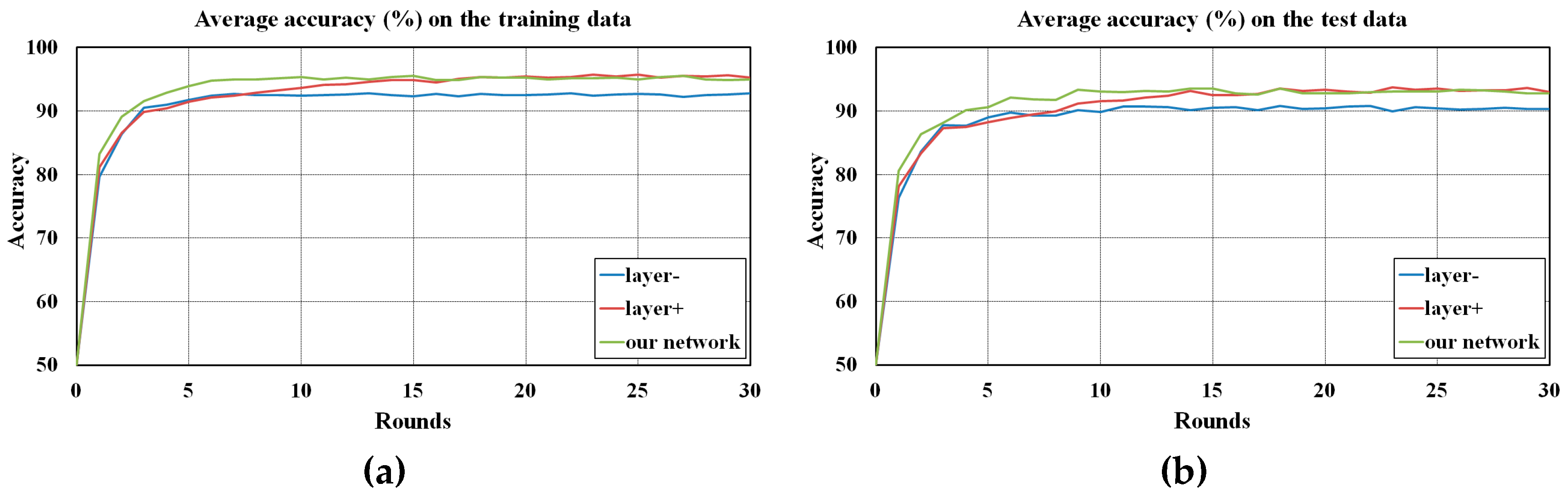
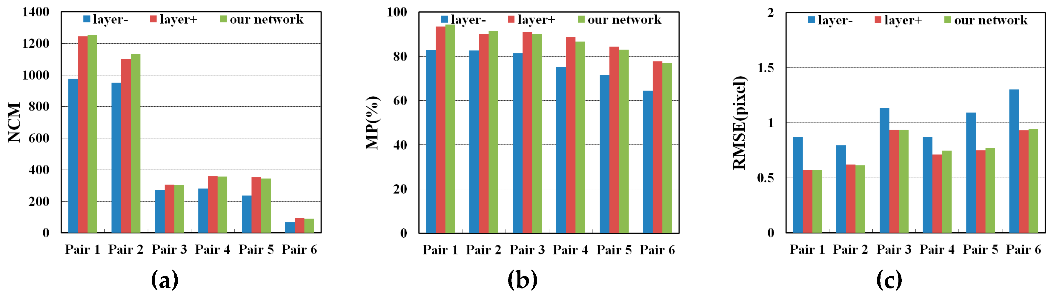
3.5. Comparison of SCNNs with Different Numbers of Layers
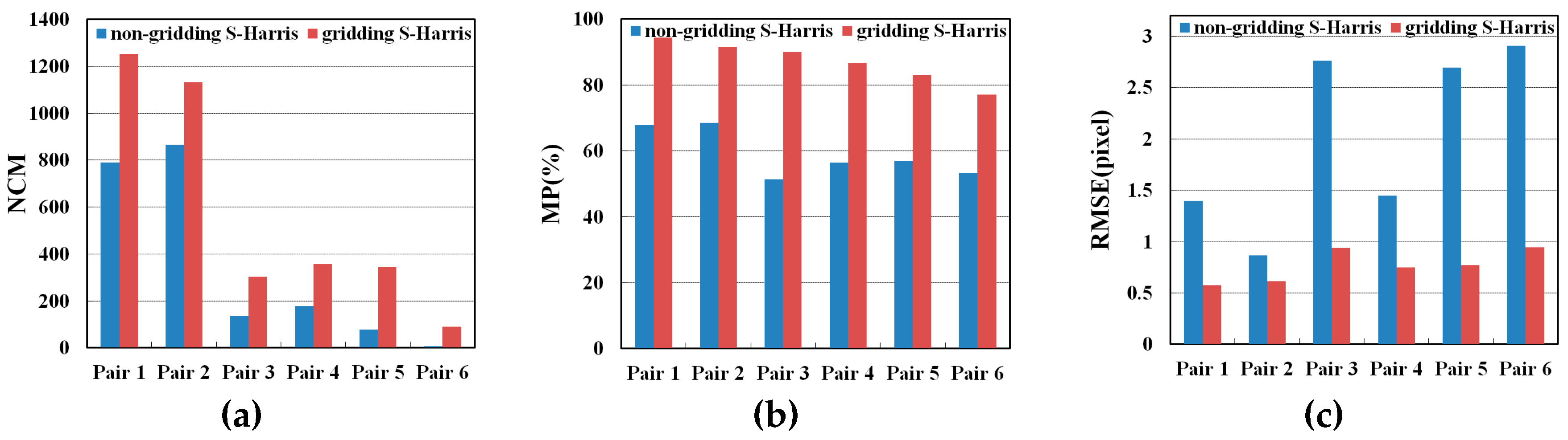
3.6. Comparison between Gridding and Non-Gridding S-Harris
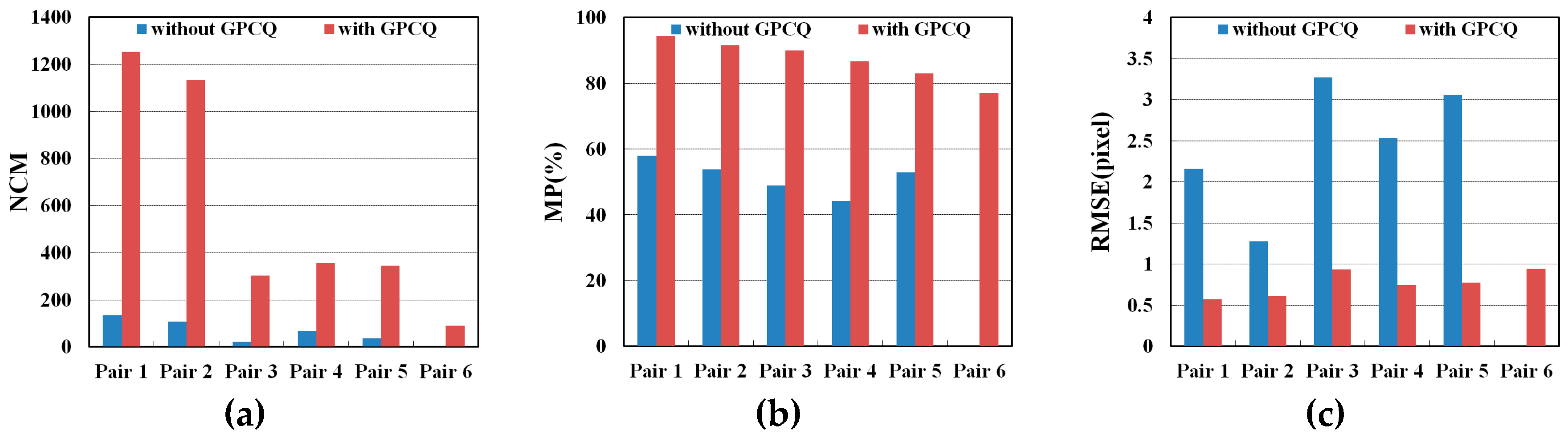
3.7. Evaluation of GPCQ
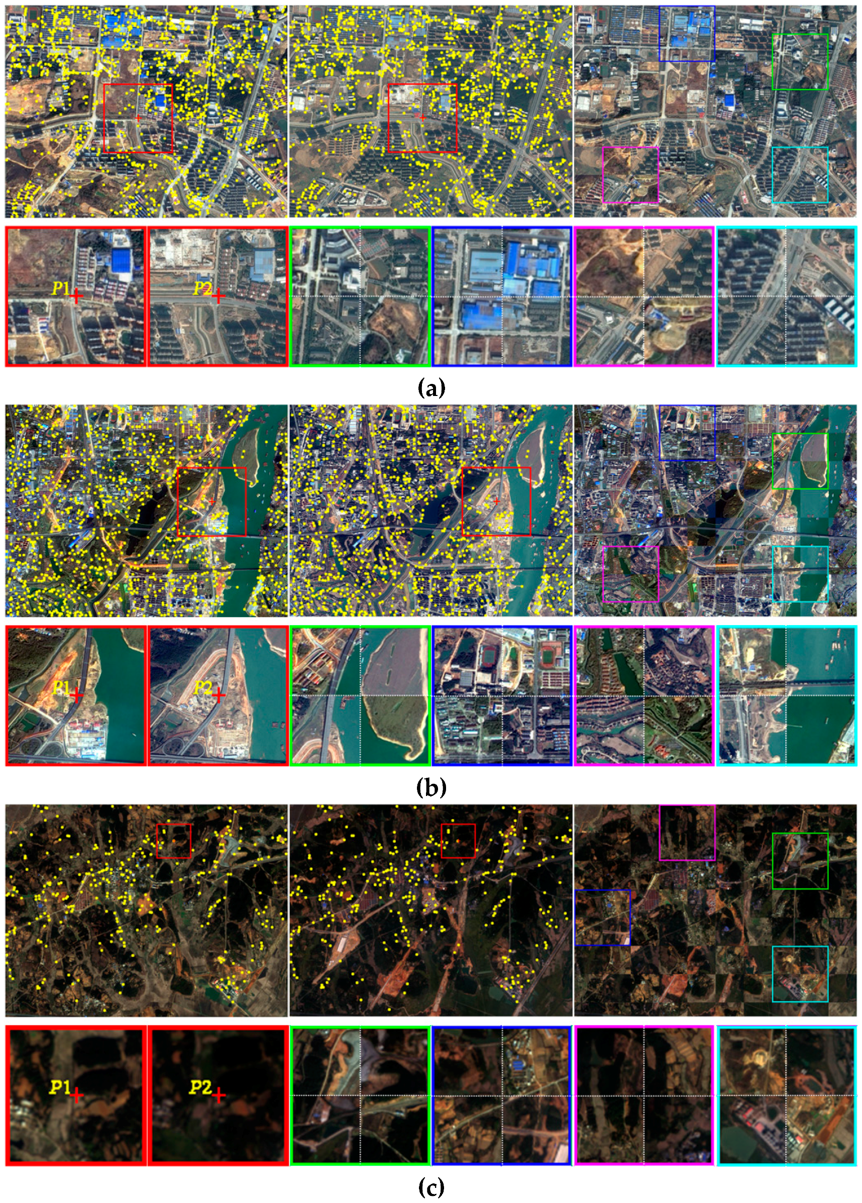
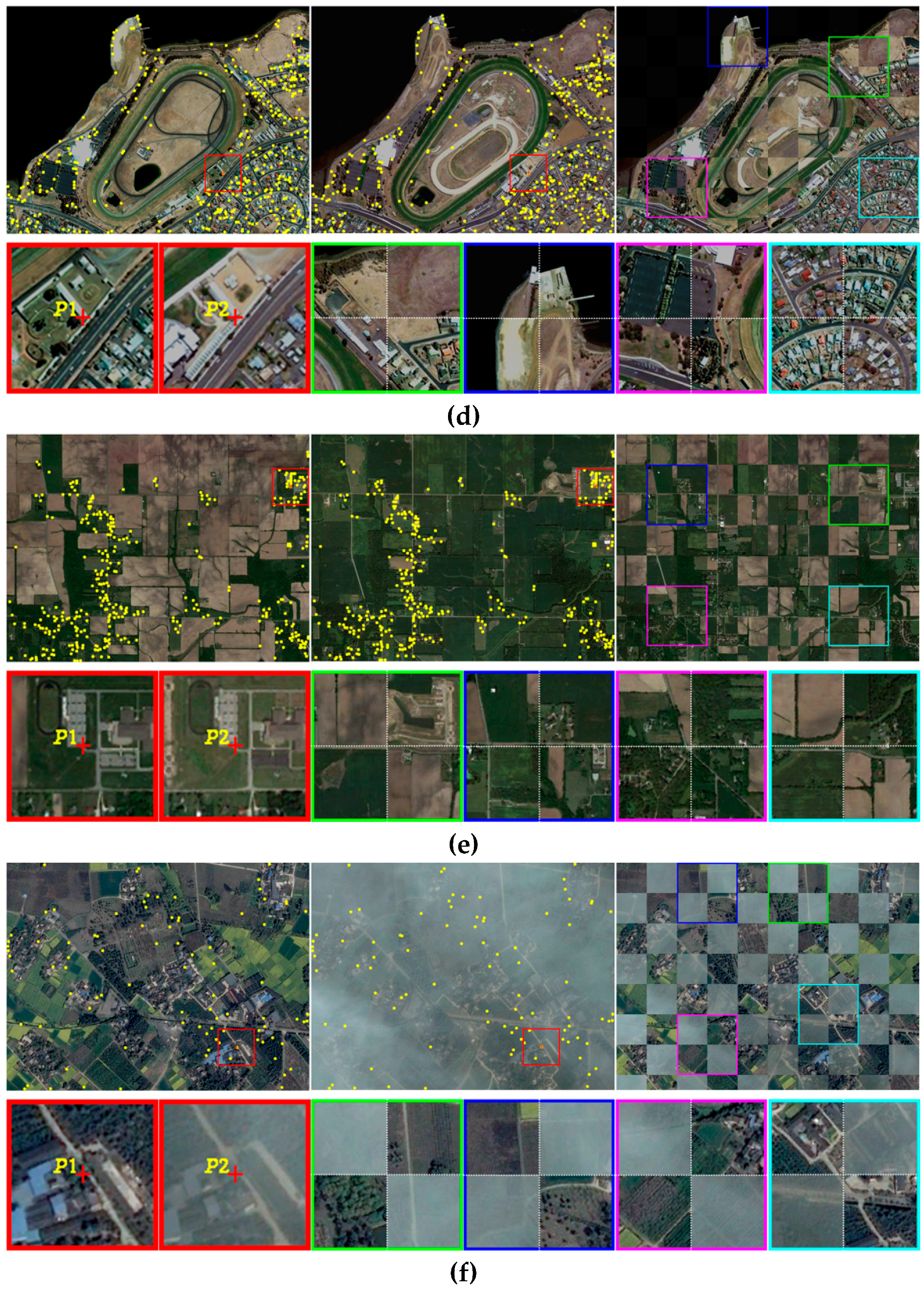
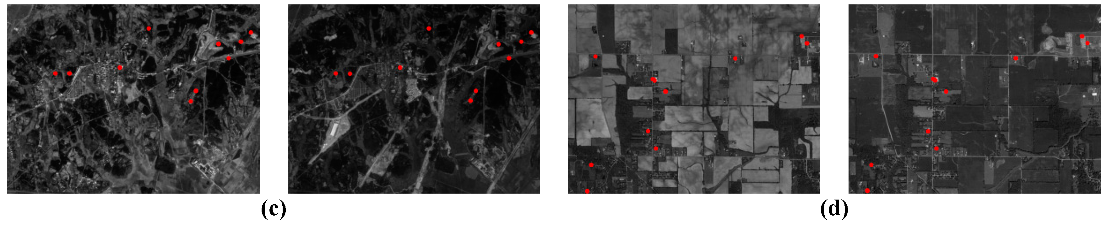
3.8. Performance Evaluation of the Proposed Matching Framework
4. Conclusions
Acknowledgments
Author Contributions
Conflicts of Interest
References
- Brown, L.G. A survey of image registration techniques. ACM Comput. Surv. 1992, 24, 325–376. [Google Scholar] [CrossRef]
- Maintz, J.B.A.; Viergever, M.A. A survey of medical image registration. Med. Image Anal. 1998, 2, 1–36. [Google Scholar] [CrossRef]
- Zitová, B.; Flusser, J. Image registration methods: A survey. Image Vis. Comput. 2003, 21, 977–1000. [Google Scholar] [CrossRef]
- Dawn, S.; Saxena, V.; Sharma, B. Remote sensing image registration techniques: A survey. In International Conference on Image and Signal Processing; Elmoataz, A., Lezoray, O., Nouboud, F., Mammass, D., Meunier, J., Eds.; Springer-Berlin: Heidelberg, Germany, 2010; Volume 6134, pp. 103–112. [Google Scholar]
- Jiang, J.; Zhang, S.; Cao, S. Rotation and scale invariant shape context registration for remote sensing images with background variations. J. Appl. Remote Sens. 2015, 9, 92–110. [Google Scholar] [CrossRef]
- Yang, K.; Pan, A.; Yang, Y.; Zhang, S.; Ong, S.H.; Tang, H. Remote sensing image registration using multiple image features. Remote Sens. 2017, 9, 581. [Google Scholar] [CrossRef]
- Chen, M.; Habib, A.; He, H.; Zhu, Q.; Zhang, W. Robust feature matching method for SAR and optical images by using Gaussian-Gamma-shaped bi-windows-based descriptor and geometric constraint. Remote Sens. 2017, 9, 882. [Google Scholar] [CrossRef]
- Lowe, D. Object recognition from local scale-invariant features. In Proceedings of the 7th IEEE International Conference on Computer Vision, Kerkyra, Greece, 20–27 September 1999; p. 1150. [Google Scholar]
- Bay, H.; Ess, A.; Tuytelaars, T.; Gool, L.C. Speeded-up robust features (SURF). Comput. Vis. Image Und. 2008, 110, 346–359. [Google Scholar] [CrossRef]
- Bradley, P.E.; Jutzi, B. Improved feature detection in fused intensity-range image with complex SIFT. Remote Sens. 2011, 3, 2076–2088. [Google Scholar] [CrossRef]
- Ke, Y.; Sukthankar, R. PCA-SIFT: A more distinctive representation for local image descriptors. In Proceedings of the IEEE Computer Society Conference on Computer Vision and Pattern Recognition, Washington, DC, USA, 27 June–2 July 2004; pp. 506–513. [Google Scholar]
- Mikolajczyk, K.; Schmid, C. A performance evaluation of local descriptors. IEEE Trans. Pattern Anal. 2005, 27, 1615–1630. [Google Scholar] [CrossRef] [PubMed]
- Morel, J.M.; Yu, G. ASIFT: A new framework for fully affine invariant image comparison. SIAM J. Imaging Sci. 2009, 2, 438–469. [Google Scholar] [CrossRef]
- Li, Q.; Wang, G.; Liu, J.; Chen, S. Robust scale-invariant feature matching for remote sensing image registration. IEEE Geosci. Remote Sens. Lett. 2009, 6, 287–291. [Google Scholar]
- Brook, A.; Bendor, E. Automatic registration of airborne and spaceborne images by topology map matching with SURF processor algorithm. Remote Sens. 2011, 3, 65–82. [Google Scholar] [CrossRef]
- Chen, Q.; Wang, S.; Wang, B.; Sun, M. Automatic registration method for fusion of ZY-1-02C satellite images. Remote Sens. 2013, 6, 157–279. [Google Scholar] [CrossRef]
- Cai, G.R.; Jodoin, P.M.; Li, S.Z.; Wu, Y.D.; Su, S.Z. Perspective-SIFT: An efficient tool for low-altitude remote sensing image registration. Signal Process. 2013, 93, 3088–3110. [Google Scholar] [CrossRef]
- Li, J.; Hu, Q.; Ai, M. Robust feature matching for remote sensing image registration based on lq-estimator. IEEE Geosci. Remote Sens. Lett. 2016, 13, 1989–1993. [Google Scholar] [CrossRef]
- Zagoruyko, S.; Komodakis, N. Learning to compare image patches via convolutional neural networks. In Proceedings of the IEEE Conference on Computer Vision and Pattern Recognition (CVPR), Boston, MA, USA, 7–12 June 2015; pp. 4353–4361. [Google Scholar]
- Shi, X.; Jiang, J. Automatic registration method for optical remote sensing images with large background variations using line segments. Remote Sens. 2016, 8, 426. [Google Scholar] [CrossRef]
- Altwaijry, H.; Trulls, E.; Hays, J.; Fua, P.; Belongie, S. Learning to match aerial images with deep attentive architecture. In Proceedings of the IEEE Conference on Computer Vision and Pattern Recognition (CVPR), Seattle, WA, USA, 27–30 June 2016; pp. 3539–3547. [Google Scholar]
- Chen, L.; Rottensteiner, F.; Heipke, C. Invariant descriptor learning using a Siamese convolutional neural network. In Proceedings of the ISPRS Annals of the Photogrammetry, Remote Sensing and Spatial Information Sciences, Prague, Czech Republic, 12–19 July 2016; pp. 11–18. [Google Scholar]
- Simo-Serra, E.; Trulls, E.; Ferraz, L.; Kokkinos, I.; Fua, P.; Moreno-Noguer, F. Discriminative learning of deep convolutional feature point descriptors. In Proceedings of the IEEE International Conference on Computer Vision, Santiago, Chile, 7–13 December 2015; pp. 118–126. [Google Scholar]
- Ahmed, E.; Jones, M.; Marks, T.K. An improved deep learning architecture for person re-identificaiton. In Proceedings of the IEEE Conference on Computer Vision and Pattern Recognition, Boston, MA, USA, 7–12 June 2015; pp. 3908–3916. [Google Scholar]
- Melekhov, I.; Kannala, J.; Rahtu, E. Siamese Network Features for Image Matching. In Proceedings of the 23rd International Conference on Pattern Recognition, Cancun, Mexico, 4–8 December 2016; pp. 378–383. [Google Scholar]
- Fischler, M.A.; Bolles, R.C. Random sample consensus: a paradigm for model fitting with applications to image analysis and automated cartography. ACM 1981, 24, 381–395. [Google Scholar] [CrossRef]
- Brum, A.G.V.; Pilchowski, H.U.; Faria, S.D. Attitude determination of spacecraft with use of surface imaging. In Proceedings of the 9th Brazilian Conference on Dynamics Control and their Applications (DICON’10), Serra Negra, Brazil, 7–11 June 2010; pp. 1205–1212. [Google Scholar]
- Kouyama, T.; Kanemura, A.; Kato, S.; Imamoglu, N.; Fukuhara, T.; Nakamura, R. Satellite attitude determination and map projection based on robust image matching. Remote Sens. 2017, 9, 90. [Google Scholar] [CrossRef]
- Zhang, H.; Sun, K.; Li, W. Object-oriented shadow detection and removal from urban high-resolution remote sensing images. IEEE Trans. Geosci. Remote Sens. 2014, 52, 6972–6982. [Google Scholar] [CrossRef]
- Cheng, Q.; Shen, H.; Zhang, L.; Li, P. Inpainting for remotely sensed images with a multichannel nonlocal total variation model. IEEE Trans. Geosci. Remote Sens. 2014, 52, 175–187. [Google Scholar] [CrossRef]
- Ioffe, S.; Szegedy, C. Batch normalization: Accelerating deep network training by reducing internal covariate shift. In Proceedings of the 32nd International Conference on Machine Learning (ICML–15), Lille, France, 6–11 July 2015. [Google Scholar]
- Merkle, N.; Luo, W.; Auer, S.; Müller, R.; Urtasun, R. Exploiting deep matching and SAR data for the geo-localization accuracy improvement of optical satellite images. Remote Sens. 2017, 9, 586. [Google Scholar] [CrossRef]
- Harris, C. A combined corner and edge detector. In Proceedings of the 4th Alvey Vision Conference, Manchester, UK, 31 August–2 September 1988; pp. 147–151. [Google Scholar]
- Brown, M.; Hua, G.; Winder, S. Discriminative learning of local image descriptors. IEEE Trans. Pattern Anal. 2011, 33, 43–57. [Google Scholar] [CrossRef] [PubMed]
- Matas, J.; Chum, O.; Urban, M.; Pajdla, T. Robust wide baseline stereo from maximally stable extremal regions. In Proceedings of the British Machine Vision Conference, Cardiff, UK, 2–5 September 2002; pp. 384–396. [Google Scholar]


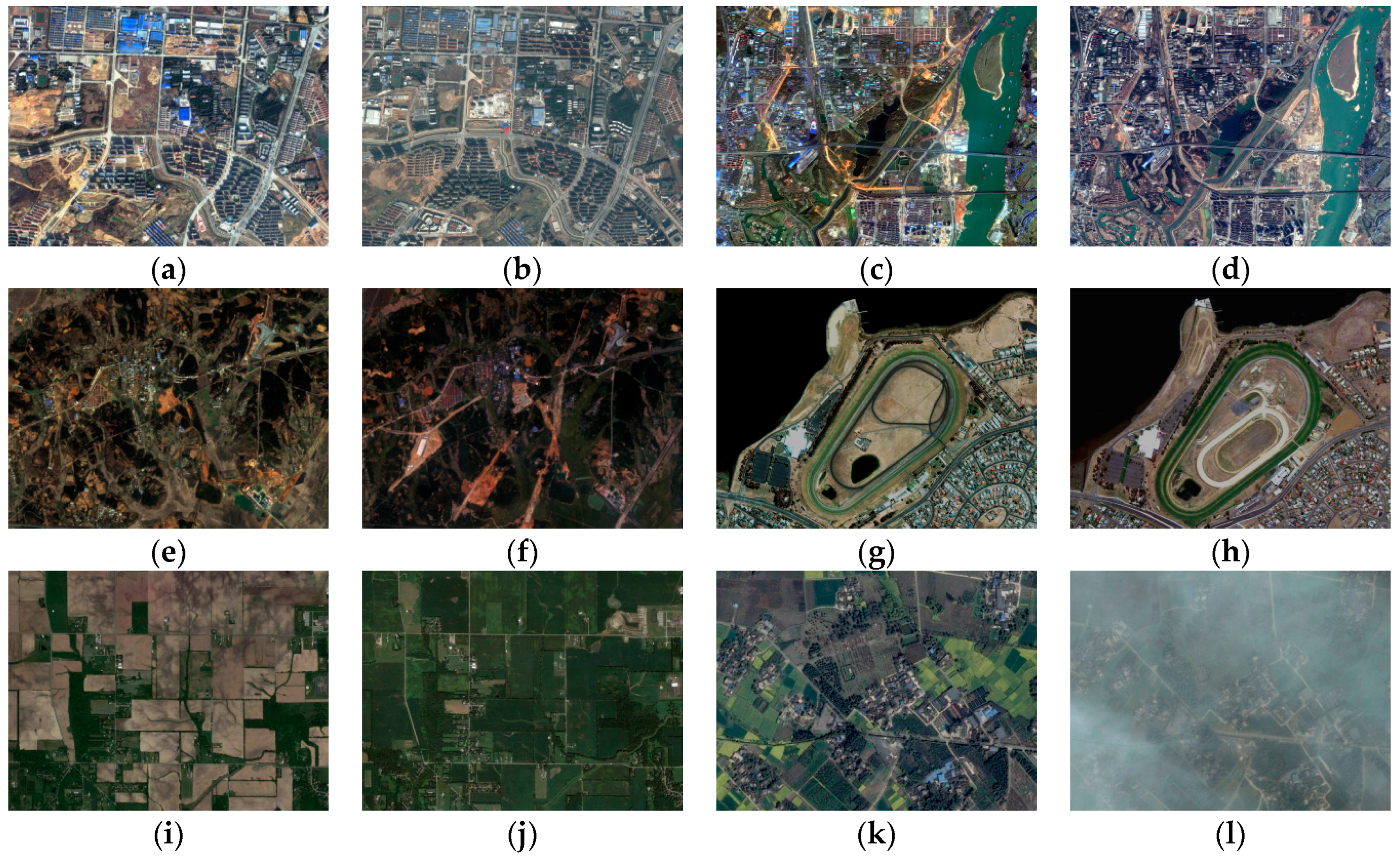
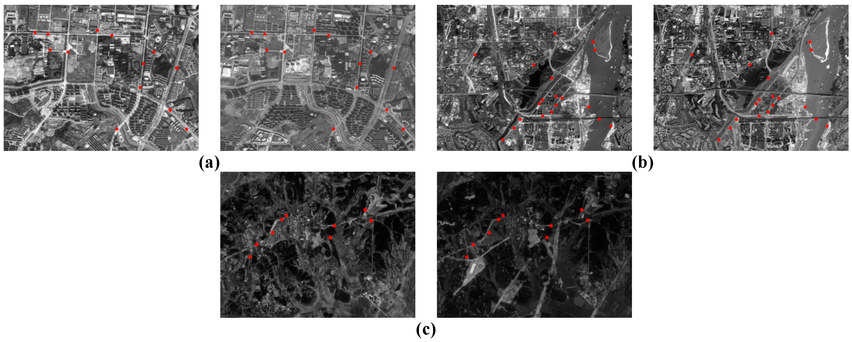
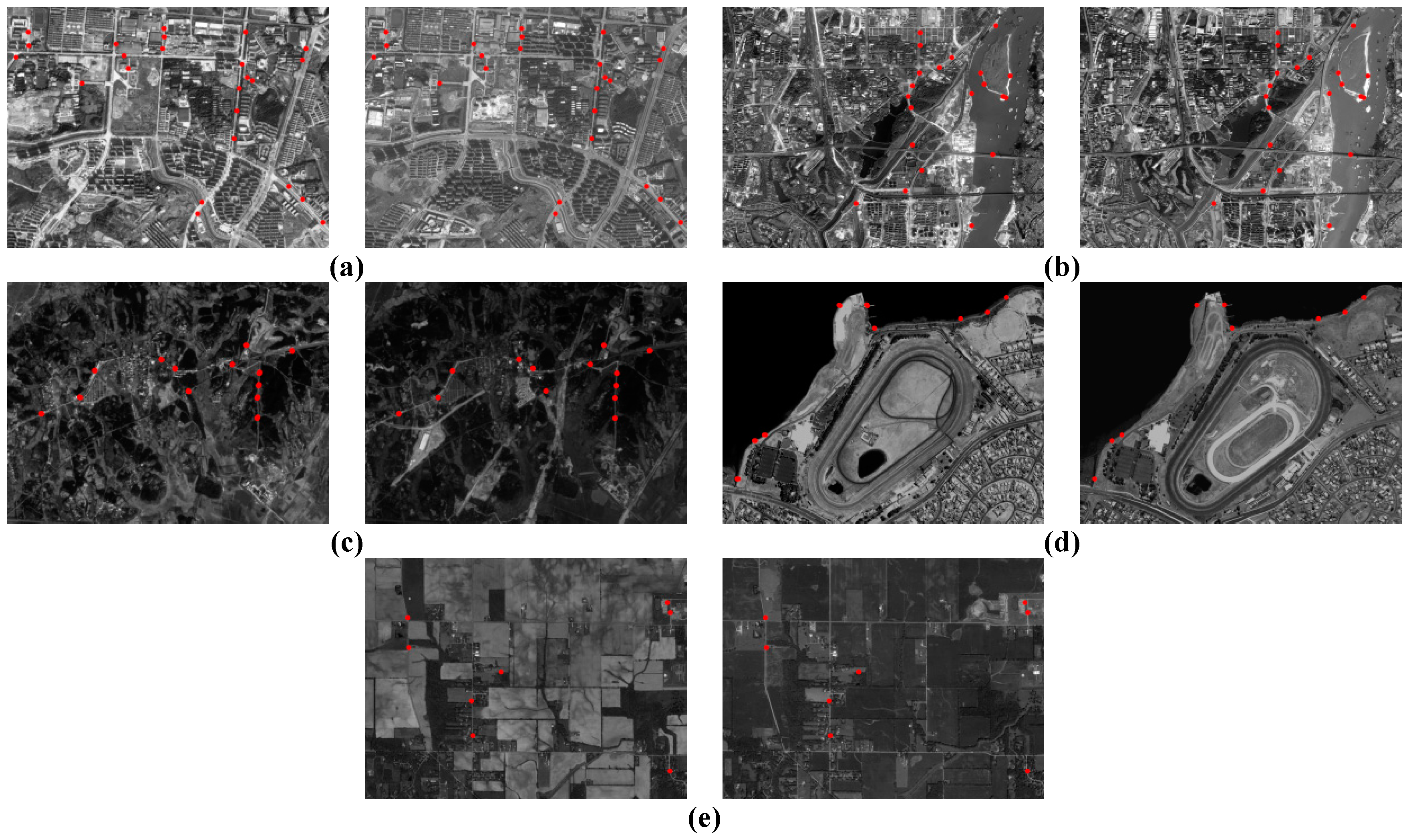
| Pairs | Image Number | Year | Image Source | Image Size (Unit: Pixel) | Spatial Resolution (Unit: Meter) |
|---|---|---|---|---|---|
| Pair 1 | (a) | 2013 | ZY3 | 1000 × 750 | 2.10 |
| (b) | 2017 | Google Earth | 1765 × 1324 | 1.19 | |
| Pair 2 | (c) | 2015 | GF1 | 1972 × 1479 | 2.00 |
| (d) | 2017 | Google Earth | 3314 × 2485 | 1.19 | |
| Pair 3 | (e) | 2013 | ZY3 | 780 × 585 | 5.80 |
| (f) | 2015 | GF1 | 565 × 424 | 8.00 | |
| Pair 4 | (g) | 2003 | IKONOS | 1190 × 893 | 1.00 |
| (h) | 2017 | Google Earth | 1000 × 750 | 1.19 | |
| Pair 5 | (i) | 2016 | Google Earth | 1936 × 1452 | 1.19 |
| (j) | 2016 | Google Earth | 1936 × 1452 | 1.19 | |
| Pair 6 | (k) | 2015 | Google Earth | 1686 × 1264 | 1.19 |
| (l) | 2016 | Google Earth | 1686 × 1264 | 1.19 |
| Image Pair | Matching Methods | ||||
|---|---|---|---|---|---|
| SIFT | Jiang | Shi | Zagoruyko | Proposed | |
| Pair 1 | 93 | 13 | 24 | 39 | 1253 |
| Pair 2 | 69 | 19 | 25 | 71 | 1132 |
| Pair 3 | 10 | 9 | 13 | 0 | 303 |
| Pair 4 | 0 | 0 | 9 | 0 | 356 |
| Pair 5 | 14 | 0 | 7 | 0 | 345 |
| Pair 6 | 0 | 0 | 0 | 0 | 91 |
| Image Pair | Matching Methods | ||||
|---|---|---|---|---|---|
| SIFT | Jiang | Shi | Zagoruyko | Proposed | |
| Pair 1 | 51.8% | 68.3% | 73.6% | 85.7% | 94.3% |
| Pair 2 | 54.2% | 76.2% | 80.4% | 84.6% | 91.6% |
| Pair 3 | 42.6% | 71.5% | 77.8% | 0.0% | 89.9% |
| Pair 4 | 0.0% | 0.0% | 79.1% | 0.0% | 86.7% |
| Pair 5 | 60.4% | 0.0% | 66.2% | 0.0% | 82.9% |
| Pair 6 | 0.0% | 0.0% | 0.0% | 0.0% | 77.1% |
| Image Pair | Matching Methods | ||||
|---|---|---|---|---|---|
| SIFT | Jiang | Shi | Zagoruyko | Proposed | |
| Pair 1 | 0.8732 | 2.9674 | 2.1536 | 0.9657 | 0.5736 |
| Pair 2 | 0.9485 | 2.1453 | 2.4665 | 0.9054 | 0.6143 |
| Pair 3 | 2.4153 | 2.7478 | 2.5833 | Null | 0.9372 |
| Pair 4 | Null | Null | 2.0751 | Null | 0.7476 |
| Pair 5 | 1.7834 | Null | 2.9887 | Null | 0.7732 |
| Pair 6 | Null | Null | Null | Null | 0.9426 |
© 2018 by the authors. Licensee MDPI, Basel, Switzerland. This article is an open access article distributed under the terms and conditions of the Creative Commons Attribution (CC BY) license (http://creativecommons.org/licenses/by/4.0/).
Share and Cite
He, H.; Chen, M.; Chen, T.; Li, D. Matching of Remote Sensing Images with Complex Background Variations via Siamese Convolutional Neural Network. Remote Sens. 2018, 10, 355. https://doi.org/10.3390/rs10020355
He H, Chen M, Chen T, Li D. Matching of Remote Sensing Images with Complex Background Variations via Siamese Convolutional Neural Network. Remote Sensing. 2018; 10(2):355. https://doi.org/10.3390/rs10020355
Chicago/Turabian StyleHe, Haiqing, Min Chen, Ting Chen, and Dajun Li. 2018. "Matching of Remote Sensing Images with Complex Background Variations via Siamese Convolutional Neural Network" Remote Sensing 10, no. 2: 355. https://doi.org/10.3390/rs10020355
APA StyleHe, H., Chen, M., Chen, T., & Li, D. (2018). Matching of Remote Sensing Images with Complex Background Variations via Siamese Convolutional Neural Network. Remote Sensing, 10(2), 355. https://doi.org/10.3390/rs10020355