Monitoring Rice Phenology Based on Backscattering Characteristics of Multi-Temporal RADARSAT-2 Datasets

Abstract

Accurate estimation and monitoring of rice phenology is necessary for the management and yield prediction of rice. The radar backscattering coefficient, one of the most direct and accessible parameters has been proved to be capable of retrieving rice growth parameters. This paper aims to investigate the possibility of monitoring the rice phenology (i.e., transplanting, vegetative, reproductive, and maturity) using the backscattering coefficients or their simple combinations of multi-temporal RADARSAT-2 datasets only. Four RADARSAT-2 datasets were analyzed at 30 sample plots in Meishan City, Sichuan Province, China. By exploiting the relationships of the backscattering coefficients and their combinations versus the phenology of rice, HH/VV, VV/VH, and HH/VH ratios were found to have the greatest potential for phenology monitoring. A decision tree classifier was applied to distinguish the four phenological phases, and the classifier was effective. The validation of the classifier indicated an overall accuracy level of 86.2%. Most of the errors occurred in the vegetative and reproductive phases. The corresponding errors were 21.4% and 16.7%, respectively.

1. Introduction

Rice is one of the most important cultivated grain crops and is the staple food of nearly half of the world’s population [1]. Approximately 969 million metric tons of rice were produced worldwide in 2010 and about one-third of them were from China [2]. Effective management of rice cultivation that includes the prediction of the growth conditions and stages of rice accurately and timely is crucial to food security and social stability. Thus, the accurate acquisition of rice phenological information is an important component of the farming management system [3,4,5]. This type of information provides an accurate knowledge on the status of rice plants, leading to different cultivation practices (e.g., irrigation, fertilization, or harvest) [6,7,8]. Rice phenology is also used as an input in the rice growth and yield prediction models, ecosystem productivity models, and land surface process models [6,9,10].

The phenological stages of crops can be measured using a field survey, simulation by bioclimatic models, or detection with remotely sensed data [7,11]. Conventional ground-based rice phenology monitoring provides accurate in situ information if properly designed and executed. The monitoring is, unfortunately, linked to enormous costs of time, money, and man-power [12,13], and is not practical at a large spatial extent and for long-term monitoring and analysis. During the past decades, a series of spaceborne optical and synthetic aperture radar (SAR) sensors with a high or moderate resolution have been launched, and new approaches for the phenology study have been conceived. Optical data such as the Moderate Resolution Imaging Spectroradiometer (MODIS) [3,14,15,16,17], and HJ-1 and Landsat data [18] are used to effectively estimate rice phenology. However, an optical sensor is vulnerable to the variation of atmospheric conditions and cloud covers. Compared to the optical sensor, SAR has an all-time and all-weather imaging capability. SAR data are sensitive to surface features [19] and inundated/un-inundated rice fields [20]. Thus, SAR plays an important role in the monitoring of rice in cloudy or foggy areas.

Many researchers have obtained successful results in rice planting monitoring using X-band sensors (e.g., COSMO-SkyMed and TerraSAR-X) [13,21,22,23,24,25] and C-band sensors (e.g., Envisat-ASAR, RADARSAT-2, and Sentinel-1) [19,20,26,27,28]. After the successful launch of spaceborne SARs with short revisit periods (compared to the main phenological phases of rice with a short duration, e.g., about 16 days of reproductive phase) or polarimetric mode, the acquisition of timely and accurate information about the rice condition during the growing period became readily possible. Lopez-Sanchez et al. [5] used TerraSAR-X data to retrieve rice phenological phases with the correlation and phase difference between co-polar channels and parameters provided by polarimetric decomposition techniques. The potential of TerraSAR-X data for rice phenology monitoring has been well documented [5,7,21,22,23]. However, the penetration depth into the canopy is shallow for radar energy at a high frequency compared to that at a low frequency [29]. Therefore, the backscattering at X-band may provide less information on the structure of rice plants than that at C-band [29,30]. Tian et al. [28] have used C-band Sentinel-1A and Landsat-8 data to map multi-season paddy rice based on backscattering coefficients (${\mathsf{\sigma }}^0$) and the normalized difference vegetation index (NDVI) with a K-Means unsupervised classifier. The high temporal resolution, six days using the two-satellite constellation of Sentinel-1, makes Sentinel-1 data suitable for rice monitoring. However, Sentinel-1 SAR can only provide single or dual-pol data. Since various polarized radar backscattering coefficients respond to rice plants differently [6,25,31], quad-polarized data (e.g., RADARSAT-2) can supply more comprehensive information on rice growth status than single and dual-polarized data.

Although the revisit time of TerraSAR-X (11 days) and Sentinel-1 (six or 12 days) is shorter than that of RADARSAT-2, whose revisit period is 24 days, RADARSAT-2 can still observe a rice field at least four times during the typical cultivation cycle of rice [6,9]. Because of the different cultivation management (e.g., transplanting time and fertilization) and rice varieties in individual fields, the pace of rice phenology evolution varies at field-by-field levels [11]. Thus, it is acceptable to observe the fields in each of the four principle phenological phases (i.e., transplanting, vegetative, reproductive, and maturity) once in 24 days or longer. Besides, RADARSAT-2 provides quad-polarization (VH, VV, HH, HV) data, and is very effective in retrieving rice canopy parameters and estimating biomass that are linked to the crop yield [30,32]. As a result, the sensor has become an ideal data source for rice phenology monitoring. Lopez-Sanchez et al. [6] analyzed RADARSAT-2 data and proposed a retrieval algorithm with radar target decomposition and compact polarimetric (CP) variables. Francis et al. [27] found that the combination of the alpha angle and beta angle derived from the Cloude-Pottier decomposition of RADARSAT-2 data provided satisfactory estimations of the crop phenology. Yang et al. [9] used RADARSAT-2 data to simulate the CP SAR data for identifying seven phenological phases of rice fields. However, most of these studies require various indirect parameters like the CP and target decomposition parameters. The retrieval processes are generally complex including filtering and image classification that may create new uncertainties in data analysis.

Of the SAR polarimetric parameters (i.e., amplitude and phase data), the backscattering coefficient is proportional to the square of amplitude and is the most basic one [5]. Many researches have demonstrated that the rice backscattering coefficient alone is sensitive to plant height, biomass, and leaf area index (LAI) [19,20,33,34,35,36,37]. These plant parameters are highly correlated with rice phenology development, showing a great potential to monitor rice phenology. However, the observed correlation between rice biophysical variables and certain polarizations [25,30] can be temporally unstable. This is caused by changes of the electromagnetic interactions between radar waves and rice scattering components as the plant grows and different polarization responses to the changes [20]. Li et al. [31] used multi-temporal, quad-polarization RADARSAT-2 data to establish empirical regression models to link rice biophysical parameters to backscattering coefficients. The optimal polarization to estimate biophysical variables was a function of different stages, which suggests a piecewise fitting strategy using different polarizations at different growing stages. As rice plants develop during a growing season and biophysical variables change during different phenological phases, ${\mathsf{\sigma }}^0$ acquired at different phases should be clustered in the domains of polarizations and/or combinations of polarizations, making the decision tree strategy with particular thresholds theoretically feasible for the separation of phenological phases. Therefore, the objective of this study is to use only radar backscattering coefficients and their combinations derived from multi-temporal and full-polarized RADARSAT-2 datasets for rice phenology monitoring. The focus of the study is to utilize a simple decision tree model for the characterization of rice phenology in the feature space of backscattering coefficients of multi-temporal RADARSAT-2 datasets.

2. Materials and Methods

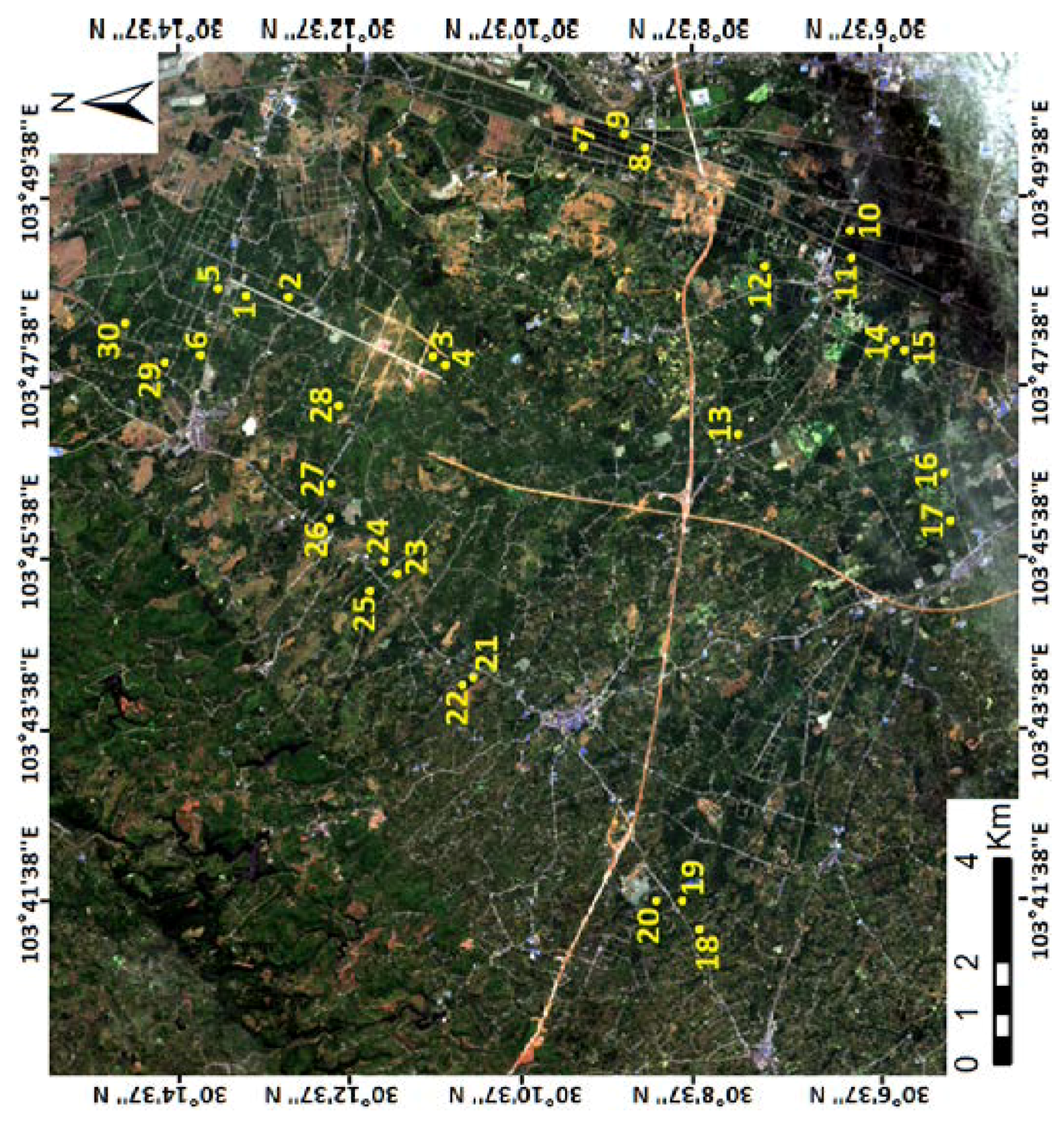
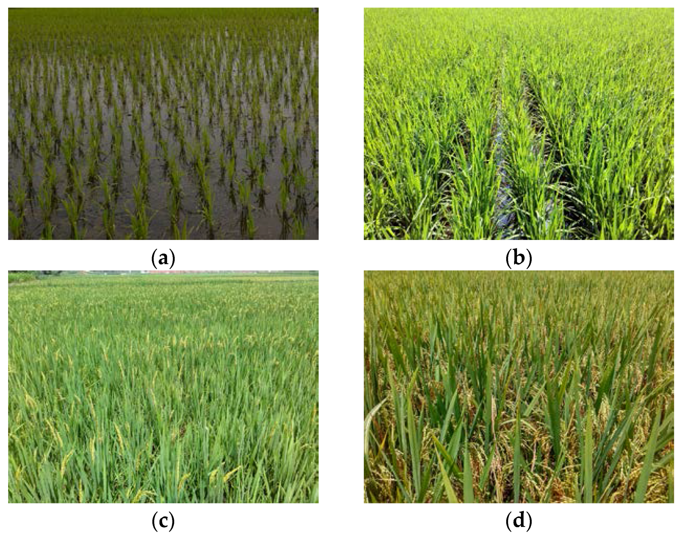
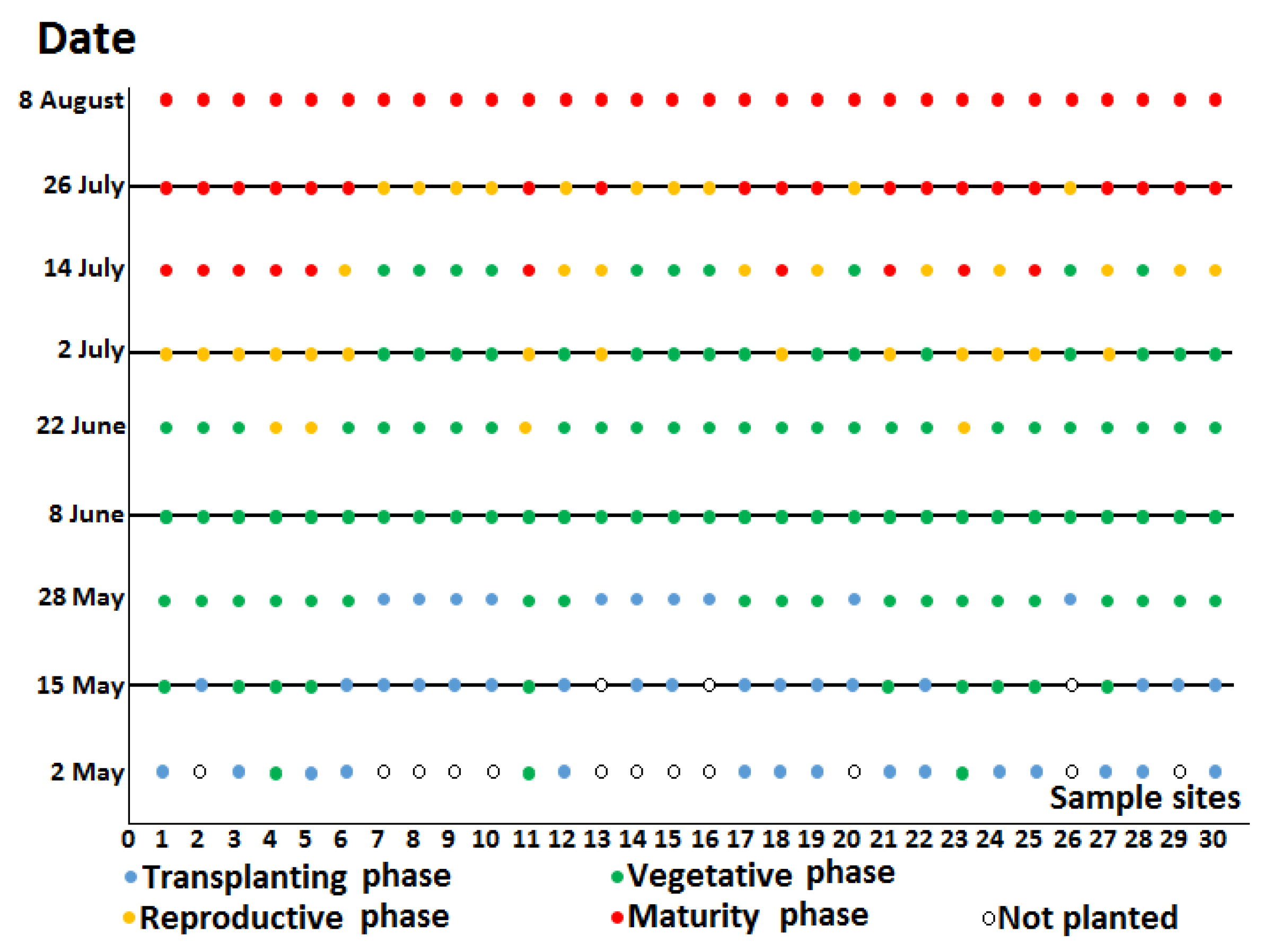
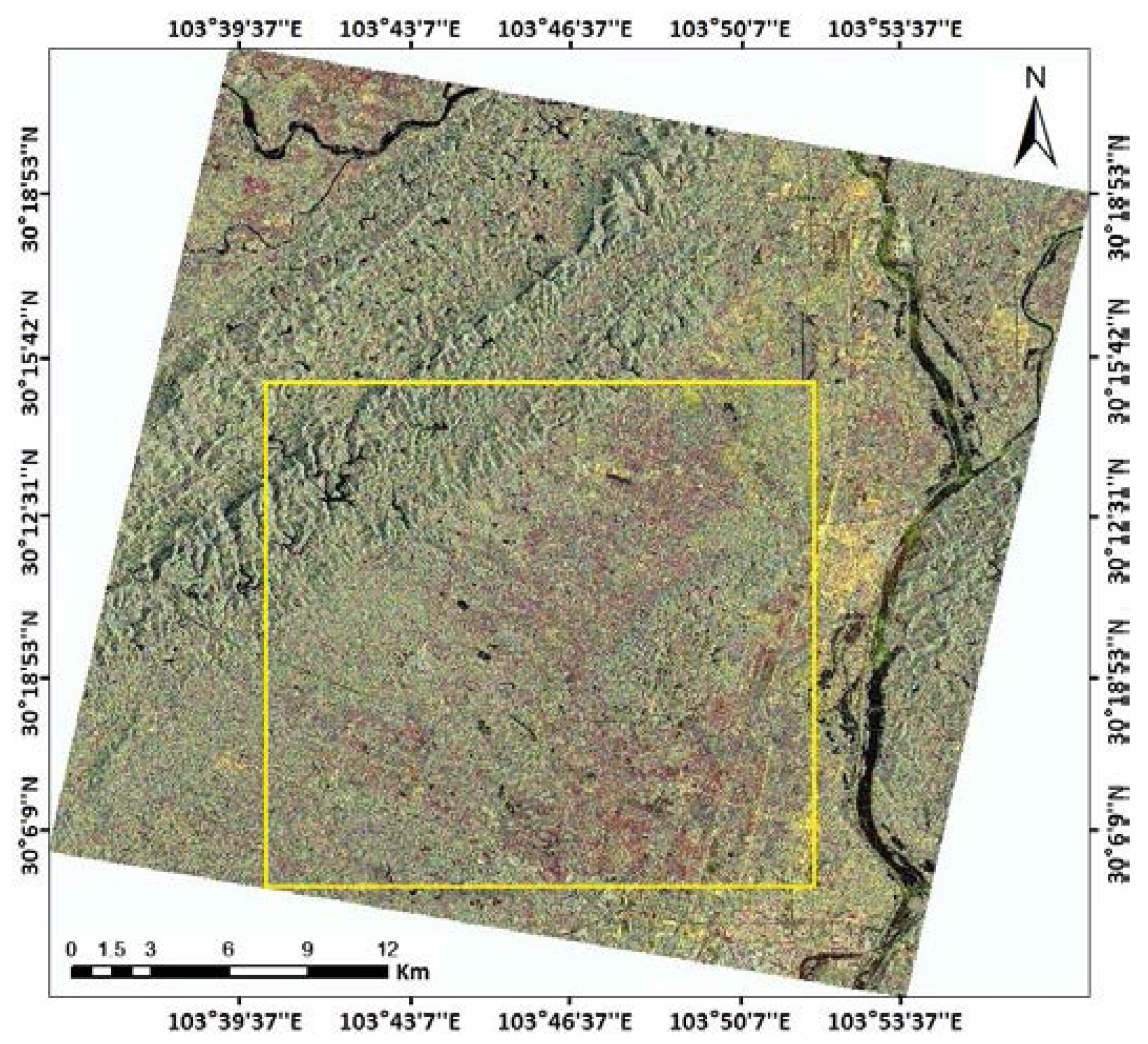
2.1. Study Area and Field Observation

Chengdu Basin, southwestern China, is a main rice production region in China, where rice is cultivated once per year. The growing season is typically from May to August. Under the influence of subtropical monsoon climate and basin terrain characteristics, the sky is constantly cloudy and rainy for most of the growing period. The study area, Meishan City, is located in the western part of Chengdu Basin. Field observations were conducted about every 12 days from 2 May to 8 August in 2016 at 30 sample sites (Figure 1). Each site was at least 50m wide and 50m long. A hand-held GPS unit was used to locate the sites and 11 ground control points (GCPs), which were used to geo-reference the radar data and sites. Plant height, stem diameter, length and width of leaves, and tiller and ear number were measured to identify rice phenology.

2.2. Rice Phenology

Rice phenology can be divided into three main phases: vegetative, reproductive, and maturity, according to the widely-used Biologische Bundesanstalt, Bundessortenamt und CHemische scale (a German scale used to identify the phenological development stages of cereals, BBCH) [13,21,38]. The principal phases and corresponding numerical ranges are shown in

Table 1. Description of the phenology of cereals using the BBCH Scale.

Principle Phase	BBCH	Name
Vegetative	00–09	Germination
	10–19	Leaf development
	20–29	Tillering
	30–39	Stem elongation
	40–49	Booting
Reproductive	50–59	Heading
	60–69	Flowering
Maturity	70–79	Development of fruit
	80–89	Ripening
	90–99	Senescence
Transplanting	00–19	Transplanting, recovery (rice only)

. Most of the Asian rice cultivars are largely grown under the transplanting procedure, which marks the beginning of a cultivation cycle in fields. Transplanting induces a development stoppage followed by a recovery period that can last about 19 days on average in this study area. Besides, the backscattering properties of a rice paddy during this period can be quite different from other stages in the vegetative phase, as shown later in this study. Therefore, the transplanting phase was extracted from the vegetative phase and specially analyzed.

Four phenological phases, including the transplanting (from stage 0 to 19), vegetative (from stage 20 to 49), reproductive (from stage 50 to 69), and maturity (from stage 70 to 99) phases, are studied. They are distinguishable based on field observations (Figure 2) according to the BBCH scale. Fields at a sample site reach a particular BBCH stage when more than 50% of their plants reach that stage [6]. This criterion is considered in the analyses of the ground measurements and radar images.

According to field observations, the average durations of the transplanting, vegetative, reproductive, and maturity phase were 19, 45, 16, and 30 days, respectively, for fields in 30 sample sites in 2016. The 24-day revisit period of RADARSAT-2 might be too coarse for the monitoring of the phase with 16 or 19 days. However, because of the different cultivation management (e.g., transplanting time and fertilization) and rice varieties, the evolution pace of rice phenology varied at different sites. Accordingly, each phenological phase had an extended span and the corresponding phase can be observed. For example, the reproductive phase lasted about 16 days for most of the fields, but field observations showed that the reproductive phase started from June 22 and ended on July 26 in 2016 (Figure 3).

Table 2. The number of sample sites in different phenological phases when SAR datasets were acquired. On 15 May 2016, fields where three sample sites were located were not planted yet.

		Acquisition Dates of SAR Datasets
		15 May	8 June	2 July	26 July
Fields hase	Transplanting	17	0	0	0
	Vegetative	10	30	16	0
	Reproductive	0	0	14	10
	Maturity	0	0	0	20

shows the typical growth rhythm extracted from the field measurement. About 63%, 100%, 47%, and 67% of sample sites were, respectively, in transplanting, vegetative, reproductive, and maturity phases on the dates of RADARSAT-2 acquisitions in 2016 (Table 2). It should be noted that on 15 May 2016, fields where three sample sites were located were not planted yet.

2.3. RADARSAT-2 Data Preprocessing

Four fine quad-polarized single-look complex (SLC) RADARSAT-2 SAR images were acquired between May and July of 2016 (Table 2). The revisit period was 24 days. The images had a nominal spatial resolution of 5.4 m in the slant range direction and 7.9 m in the azimuth direction. The swath width of the image was about 25 km. The incidence angle ranged from 31° at near range to 33° at far range. The Next ESA SAR Toolbox (NEST) software (https://earth.esa.int/web/nest/downloads/) was utilized for data preprocessing including radiometric correction, multilooking, geometry reprojection, speckle filtering, and multi-temporal coregistration. A color composite is shown in Figure 4. Backscattering coefficients (linear scale) of all images on four polarizations (VH, VV, HH, and HV) were extracted for 30 sample sites. As described previously, each sample site is at least 50 m wide and 50 m long and the preprocessed images have a pixel size of 11.6 m × 11.6 m, which means that each sample site has at least 4 by 4 or 16 pixels. Therefore, the mean value of the backscattering coefficients within a sample site was calculated to represent the backscatter properties of that site.

Cross-polarization VH data and HV data were the same. Thus, only VH, VV, and HH data were used. Previous studies have found that combinations (e.g., addition, subtraction, multiplication, and ratioing) of different polarized backscattering coefficients were more sensitive to the morphological structures of rice plants [20,31,39]. These operations calculated in a linear scale first, and then the results expressed in a logarithmic scale were explored.

All backscattering coefficients and combinations, acquired at different sample sites and on different dates, were divided into four groups based on the four phenological phases identified from ground observations (Table 2) for further analyses. Three-quarters of each group (i.e., 13 of 17 transplanting datasets, 42 of 56 vegetative datasets, 18 of 24 reproductive datasets, and 15 of 20 maturity datasets) were randomly chosen for training. The rest in each group was used for validation, respectively.

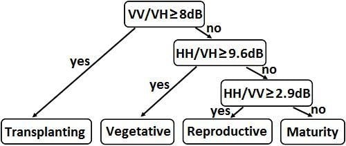
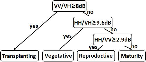
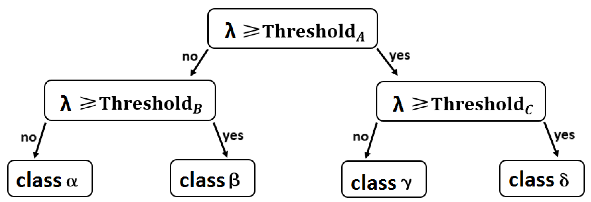
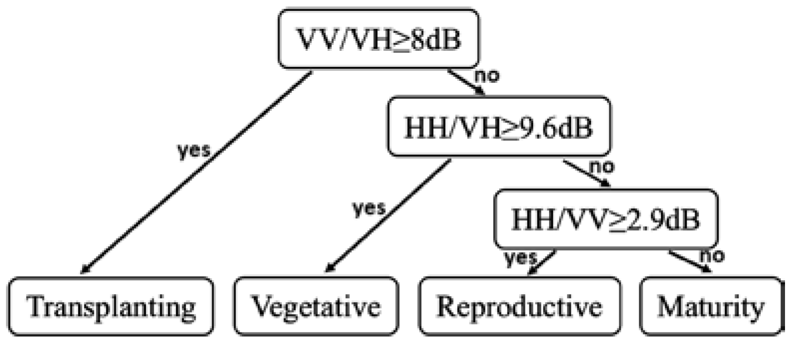
2.4. Decision Tree Method for Phenology Retrieval

The decision tree method is a classification strategy to process non-linear relationships between features and classes without any assumptions about the data probability distributions and to handle data measured on different scales [40]. The decision tree or similar methods like the decision plane is effective in rice monitoring with compact polarimetric (CP) parameters or target decomposition parameters [5,6,9]. The decision tree is of a treelike structure. The leaves are class labels, and intermediate nodes are criteria with several possible outcome branches. The classification processes begin at the root note and intermediate notes until encountering a leaf. A typical binary decision tree is shown in Figure 5.

In this study, four concerned phenological phases (i.e., transplanting, vegetative, reproductive, and maturity) need to be separated. Therefore, at least three thresholds are required. In order to distinguish rice phenology with the thresholds, one needs to ensure that backscattering coefficients or their combinations must have reliable separability among four critical phases. Since rice plants develop rapidly during the growing season and biophysical variables vary with phenological phases, the development phases are separable from each other. For example, distributions of the phases vs. VH backscattering coefficients are shown in Figure 6 using a boxplot. A division line near −20 dB can divide the transplanting phase from the other three. Similar division lines between other phenological phases were also observed on other polarizations (as shown in Figure 7). Once segmental thresholds to delineate four phenological phases were determined, a decision tree classifier could be developed to separate each development phase using backscattering coefficients.

3. Results

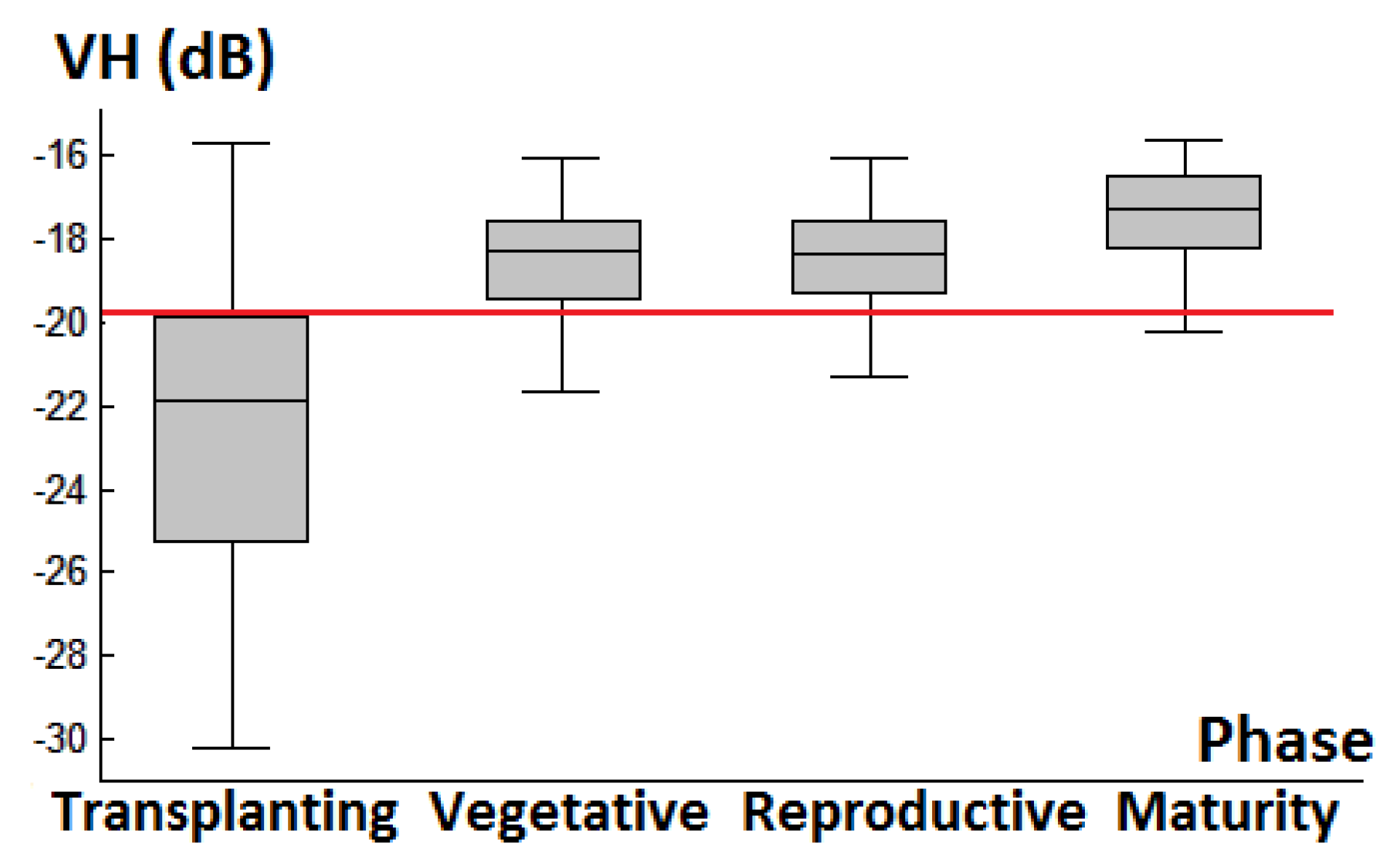
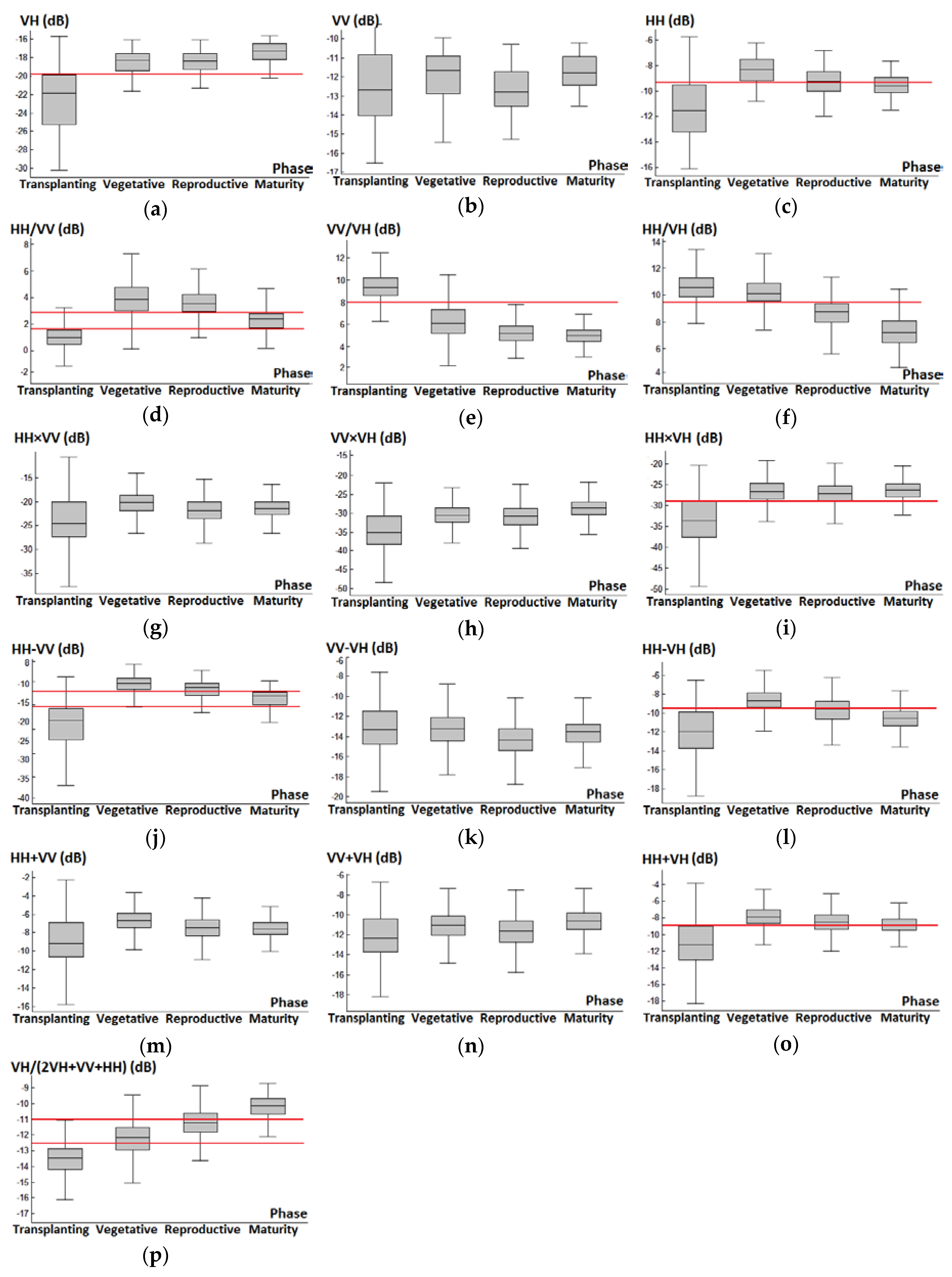
3.1. Backscattering Coefficient Analysis and Decision Tree Development

Distributions of backscattering coefficients of the training dataset, expressed in a logarithmic scale, and their combinations (calculated in linear scale then expressed in logarithmic scale) at each phase, are shown in boxplots (Figure 7). In the figure, VH/(2VH+VV+HH) was also plotted because of its sensitivity to vegetation parameters [41]. In each subplot, four boxes were drawn to represent the distributions of four phases. The red line visually showed a feasible division value. For example, the VH backscattering coefficients increased in general from the transplanting phase to the maturity phase (Figure 7a). The red line near −20 dB divided the transplanting phase from later phases with few data points crossing the division line. Ranges of the later phases, especially the vegetative and reproductive phase, severely overlapped with each other. Thus, VH data could not discriminate the vegetative phase from the reproductive phase.

As shown in Figure 7, there are varying degrees of overlaps between different phases and for different polarization data. The single polarized HH or VV data can hardly differentiate all phenological phases, but the joint use of several polarized data can achieve the needed separation. Taking subplot (d), (e), and (f) of Figure 7 as an example, one can use HH/VV data to divide the maturity phase from the vegetative and reproductive phases or the transplanting phase from the other three phases. The VV/VH parameter can be used to distinguish the transplanting phase from later phases. The HH/VH parameter can be used to differentiate the transplanting and vegetative phase from the reproductive and maturity phase. Thus, a combination of three polarized data can be used to distinguish four phenological phases. Then, a decision tree can be constructed (Figure 8).

Thresholds, 8 dB of VV/VH, 9.6 dB of HH/VH, and 2.9 dB of HH/VV, are optimal division lines which can separate the phases with the fewest overlaps of backscattering coefficient data (Figure 7). For instance, when a VV/VH threshold is set to 8 dB to divide the transplanting phase from the next three phases, the majority of backscattering coefficients are properly divided, and only 10.8% of backscattering coefficients overstep the threshold boundary, as shown in

Table 3. Thresholds of selected parameters. T stands for transplanting phase, V vegetative phase, R reproductive phase, and M maturity phase. An error rate means the proportion of pixels whose backscattering coefficients cross the threshold line.

	Decision Tree Parameters
	VV/VH	HH/VH	HH/VV
Divided Phase	T vs. V, R, or M	V vs. R or M	R vs. M
Threshold	8 dB	9.6 dB	2.9 dB
Error rate	10.8%	19.3%	23.2%

.

3.3. Validation

The performance of the decision tree classifier is tested using the reserved validation data. A confusion table [42] is built (

Table 4. Confusion table derived by validation data. UA stands for user's accuracy, PA producer's accuracy, and OA overall accuracy. Kappa denotes kappa coefficient.

		Ground Measured Phase
		Transplanting	Vegetative	Reproductive	Maturity	UA
Extracted phase	Transplanting	4	1	0	0	80%
	Vegetative	0	11	1	0	91.7%
	Reproductive	0	2	5	0	71.4%
	Maturity	0	0	0	5	100%
	PA	100%	78.6%	83.3%	100%	OA = 86.2%
						Kappa = 0.802

). The overall accuracy (OA) is 86.2%. The producer's accuracy (PA) is between 78.6% and 100%. The user's accuracy (UA) is between 71.4% and 100%. The kappa coefficient is 0.802.

The backscattering properties of a rice paddy during the transplanting period were mainly affected by water since the plant was small and the plan coverage was sparse. Thus, backscattering at this phase was quite different from that during the later three phases. As a result, backscattering coefficients of the transplanting phase were more distinctive by many polarized data (Figure 7). This was attributed to the high level of the determination accuracy (table 4). On the other hand, most of the misclassification occurred in the vegetative and reproductive phases because the water was very shallow or the field was dry. The rice canopy almost covered the fields continuously. Backscattering coefficients exhibited no distinctive changes from the vegetative phase to the reproductive phase for most polarized data (Figure 7). This was especially true during days of phase transition in which the plant height and water content of the plants changed slowly. The backscattering was mainly influenced by the plant density because rice plants in some fields had similar growth statuses (e.g., the number, size, orientation and water content of stems, leaves and young heads). The statuses usually differed because of different rice varieties and plants health.

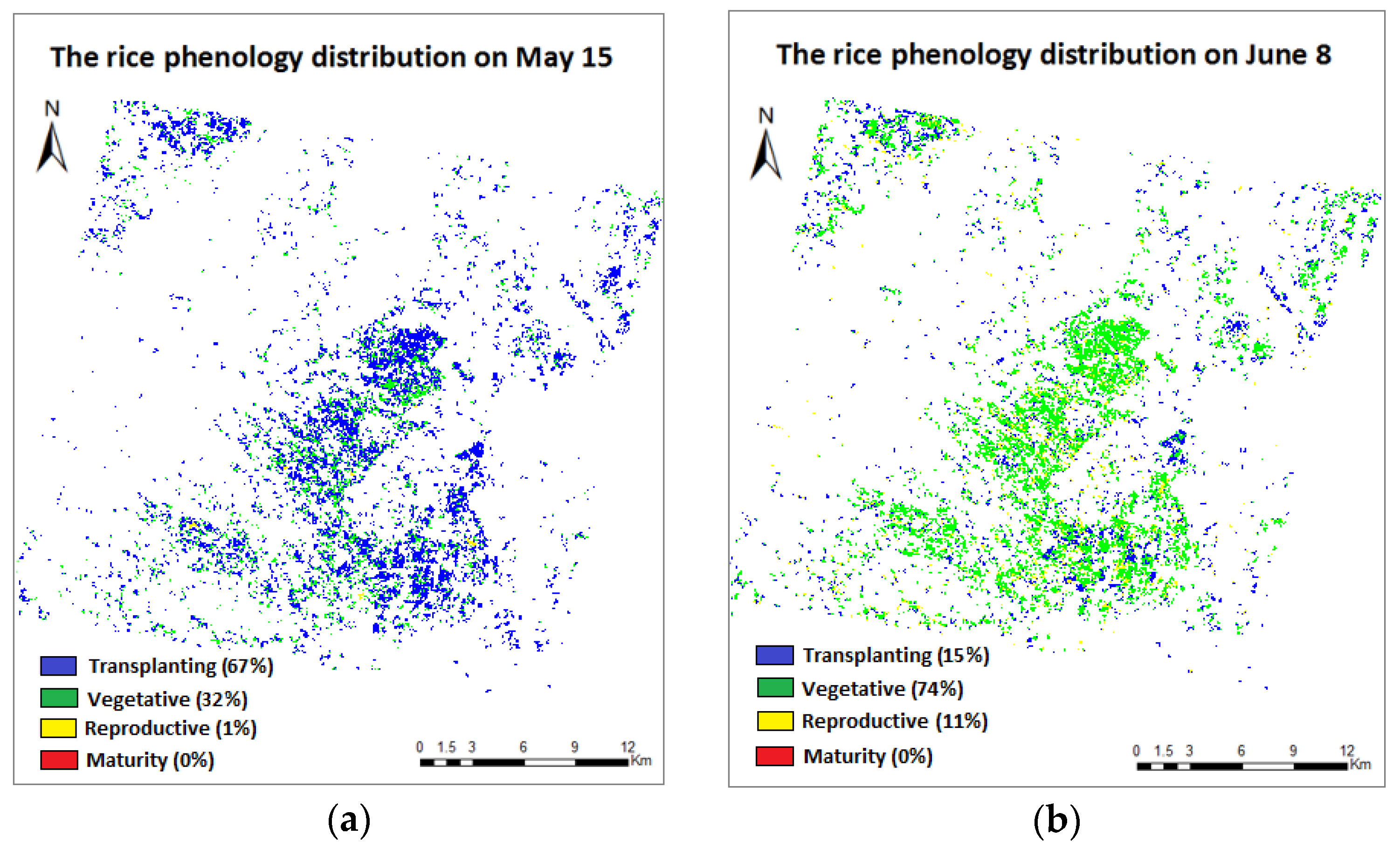
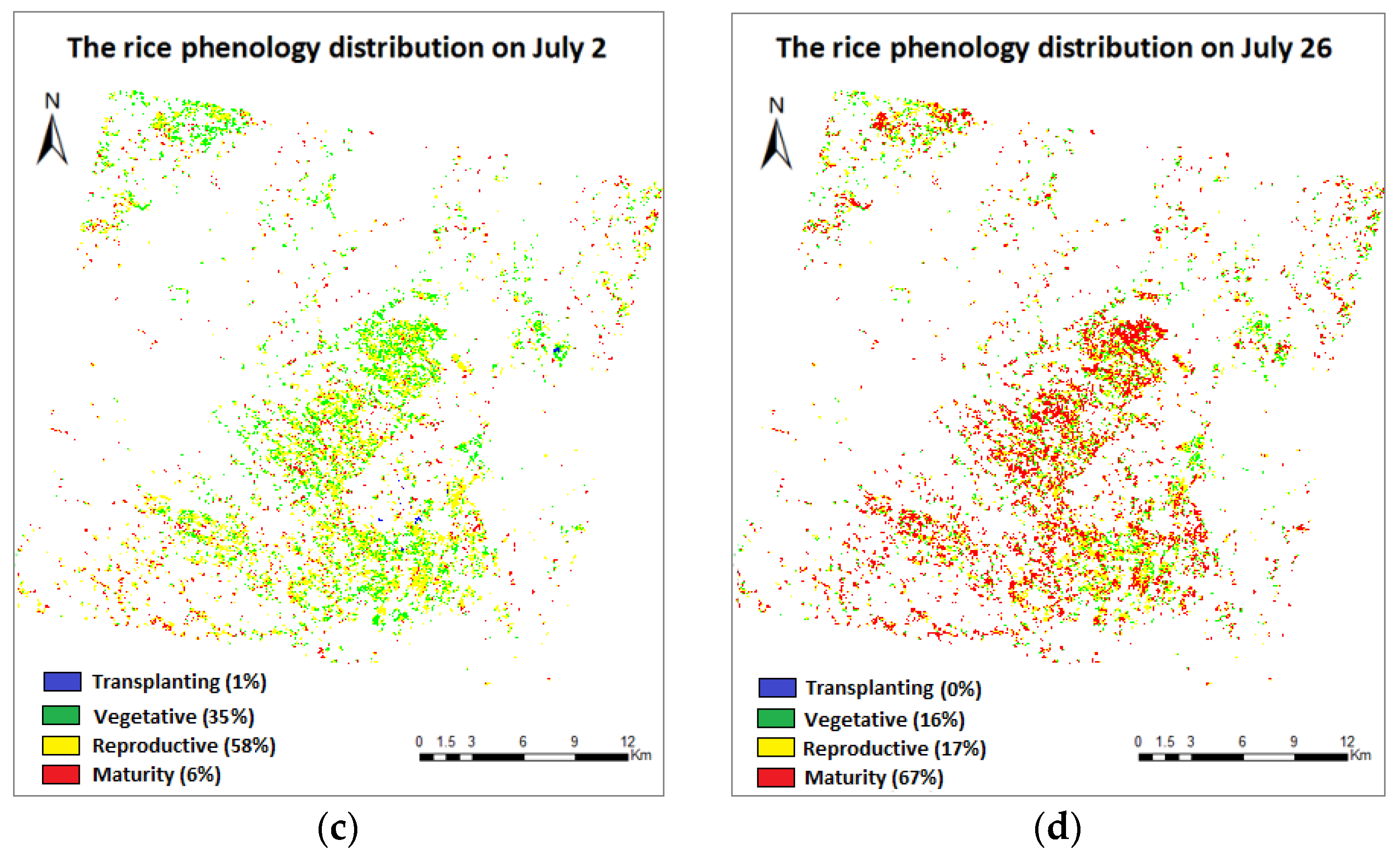
3.4. Phenology Extraction and Mapping

Based on the decision tree constructed in Figure 8, spatial distributions of rice phenology were mapped with multi-temporal SAR images (Figure 9). Pixels for the phase of transplanting, vegetative, reproductive, and maturity were colored blue, green, yellow, and red, respectively. Pixel statistics of each phase were annotated behind the legends, indicating a significant growth trend of rice paddies.

It is obvious that the spatial distribution of rice phenological phases varies on four dates, which shows a general trend of phenology evolution over time. On 15 May, almost all of the pixels are labeled as transplanting and vegetative phases, and transplanting pixels account for nearly 67%, showing that in most fields at this time, rice seedlings were just transplanted to the water and some earlier transplanted rice plants entered the vegetative phase. On 8 June, vegetative plants continued with the vegetative growth and prepared for the coming reproductive phase. Late seedlings were also extensively vegetative. These can be seen in map (b), where the pixels of the vegetative phase increase to an overwhelming proportion of 74%, while the transplanting ones sharply fall to 15%. On 2 July, about 58% of rice plants were in the reproductive phase. This ratio dropped to 17% on 26 July. In the last period, harvest pixels became the majority, with a proportion of 67%. All of these statistics are consistent with field survey observations, which demonstrates a feasibility of the decision tree classification.

4. Discussion

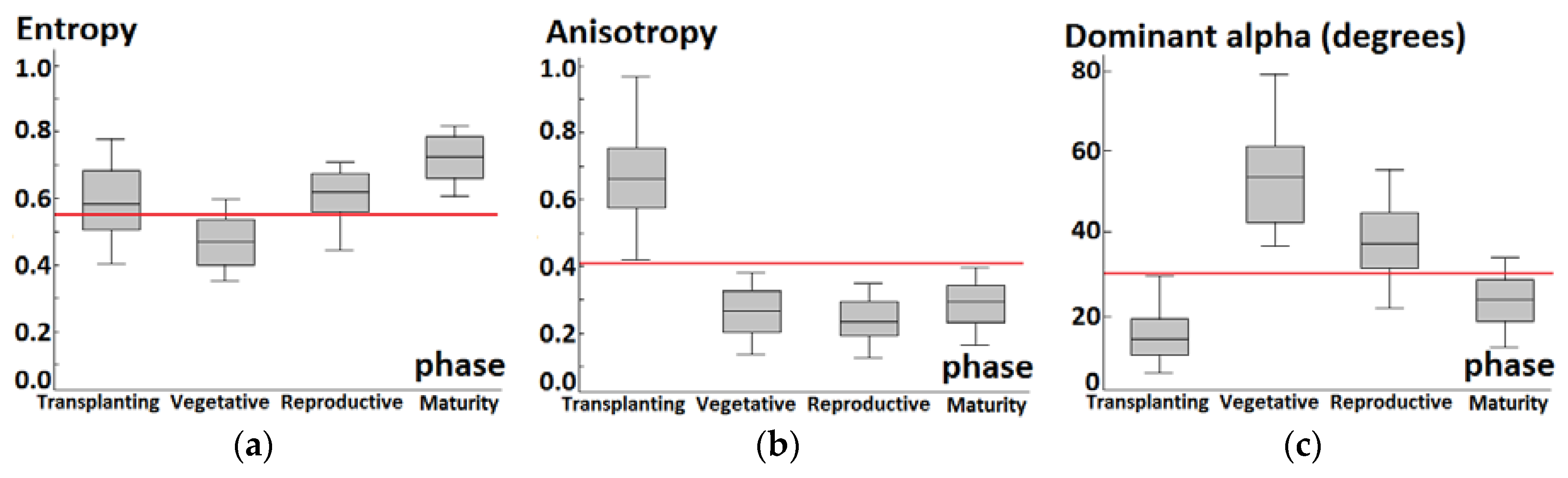
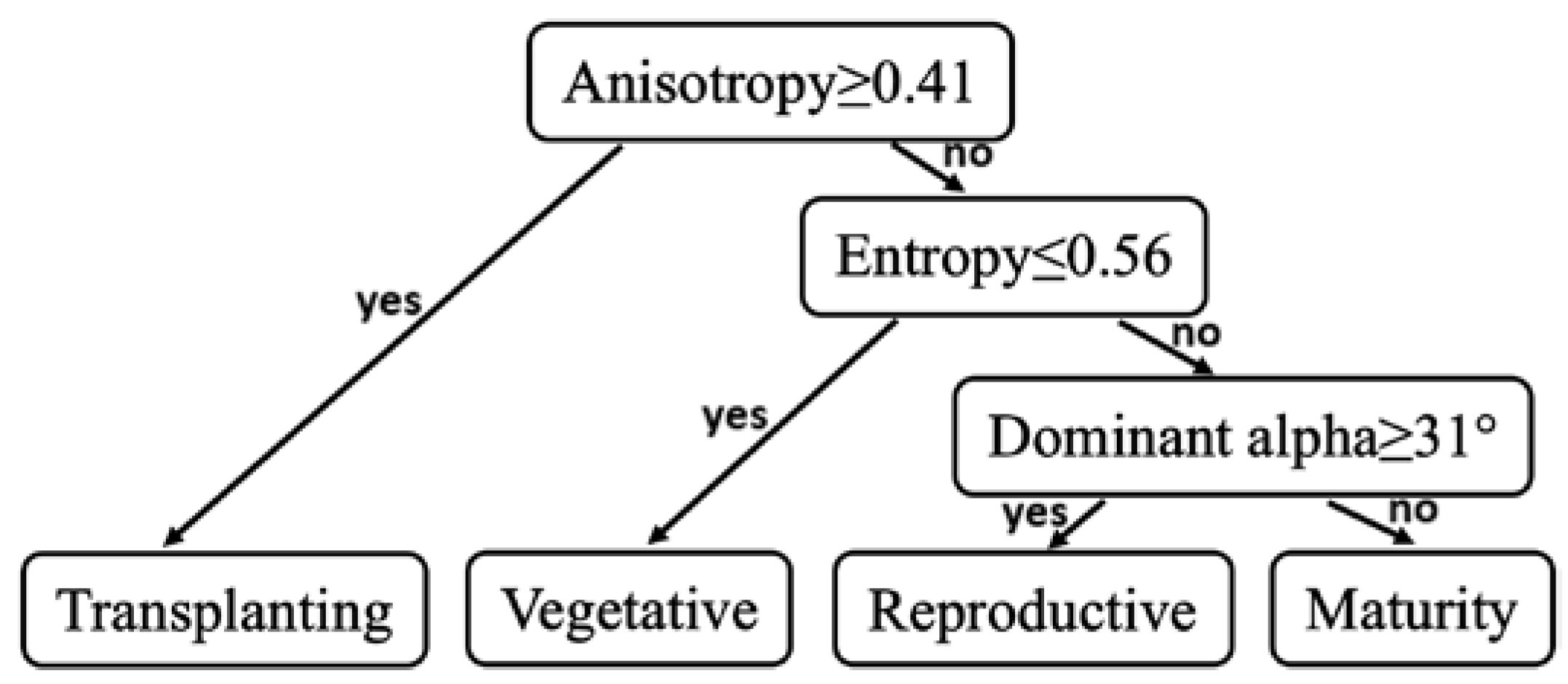
4.1. Phenology Extraction Comparison between Backscattering Coefficients and Decomposition Parameters

Compared with the most satisfactory retrieval accuracy given by previous studies, that is, Lopez-Sanchez et al. [6] used eigenvalue/vector decomposition parameters (entropy, anisotropy, and dominant alpha (${\mathsf{\alpha }}_1$, alpha of the dominant scattering mechanism)) to achieve an overall success rate of 96%, our study achieved a lower overall accuracy of 86.2%. In order to investigate the retrieval accuracy of the method proposed by Lopez-Sanchez et al. [6] in this study area, three eigenvalue/vector decomposition parameters (entropy, anisotropy, and dominant alpha) were extracted using the Polarimetric SAR Data Processing and Educational Tool (PolSARpro) software (http://step.esa.int/main/download/). The entropy (H) characterizes the randomness of the scattering processes. The anisotropy (A) characterizes the relative strengths of the second and third scattering mechanisms. The alpha angle (α) defines the scattering mechanism for a given eigenvector [43,44]. Dominant alpha (${\mathsf{\alpha }}_1$) is the alpha of the dominant scattering mechanism [6].

For each extracted decomposition parameter, we used all pixels of a sample site for averaging. Again, all decomposition parameters were divided into four groups based on phenological phases identified in field observations (i.e., transplanting, vegetative, reproductive, and maturity). Three-quarters of each group were chosen for training. The rest in each group were used for validation, respectively. Distributions of decomposition parameters (training dataset) during each phenological phase are shown in the boxplots of Figure 10.

A decision tree can be constructed using entropy, anisotropy, and dominant alpha (Figure 11), which is similar to the phenology retrieval algorithm designed by Lopez-Sanchez et al. [6].

The performance of the decision tree classifier is tested using the reserved validation data. A confusion table [42] is built (

Table 5. Confusion table derived by validation data for the phenology retrieval algorithm using entropy, anisotropy, and dominant alpha. UA stands for user's accuracy, PA producer's accuracy, and OA overall accuracy. Kappa denotes kappa coefficient.

		Ground Measured Phase
		Transplanting	Vegetative	Reproductive	Maturity	UA
Extracted hase	Transplanting	4	0	0	0	100%
	Vegetative	0	13	1	0	92.8 %
	Reproductive	0	1	5	0	83.3%
	Maturity	0	0	0	5	100%
	PA	100%	92.8%	83.3%	100%	OA = 93.1%
						Kappa = 0.89

).

The method using eigenvalue/vector decomposition parameters achieved a higher overall accuracy (93.1%) than the method using backscattering coefficients (86.2%). Compared with the backscattering coefficients method, the decomposition parameters method had two fewer wrong estimates (Tables 4 and 5). The first case corresponded to #8 sample site on 8 June. The phenology identified in the ground observation was stage 32 (vegetative phase), but the backscattering coefficients method misclassified the rice plants at the transplanting phase. Plants at #8 sample site were the last to enter the transplanted phase. On 8 June, tillers and leaves were only partially developed, which resulted in relatively low VH backscattering coefficients (about −20 dB). Scattering from the rough surface of the flooded ground made VV exhibit a relatively high value (about −12 dB). Thus, rice plants at #8 sample site had similar VV/VH values with the transplanting ones. However, using decomposition parameters can correctly determine the phenology because low anisotropy (about 0.32) was observed due to the comparable contribution from surface scattering and double-bounce scattering, which were weaker than volume scattering during this time. The second case corresponded to #24 sample site on 2 July. The ground campaign indicated that the rice plants were in stage 44 (vegetative phase), whereas the backscattering coefficients method misclassified their phase as the reproductive phase. One possible cause for the misclassification was that rice at the #24 sample site had a denser canopy than other sites on 2 July. The attenuation by the denser canopy resulted in lower HH backscattering coefficients. Hence rice plants at the #24 sample site had similar HH/VH values with the plants in reproductive phase. However, the low entropy (about 0.5) of the #24 sample site can be used to identify the vegetative phase. Since the ears had not appeared and the stems were mostly vertical, double-bounce scattering still contributed significantly to the radar backscattering mechanism. Another two wrong estimates of the backscattering coefficients method also appeared in the decomposition parameters method. Corresponding rice plants were in the transition period from the vegetative to the reproductive phase (stage 47 and 55). The gradual change of rice plants and the similar backscatter properties of fields during this period caused the misclassification.

In general, the phenology retrieval method using backscattering coefficients is less effective than the method using eigenvalue/vector decomposition parameters. Since additional data (phase data) are considered in the decomposition, eigenvalue/vector decomposition parameters can provide more information on the physical scattering mechanism. However, the result of the backscattering coefficients method is still acceptable because only amplitude information of backscattering coefficients is used.

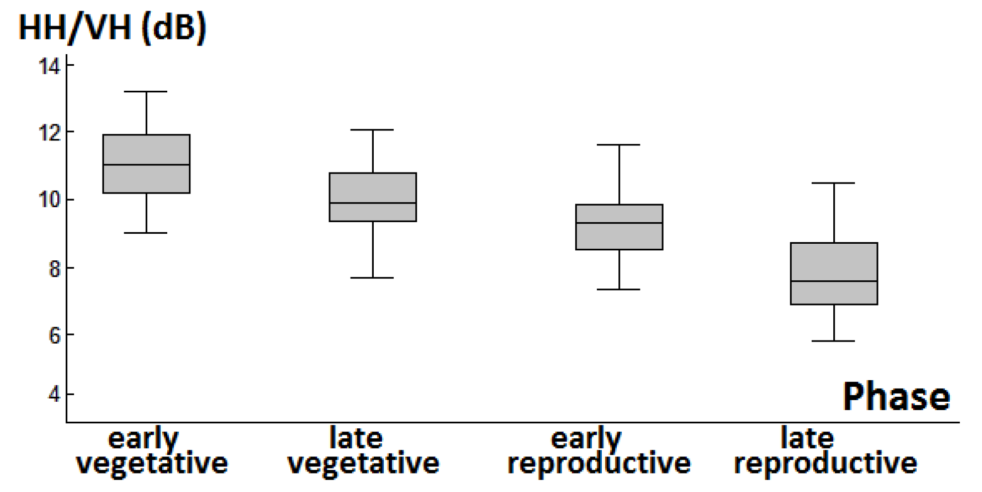
4.2. Response of Backscattering Coefficients in Phenology Retrieval

Evolution of the backscattering coefficients during the growing season (Figure 7) reflected the characteristics of rice phenology evolution and growth status change. By taking advantage of responses of backscattering coefficients to different polarizations and in different phenological phases, the phenology retrieval method (Figure 8) achieved a high overall accuracy (86.2%).

During the transplanting phase, rice plants were very small and short. The amount of scattering attenuation was small because of the low rice height and sparse rice canopy. The Bragg scattering from the rough surface of the flooded ground predicted that VV backscattering coefficients had moderate values (−12.5 dB on average) [5,26]. VH backscattering coefficients were low (−22 dB on average) because of the sparse rice canopy since VH polarization was sensitive to volume scattering from the rice canopy [25,26]. HH backscattering coefficients were low (compared with later phases) due to the weak double-bounce scattering between the small rice plants and the underlying water surface, since HH polarization was sensitive to double-bounce scattering between rice plants and the ground surface [45]. The difference between the responses at VV and VH was clearly illustrated by the VV/VH ratio, which can be used to separate the transplanting phase from later phases.

During the vegetative phase, VH increased significantly with the development of the plants and hence with increasing canopy density. HH also increased significantly because of the larger stalks and increasing plants height. Double-bounce scattering between the rice plants and the underlying surface increased [26]. VV increased slightly because it was affected by an extinction due to the vertical preferred orientation of the plant elements (e.g., stems and leaves) [6].

During the reproductive phase, VH increased due to the denser plants canopy. Rice heads emerged as new scattering elements in the upper part of the canopy. HH decreased because the dense canopy reduced the microwave penetration to the surface and the double bounce off the rice plants [29]. VV decreased because the stems remained predominantly vertical and the amount of double-bounce and surface scattering was small [26]. Because of the different trends in the HH and VH channels, the HH/VH ratio can be used to separate the vegetative phase from later phases.

During the maturity phase, VH increased because the amount and size of rice heads increased. HH decreased because of the large amount of attenuation by the rice canopy and the low volumetric moisture content. Stems became drier and the reduced water content caused less vertical extinction, especially for VV polarization [25]. The orientation of plant elements (i.e., stems, leaves, and heads) became random during this period. The attenuation of the VV polarization by the vertical orientation of the cylinders was reduced [25]. Therefore, VV stopped decreasing and the HH/VV ratio can be used to separate the reproductive phase from the maturity phase due to the different trends in HH and VV channels.

Most of the misclassification occurred in the transition from the vegetative to the reproductive phase, as shown in Table 4. In this period, backscattering properties of rice plants were mainly influenced by planting density and rice plants growth status, which were usually affected by rice varieties and plants health. Late vegetative (from stage 40 to 49) rice plants had similar backscatter properties with early reproductive (from stage 50 to 59) rice plants because of the gradual development of plants morphological structure. As shown in Figure 12, values of HH/VH decreased monotonously from the early vegetative phase (from stage 20 to 39) to the late reproductive phase (from stage 60 to 69). The slow growth of rice plants and weak rice heads at the turn of the vegetative and reproductive phase resulted in no significant change of HH/VH data. Range overlap appeared during the late vegetative and early reproductive phase. As the water content of rice plants continuously fell and rice heads gradually became important scattering elements in the late reproductive phase, backscatter properties exhibited a notable change.

There are still several issues waiting to be addressed in further research and development. First, since phenology evolution is a continuous process, dividing phenology into discrete intervals makes it hard to decide whether the plants are in one phase or another during the transition between phases. For example, ground observation indicated that rice plants at #19 sample site on 2 July were at the vegetative phase (stage 47), whereas the retrieval algorithm misclassified them as reproductive plants (stages 50–69). In the BBCH scale, an error between stage 47 and 50 is minimal (3 over 100), but in discrete intervals, it means an error between two phases (1 over 4). A possible alternative to avoid this problem consists of dividing phenology into more phases or retrieving phenology in a continuous range. This brings up another issue, that is, more ground observation and SAR data are needed. Rice plants grow rapidly during the bimestrial season. The phenological phase (e.g., transplanting and reproductive phase) lasts about two weeks on average and phase transition usually takes place in a short interval. The 24-day revisit period of RADARSAT-2 is relatively long for monitoring growth changes timely. To overcome this problem, different spaceborne C-band SAR sensors (e.g., Sentinel-1 and Gaofen-3) can be combined to increase the temporal resolution of SAR observations.

5. Conclusions

We analyzed statistical relationships between backscatter coefficients and rice phenology using multi-temporal quad-polarized RADARSAT-2 SAR datasets and rice biophysical data measured in the Meishan study area, Sichuan Province, China. Although the degree of the correlation is affected by uncertain factors such as diverse patterns of rice cultivation, there was a strong correlation between the RADARSAT-2 backscattering coefficients and rice phenology.

VH, VV, and HH backscattering coefficients were used to distinguish transplanting, vegetative, reproductive, and maturity phases. In particular, the VV/VH threshold was used to separate plants in the transplanting phase from plants in the vegetative, reproductive, and maturity phases, the HH/VH threshold to delineate plants in the vegetative phase from plants in the reproductive and maturity phases, and the HH/VV threshold to distinguish plants in the reproductive phase from plants in the maturity phase. Then, a decision tree classifier was developed. The accuracy level was 86.2% in the delineation of rice phenology. The analysis procedure was relatively simple, ensuring the reliability of the method. Therefore, there should be a great potential to use RADARSAT-2 SAR data to monitor rice phenology during its growth period and in large spatial extent. Finally, the concise decision logic should make this study easy understood and implemented in other studies related to local rice production.

References

1. Chen, C.; Son, N.T.; Chang, L. Monitoring of rice cropping intensity in the upper Mekong Delta, Vietnam using time-series MODIS data. Adv. Space Res. 2012, 49, 292–301. [Google Scholar] [CrossRef]
2. McLean, J.; Hardy, B.; Hettel, G. Rice Almanac, 4th ed.; International Rice Research Institute: Los Banos, Philippines, 2013; ISBN 978-971-22-0300-8. [Google Scholar]
3. Sakamoto, T. A crop phenology detection method using time-series MODIS data. Remote Sens. Environ. 2005, 96, 366–374. [Google Scholar] [CrossRef]
4. Lausch, A.; Salbach, C.; Schmidt, A.; Doktor, D.; Merbach, I.; Pause, M. Deriving phenology of barley with imaging hyperspectral remote sensing. Ecol. Model. 2015, 295, 123–135. [Google Scholar] [CrossRef]
5. Lopez-Sanchez, J.M.; Cloude, S.R.; Ballester-Berman, J.D. Rice phenology monitoring by means of SAR polarimetry at X-band. IEEE Trans. Geosci. Remote Sens. 2012, 50, 2695–2709. [Google Scholar] [CrossRef]
6. Lopez-Sanchez, J.M.; Vicente-Guijalba, F.; Ballester-Berman, J.D.; Cloude, S.R. Polarimetric response of rice fields at C-band: Analysis and phenology retrieval. IEEE Trans. Geosci. Remote Sens. 2014, 52, 2977–2993. [Google Scholar] [CrossRef]
7. Vicente-Guijalba, F.; Martinez-Marin, T.; Lopez-Sanchez, J.M. Crop phenology estimation using a multitemporal model and a Kalman filtering strategy. IEEE Geosci. Remote Sens. Lett. 2014, 11, 1081–1085. [Google Scholar] [CrossRef]
8. Xu, D.; Fu, M. Detection and modeling of vegetation phenology spatiotemporal characteristics in the middle part of the Huai river region in China. Sustainability 2015, 7, 2841–2857. [Google Scholar] [CrossRef]
9. Yang, Z.; Li, K.; Liu, L.; Shao, Y.; Brisco, B.; Li, W. Rice growth monitoring using simulated compact polarimetric C band SAR. Radio Sci. 2014, 49, 1300–1315. [Google Scholar] [CrossRef]
10. Zhang, Y.; Li, L.; Wang, H.; Zhang, Y.; Wang, N.; Chen, J. Land surface phenology of Northeast China during 2000-2015: temporal changes and relationships with climate changes. Environ Monit Assess. 2017, 189. [Google Scholar] [CrossRef] [PubMed]
11. Li, S.; Xiao, J.; Ni, P.; Zhang, J.; Wang, H.; Wang, J. Monitoring paddy rice phenology using time series MODIS data over Jiangxi Province, China. Int. J. Agric. & Biol. Eng. 2014, 7, 28–36. [Google Scholar]
12. Dash, J.; Jeganathan, C.; Atkinson, P.M. The use of MERIS Terrestrial Chlorophyll Index to study spatio-temporal variation in vegetation phenology over India. Remote Sens. Environ. 2010, 114, 1388–1402. [Google Scholar] [CrossRef]
13. Corcione, V.; Nunziata, F.; Mascolo, L.; Migliaccio, M. A study of the use of COSMO-SkyMed SAR PingPong polarimetric mode for rice growth monitoring. Int. J. Remote Sens. 2016, 37, 633–647. [Google Scholar] [CrossRef]
14. Peng, D.; Huete, A.R.; Huang, J.; Wang, F.; Sun, H. Detection and estimation of mixed paddy rice cropping patterns with MODIS data. Int. J. Appl. Earth Obs. Geoinf. 2011, 13, 13–23. [Google Scholar] [CrossRef]
15. Motohka, T.; Nasahara, K.N.; Miyata, A.; Mano, M.; Tsuchida, S. Evaluation of optical satellite remote sensing for rice paddy phenology in monsoon Asia using a continuous in situ dataset. Int. J. Remote Sens. 2009, 30, 4343–4357. [Google Scholar] [CrossRef]
16. Boschetti, L.; Roy, D.P. Strategies for the fusion of satellite fire radiative power with burned area data for fire radiative energy derivation. J. Geophys. Res. Atmos. 2009, 114, 215–216. [Google Scholar] [CrossRef]
17. Wang, H.; Chen, J.; Wu, Z.; Lin, H. Rice heading date retrieval based on multi-temporal MODIS data and polynomial fitting. Int. J. Remote Sens. 2012, 33, 1905–1916. [Google Scholar] [CrossRef]
18. Wang, J.; Huang, J.; Wang, X.; Jin, M.; Zhou, Z.; Guo, Q.; Zhao, Z.; Huang, W.; Zhang, Y.; Song, X. Estimation of rice phenology date using integrated HJ-1 CCD and Landsat-8 OLI vegetation indices time-series images. J. Zhejiang Univ. Sci. B 2015, 16, 832–844. [Google Scholar] [CrossRef] [PubMed]
19. Zhang, Y.; Liu, X.; Su, S.; Wang, C. Retrieving canopy height and density of paddy rice from Radarsat-2 images with a canopy scattering model. Int. J. Appl. Earth Obs. Geoinf. 2014, 28, 170–180. [Google Scholar] [CrossRef]
20. Bouvet, A.; Le Toan, T.; Lam-Dao, N. Monitoring of the rice cropping system in the Mekong delta using ENVISAT/ASAR dual polarization data. IEEE Trans. Geosci. Remote Sens. 2009, 47, 517–526. [Google Scholar] [CrossRef] [Green Version]
21. Yuzugullu, O.; Erten, E.; Hajnsek, I. Rice Growth monitoring by means of X-Band co-polar SAR: Feature clustering and BBCH scale. IEEE Geosci. Remote Sens. Lett. 2015, 12, 1218–1222. [Google Scholar] [CrossRef]
22. Ҫağlar, K.; Gülşen, T.; Erten, E. Paddy-rice phenology classification based on machine-learning methods using multi-temporal co-polar X-Band SAR images. IEEE J. Sel. Top. Appl. Earth Observ. Remote Sens. 2016, 9, 2509–2519. [Google Scholar]
23. De Bernardis, C.G.; Vicente-Guijalba, F.; Martinez-Marin, T.; Lopez-Sanchez, J.M. Estimation of key dates and stages in rice crops using dual-polarization SAR time series and a particle filtering approach. IEEE J. Sel. Top. Appl. Earth Observ. Remote Sens. 2015, 8, 1008–1018. [Google Scholar] [CrossRef]
24. Erten, E.; Lopez-Sanchez, J.M.; Yuzugullu, O.; Hajnsek, I. Retrieval of agricultural crop height from space: A comparison of SAR techniques. Remote Sens. Environ. 2017, 187, 130–144. [Google Scholar] [CrossRef]
25. Koppe, W.; Gnyp, M.L.; Hütt, C.; Yao, Y.; Miao, Y.; Chen, X.; Bareth, G. Rice monitoring with multi-temporal and dual-polarimetric TerraSAR-X data. Int. J. Appl. Earth Obs. Geoinf. 2013, 21, 568–576. [Google Scholar] [CrossRef]
26. Yang, Z.; Shao, Y.; Li, K.; Liu, Q.; Liu, L.; Brian, B. An improved scheme for rice phenology estimation based on time-series multispectral HJ-1A/B and polarimetric RADARSAT-2 data. Remote Sens. Environ. 2017, 195, 184–201. [Google Scholar] [CrossRef]
27. Francis, C.; Shang, J.; Liu, J.; Huang, X.; Ma, B.; Jiao, X.; Geng, X.; John, M.K.; Dan, W. Tracking crop phenological development using multi-temporal polarimetric Radarsat-2 data. Remote Sens. Environ. 2017. [Google Scholar] [CrossRef]
28. Tian, H.; Wu, M.; Wang, L.; Niu, Z. Mapping early, middle and late rice extent using sentinel-1A and Landsat-8 data in the poyang lake plain, China. Sensors 2018, 18, 185. [Google Scholar] [CrossRef] [PubMed]
29. Inoue, Y.; Kurosu, T.; Maeno, H.; Uratsuka, S.; Kozu, T.; Dabrowska-Zielinska, K.; Qi, J. Season-long daily measurements of multifrequency (Ka, Ku, X, C, and L) and full-polarization backscatter signatures over paddy rice field and their relationship with biological variables. Remote Sens. Environ. 2002, 81, 194–204. [Google Scholar] [CrossRef]
30. Wu, F.; Wang, C.; Zhang, H.; Zhang, B.; Tang, Y. Rice crop monitoring in South China with RADARSAT-2 quad-polarization SAR data. IEEE Geosci. Remote Sens. Lett. 2011, 8, 196–200. [Google Scholar] [CrossRef]
31. Li, S.; Ni, P.; Cui, G.; He, P.; Liu, H.; Li, L.; Liang, Z. Estimation of rice biophysical parameters using multitemporal RADARSAT-2 images. In Proceedings of the Symposium of the International Society for Digital Earth (ISDE), Halifax, NS, Canada, 5–9 October 2015; p. 012019. [Google Scholar]
32. Yang, S.; Zhao, X.; Li, B.; Hua, G. Interpreting RADARSAT-2 quad-polarization SAR signatures from rice paddy based on experiments. IEEE Geosci. Remote Sens. Lett. 2012, 9, 65–69. [Google Scholar] [CrossRef]
33. Ulaby, F.; Allen, C.; Eger, G.; Kanemasu, E. Relating the microwave backscattering coefficient to leaf area index. Remote Sens. Environ. 1984, 14, 113–133. [Google Scholar] [CrossRef]
34. Bouman, B. Crop parameter estimation from ground-based X-band (3-cm wave) radar backscattering data. Remote Sens. Environ. 1991, 37, 193–205. [Google Scholar] [CrossRef]
35. Inoue, Y.; Sakaiya, E. Relationship between X-band backscattering coefficients from high-resolution satellite SAR and biophysical variables in paddy rice. Remote Sens. Lett. 2013, 4, 288–295. [Google Scholar] [CrossRef]
36. Inoue, Y.; Sakaiya, E.; Wang, C. Capability of C-band backscattering coefficients from high-resolution satellite SAR sensors to assess biophysical variables in paddy rice. Remote Sens. Environ. 2014, 140, 257–266. [Google Scholar] [CrossRef]
37. Yuzugullu, O.; Erten, E.; Hajnsek, I. Estimation of rice crop height from X- and C-Band PolSAR by Metamodel-Based optimization. IEEE J. Sel. Top. Appl. Earth Observ. Remote Sens. 2017, 10, 194–204. [Google Scholar] [CrossRef]
38. Zadoks, J.C.; Chang, T.T.; Konzak, C.F. A decimal code for the growth stages of cereals. Weed Res. 1974, 14, 415–421. [Google Scholar] [CrossRef]
39. Rossi, C.; Erten, E. Paddy-rice monitoring using TanDEM-X. IEEE Trans. Geosci. Remote Sens. 2015, 53, 900–910. [Google Scholar] [CrossRef]
40. Pal, M.; Mather, P.M. An assessment of the effectiveness of decision tree methods for land cover classification. Remote Sens. Environ. 2003, 86, 554–565. [Google Scholar] [CrossRef]
41. Francis, C.; Richard, F. ALOS PALSAR L-band polarimetric SAR data and in situ measurements for leaf area index assessment. Remote Sens. Lett. 2012, 3, 221–229. [Google Scholar]
42. Congalton, R.G. Accuracy assessment and validation of remotely sensed and other spatial information. Int. J. Wildland Fire. 2001, 10, 321–328. [Google Scholar] [CrossRef]
43. Cloude, S.R.; Pottier, E. An entropy based classification scheme for land applications of polarimetric SAR. IEEE Trans. Geosci. Remote Sens. 1997, 35, 68–78. [Google Scholar] [CrossRef]
44. Pacheco, A.; McNairn, H.; Li, Y.; Lampropoulos, G.; Powers, J. Using RADARSAT-2 and TerraSAR-X satellite data for the identification of canola crop phenology. SPIE Remote Sens. 2016, 9998. [Google Scholar] [CrossRef]
45. Wang, L.; Kong, J.; Ding, K.; Le Toan, T.; Ribbes-Baillarin, F.; Floury, N. Electromagetic scattering model for rice canopy based on Monte Carlo simulation. Prog. Electromagn. Res. 2005, 52, 153–171. [Google Scholar] [CrossRef]
Figure 1. The study area imaged by the French SPOT-6 optical sensor on 15 July 2016. Thirty sample sites are located and numbered.
Remotesensing 10 00340 g001
Figure 2. Four rice phenological phases in the study area in 2016. (a) transplanting, (b) vegetative, (c) reproductive, and (d) maturity.
Remotesensing 10 00340 g002
Figure 3. In situ rice phenology at 30 sample sites in 2016. Blue, green, yellow, and red dots, respectively, represent the transplanting, vegetative, reproductive, and maturity phase. Four horizontal lines denote the acquisition dates of four RADARSAT-2 datasets.
Remotesensing 10 00340 g003
Figure 4. A RADARSAT-2 image acquired on 2 July 2016. VH, VV, and HH bands were assigned as red, green, and blue colors, respectively. Study area is within the yellow box.
Remotesensing 10 00340 g004
Figure 5. A simple decision tree of a variable, λ. Three thresholds divide λ into four classes through two decision layers.
Remotesensing 10 00340 g005
Figure 6. Distributions of development phases vs. VH backscattering coefficients. The data are training data. At about −20 dB, the transplanting phase is separated from other three phases.
Remotesensing 10 00340 g006
Figure 7. Boxplots of backscattering coefficients (training dataset, expressed in logarithmic scale) and their combinations (calculated in linear scale then expressed in logarithmic scale) at each phase, (a) VH, (b) VV, (c) HH, (d) HH/VV, (e) VV/VH, (f) HH/VH, (g) HH × VV, (h) VV × VH, (i) HH × VH, (j) HH − VV, (k) VV − VH, (l) HH − VH, (m) HH + VV, (n) VV + VH, (o) HH + VH, (p) VH/(2VH + VV + HH). Red lines represent possible division values to separate at least two interquartile ranges (grey part of boxes).
Remotesensing 10 00340 g007
Figure 8. A decision tree classifier. Thresholds of VV/VH, HH/VV, and HH/VH divide SAR data into four phenological phases.
Remotesensing 10 00340 g008
Figure 9. Map of rice phenological phases spatial distribution on (a) 15 May, (b) 8 June, (c) 2 July, and (d) 26 July. Blue, green, yellow, and red colors, respectively, represent transplanting, vegetative, reproductive, and maturity phases of rice plants in the study area.
Remotesensing 10 00340 g009aRemotesensing 10 00340 g009b
Figure 10. Evolution of observables (training dataset) provided by the eigenvalue/vector decomposition of the coherency matrix versus phenology, (a) Entropy, (b) Anisotropy, (c) Dominant alpha angle ( α 1 , alpha of the dominant scattering mechanism). Red lines represent possible division values to separate at least two interquartile ranges (grey part of boxes).
Remotesensing 10 00340 g010
Figure 11. Phenology decision tree. Thresholds of anisotropy, entropy, and dominant alpha angle divide SAR data into four phenological phases.
Remotesensing 10 00340 g011
Figure 12. Gradual temporal change of HH/VH data on subdivisions of vegetative and reproductive phase.
Remotesensing 10 00340 g012