Development of a System of Compatible Individual Tree Diameter and Aboveground Biomass Prediction Models Using Error-In-Variable Regression and Airborne LiDAR Data

Abstract

Estimating individual tree diameters at breast height (DBH) from delineated crowns and tree heights on the basis of airborne light detection and ranging (LiDAR) data provides a good opportunity for large-scale forest inventory. Generally, ground-based measurements are more accurate, but LiDAR data and derived DBH values can be obtained over larger areas for a relatively smaller cost if a right procedure is developed. A nonlinear least squares (NLS) regression is not an appropriate approach to predict the aboveground biomass (AGB) of individual trees from the estimated DBH because both the response variable and the regressor are subject to measurement errors. In this study, a system of compatible individual tree DBH and AGB error-in-variable models was developed using error-in-variable regression techniques based on both airborne LiDAR and field-measured datasets of individual Picea crassifolia Kom. trees, collected in northwestern China. Two parameter estimation algorithms, i.e., the two-stage error-in-variable model (TSEM) and the nonlinear seemingly unrelated regression (NSUR), were proposed for estimating the parameters in the developed system of compatible individual tree DBH and AGB error-in-variable models. Moreover, two model structures were applied to estimate AGB for comparison purposes: NLS with AGB estimation depending on DBH (NLS&DD) and NLS with AGB estimation not depending on DBH (NLS&NDD). The results showed that both TSEM and NSUR led to almost the same parameter estimates for the developed system. Moreover, the developed system effectively accounted for the inherent correlation between DBH and AGB as well as for the effects of measurement errors in the DBH on the predictions of AGB, whereas NLS&DD and NLS&NDD did not. A leave-one-out cross-validation indicated that the prediction accuracy of the developed system of compatible individual tree DBH and AGB error-in-variable models with NSUR was the highest among those estimated by the four methods evaluated, but, statistically, the accuracy improvement was not significantly different from zero. The main reason might be that, except for the measurement errors, other source errors were ignored in the modeling. This study implies that, overall, the proposed method provides the potential to expand the estimations of both DBH and AGB from individual trees to stands by combining the error-in-variable modeling and LiDAR data and improve their estimation accuracies, but its application needs to be further validated by conducting a systematical uncertainty analysis of various source errors in a future study.

1. Introduction

The timely and cost-effective acquisition of forest inventory data, including forest carbon, at a large scale, has long been of concern for sustainable management and planning of forest ecosystems [1,2]. Tree diameter at breast height (DBH) and biomass are the two of the most common measures of tree size in forest mensuration. Moreover, tree DBH and biomass are also two essential factors in forest growth and yield modeling. Although tree DBH can be easily measured on the ground with high accuracy, ground measurements of tree biomass are less accurate and often difficult, time-consuming, and costly. Consequently, DBH is usually measured for all trees in ground-based forest inventories, experimental and permanent growth plots, but tree biomass measurements are usually obtained from an affordable number of sample trees [3]. Correspondingly, a large number of aboveground biomass-, belowground biomass-, and total biomass-DBH equations have been developed for numerous species in many forest types over the last 20 years [2,3,4,5,6,7,8]. As a result of these studies, predicting tree biomass from DBH has become a well-established technique, widely applied in forest inventory and growth and yield predictions. However, the collection of DBH data at a large scale can also be costly and time-consuming.

The affordability and capability of high spatial resolution images from airborne sensors and satellite systems have made it possible to accurately extract information of tree variables from the images at a large scale and then establish the relationship of a tree biomass with the tree variables that are measurable on the ground and can be also accurately estimated from the images [9,10,11,12,13,14]. Therefore, the methods for obtaining DBH have shifted from conventional ground-based forest inventories to modeling and prediction based on remote sensing technologies [11,15,16,17].

Light detection and ranging (LiDAR) is one of the most promising remote sensing technologies for estimating various biophysical properties of forests and has been widely applied in forest measurement and inventory over the past two decades [14,18]. The technique, implying the automatic extraction of information of individual trees instead of stands on the basis of LiDAR data, has drawn great attention in recent years [1,11,19]. LiDAR provides accurate estimates of terrain elevation and vegetation height, and this holds even on sloped terrain or in dense and complex forests [20]. The use of LiDAR data is appropriate to estimate tree DBH and biomass, as point clouds generated from forest canopies can accurately depict the physical characteristics of the canopy surface and structure [21]. The physical characteristics, including tree height, crown projection area, crown diameter and shape, are often significantly correlated with the tree DBH and biomass, and have been commonly utilized to develop their relationships with either DBH or biomass and further obtain LiDAR-derived tree variables-DBH or -biomass models [1,11,15,19].

In practice, a nonlinear least squares regression (NLS) has been used to estimate the parameters in the LiDAR-derived tree variables–DBH or –biomass models [1,11,22]. This method is generally acknowledged as a standard regression technique for modeling the relationship between variables. Its major assumptions are as follows: (i) the dependent variable is a random variable; (ii) the independent variables are fixed and observed without errors; (iii) the model error term has an independent and identical normal distribution with a zero mean and constant variance [23]. It is well known that the violation of the second assumption above may lead to biased estimates of the regression coefficients and/or of the standard errors of the coefficients and, consequently, to misleading hypothesis testing [23,24]. The non-normal distribution of the model error term may also mislead hypothesis testing even though the NLS coefficients and standard errors would be estimated without bias.

Although tree biomass may be estimated from LiDAR-derived tree height or crown attributes (such as crown width) alone, the accuracy of such estimates is often not satisfactory [25]. The estimated DBH from LiDAR–DBH models and the physical characteristics extracted from remote sensing images (e.g., LiDAR-derived tree height) have been commonly used to estimate tree biomass based on LiDAR-biomass models (e.g., allometric biomass models) [15]. However, the applications ignore the fact that the estimates of DBH and other tree variables from remote sensing data contain random and systematic errors from data acquisition, processing and analysis, tree detection, measurements of tree variables, model coefficients, etc. [1]. Therefore, it is problematic to estimate the regression coefficients of the LiDAR–DBH and –biomass models using NLS when both response variable and regressors are subject to measurement errors, which will have impacts not only on the signs and values of the coefficients, but also on the significance testing of the coefficients [26,27]. Moreover, without DBH measurements, the existing stem volume and taper equations and individual tree growth functions where DBH is a predictor variable can no longer be used to predict tree and stand growth [11]. However, such predictions are essential for the updating of forest databases [11]. In addition, obtaining the data of intensively managed forests requires data not only for tree and stand volume, but also for different wood products. This will require the use of taper functions in which both tree DBH and height are utilized as predictor variables. All these calculations and predictions require measurements or estimates of DBH. More importantly, tree biomass and DBH are often significantly correlated with each other [2,3,8]. Therefore, both LiDAR–DBH and LiDAR–biomass models should be developed simultaneously. However, the existing LiDAR–DBH and LiDAR–biomass models are separately fitted using NLS, which ignore the inherent correlation between tree biomass and DBH and lack compatible properties of the estimated tree biomass and DBH.

A potential solution to these limitations is the application of error-in-variable models that ensure the compatibility of both LiDAR–DBH and LiDAR–biomass models and also take into account the impacts of measurement errors [1,24,28,29,30]. Many studies on error-in-variable modeling have been reported in forestry. For example, Tang and Zhang [28] studied the unbiased estimations of regression coefficients using the error-in-variable models. Tang et al. [29] investigated the capability of both two-stage error-in-variable and two-stage least squares regression to deal with model integration. Tang and Wang [31] further offered a computer program for estimating the coefficients of the error-in-variable models. Li and Tang [32] found that the error-in-variable models performed better compared with an extrapolation method based on simulation and regression calibration for addressing the measurement errors in both dependent and independent variables. Zhang et al. [1] suggested that the error-in-variable models with maximum likelihood estimation were appropriate to predict DBH and crown width using remotely sensed data with the consideration of the independent variables containing the measurement errors. Fu et al. [3] compared seemingly unrelated regressions with the error-in-variable models for developing a system of nonlinear additive biomass equations based on field measurements for Pinus massoniana Lamb. They concluded that the error-in-variable models could provide greater potential to develop a system of biomass equations that are dependent on the predictors with significant measurement errors. To our knowledge, although several studies utilized the error-in-variable models to address the measurement errors in remote sensing applications [1,33], there have been no reports to use the error-in-variable models to deal with the measurement errors that are involved in independent variables, especially when both DBH and tree biomass are simultaneously estimated on the basis of LiDAR data. The compatibility of the estimated DBH and tree biomass using the traditional NLS is not guaranteed.

The objectives of this study were: (i) to develop a system of compatible individual tree DBH and aboveground biomass (AGB) models using the aforementioned error-in-variable modeling based on airborne LiDAR data; (ii) to evaluate and compare the system of compatible individual tree DBH and AGB models with two NLS-related models on the basis of their accuracies of predictions, using a leave-one-out cross-validation approach. This study is novel in the consideration of the measurement errors from both the dependent and independent variables (AGB and DBH) in the error-in-variable modeling, especially when both the AGB and DBH models are developed based on LiDAR data. Thus, it is expected that this proposed method can be applied to the estimation of tree DBH and AGB over large areas and expand the estimations of both DBH and AGB from individual trees to stands. It should be noted that to simplify the proposed system and make it more applicable, only DBH and AGB were considered to be error-in variables (endogenous variables) [29], and other all variables in the developed model system were assumed to be error-out variables (exogenous variables) [29]. In addition, this study would also like to demonstrate whether the use of the error-in-variable modeling could lead to some improvements of the DBH and AGB predictions or not, by comparison with two traditional modeling methods.

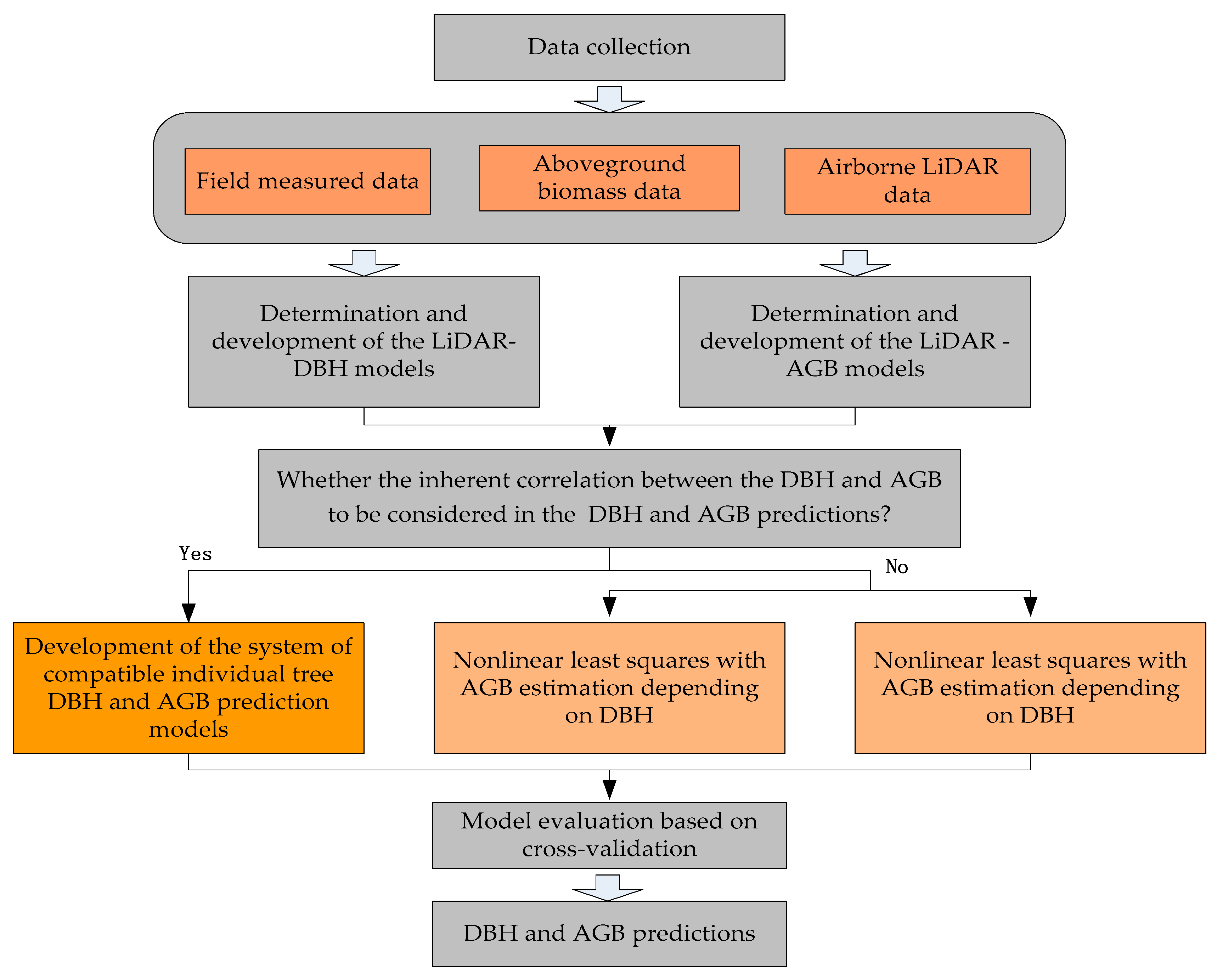
2. Materials and Methods

In Figure 1, we present a flowchart showing the development of the system of compatible individual tree DBH and AGB prediction models using error-in-variable regressions and airborne LiDAR data. The framework included the following steps: (1) collecting field measurements and LiDAR data; (2) deriving the values of LiDAR-derived tree height and crown projection area based on LiDAR point cloud data; (3) determining and developing the LiDAR–DBH and –AGB models; (4) developing the system of compatible individual tree DBH and AGB prediction models using error-in-variable regressions and two algorithms, i.e., two-stage error-in-variable model (TSEM) and nonlinear seemingly unrelated regression (NSUR); (5) evaluating and comparing the prediction accuracies of the system of compatible individual tree DBH and AGB models with those of the two parameter estimation methods (TSEM and NSUR) and of other two model structures (NLS with AGB estimation depending on DBH (NLS&DD) and NLS with AGB estimation not depending on DBH (NLS&NDD)) using a leave-one-out cross-validation approach.

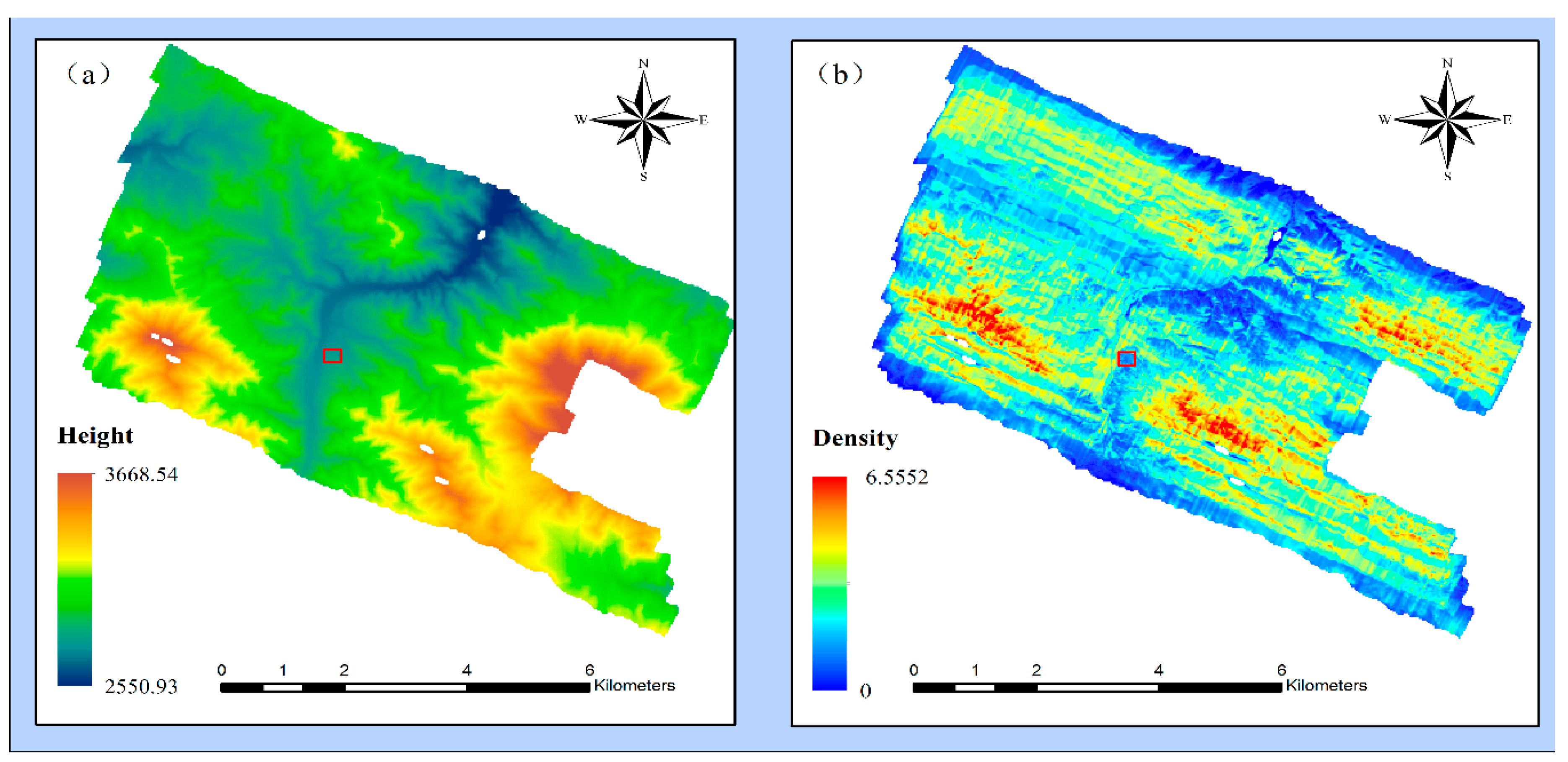
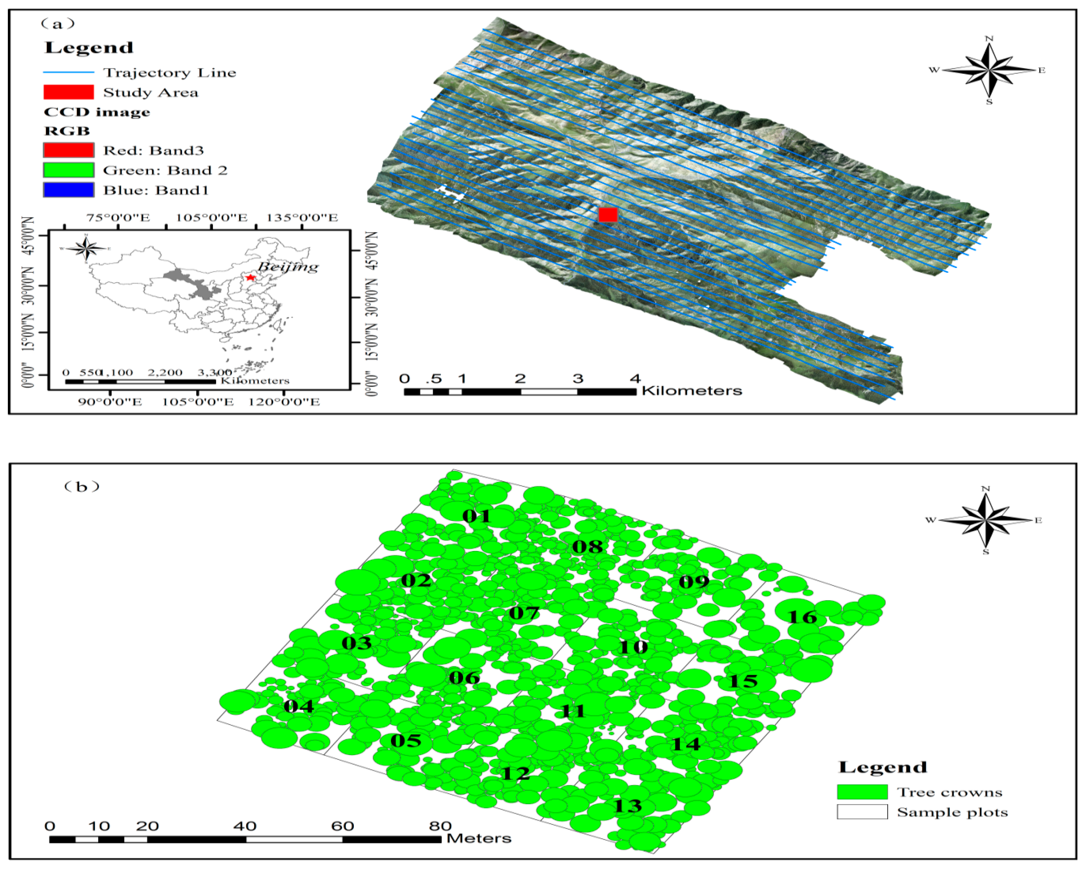
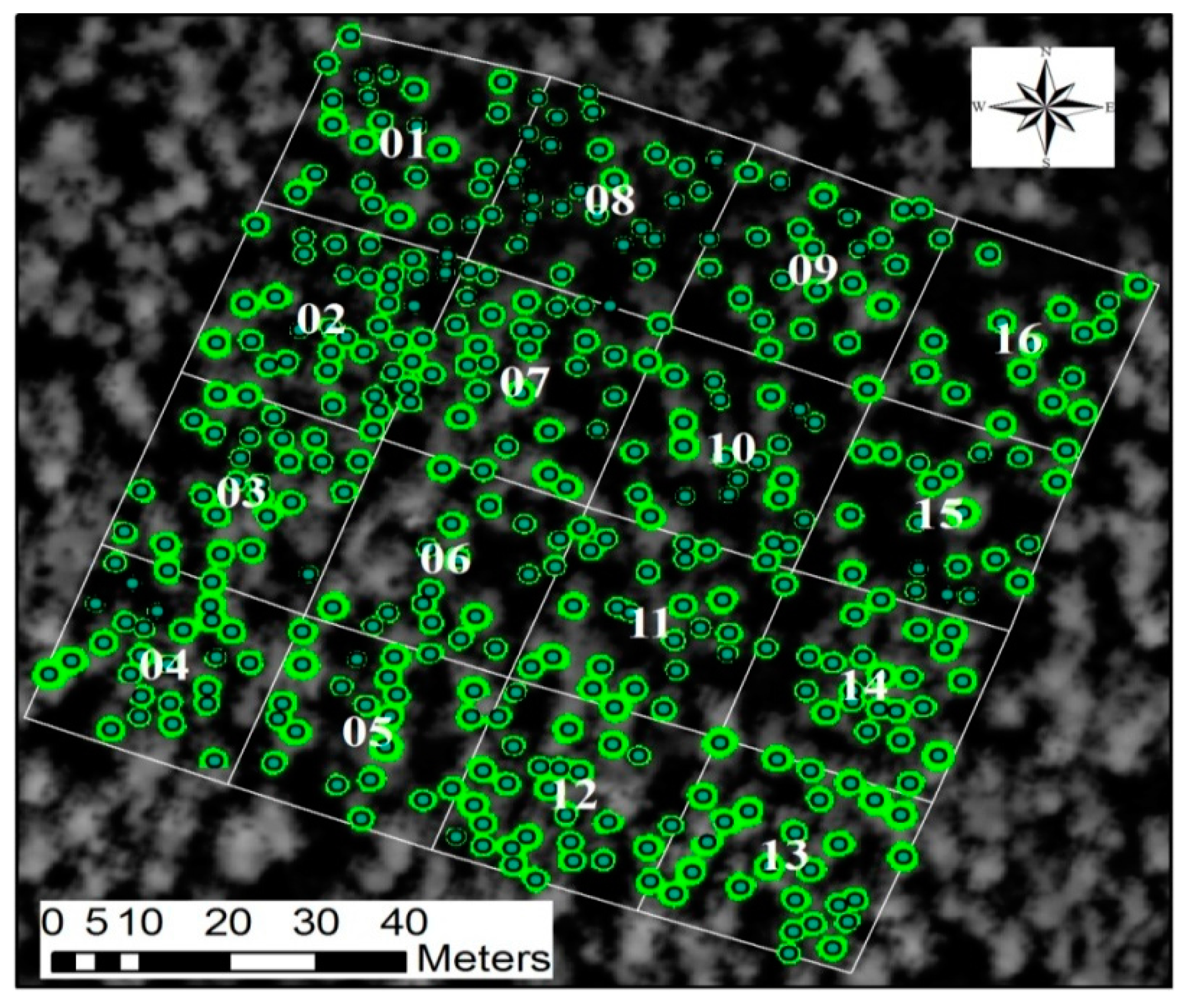
2.1. Study Area and Data

The study area is located at the Xishui forest farm of Su’nan Yuguzu Autonomous County, China, in Gansu Qilian Mountain National Nature Reserve (38°29′–38°35′N, 100°12′–100°20′E) (Figure 2a) and lies within the temperate alpine cold semi-arid and semi-humid zone. The elevation ranges from 2550 to 3680 m above sea level with an average value of 2993 m. This area is characterized by mountainous forests and steppe, and the forests were established for the purpose of water resource conservation in the Dayekou Basin of the Qilian Mountains [34,35]. Sunny and shady slopes are respectively dominated by grass and natural mature secondary pure forests. The forests are dominated by Picea crassifolia Kom. with a moss floor.

A single permanent sample plot (PSP) of 100 m × 100 m was established along the hillside and divided into sixteen subplots of 25 m × 25 m (Figure 2b). Within each of the subplots, all standing living trees with DBH larger than 5 cm were measured for DBH, tree height (H), crown base height and crown diameters in two perpendicular directions. The corners and centers of the PSP and all the subplots were measured using a differential global positioning system unit. The positions of individual trees were measured using a total station, and the spatial distribution of the tree locations is shown in Figure 2b.

Airborne LiDAR data were acquired on 23 June 2008, using a LiteMapper 5600 system. The laser scanner was Riegl LMS-Q560 (RIEGL Laser Measurement Systems GmbH: Horn, Austria) with a wavelength of 1550 nm, pulse length of 3.5 ns, and laser beam divergence of 0.5 mrad. The pulse repetition frequency was 50 kHz, the maximum scanning angle was 30°, and the scanning frequency was 49 Hz. The mean flight height was 3699 m above sea level and the mean flight speed was 230 km h⁻¹. Figure 2a shows the spatial configuration of the flight lines. The elevation of the point returns varied from 2725 to 3193 m above sea level (Figure 3a), and the mean density was 4.34 points m⁻² (Figure 3b).

2.2. LiDAR-Derived Individual Tree Characteristics

To develop LiDAR-based DBH and AGB prediction models, LiDAR-derived individual tree characteristics, such as individual tree LiDAR-derived tree height and crown projection area, should first be obtained based on LiDAR point cloud data. In this study, the individual tree crown delineation from the airborne LiDAR point cloud data was conducted on the basis of a canopy height model which was derived as the difference between the digital surface model and the digital elevation model of the study area [36,37]. The digital surface model grid was interpolated from the raw LiDAR point cloud data by a maximum height interpolation method and by filling null cells using neighbor cells [15,38]. The digital surface model contained elevation information for all objects and ground features, including trees and other natural objects. To obtain the absolute vegetation heights from the raw LiDAR point cloud data, the influence of the terrain had to be removed. Thus, the digital elevation model was used for the normalization of the raw LiDAR point heights. In this study, the digital elevation model was derived from the ground-classified LiDAR points using a progressive morphological filter [39]. The cell size of the grid was a key parameter in constructing the canopy height model [39]. Selecting an appropriate cell size should reduce the number of data gaps and ensure that sufficient detail is preserved. According to Chen et al. [40], a grid cell size of 0.5 m was applied. In addition, a Gaussian smoothing filter was also used to reduce data noise [41]. The smoothed canopy height model eliminated most of the noise and empty sinks, thus allowing a more accurate interpretation of tree crowns [42], and was finally used to obtain the LiDAR-derived tree heights and crown projection areas of individual trees.

There are two widely used methods based on a canopy height model for individual tree crown delineation. In the first method, local maxima are used as seed points for potential crown tops, and the boundary of a tree crown is then delineated using a region growing method [15,36,38,43]. This method relies on the rules of crown constraint [38,43]. In the second method, the canopy height model is first segmented into homogeneous polygons by an image segmentation algorithm [44]. The boundary of each polygon is considered as the boundary of a tree crown, and the maximum in each polygon is referred to as the crown top [44]. Relative to the second method, the first method often leads to more accurate results and was thus used in this study [38,45]. The local maxima algorithm was used to search for the tree crown tops, and the region growing algorithm was constrained by the shape features of the tree crowns. If the value of a pixel in the canopy height model was denoted with $V_{i,j}$ ($i$ and $j$ meant the $i$th row and the $j$th column of the canopy height model grid, respectively), the radius of a search window was $r$ and the increased distance from top to edge of a tree crown was denoted with $k$, the initial tree tops $f(i,j,k)$ were determined using a set of the pixels with the largest values within the search window on the basis of the following function:

$$f(i,j,k)=\{\begin{array}{l}1\mathrm{if}{V}_{i,j}>V_{i+k,j+k}\\ 0\mathrm{if}{V}_{i,j}\le V_{i+k,j+k}\end{array}-r\le k\le r$$

(1)

The crown edge pixels were constrained according to the relationship of the span angles of the crown pixels. If the top height of the current tree crown was denoted with $H_0$, the current pixel height of the crown was denoted with $H_1$, the horizontal distance between the top pixel and the current pixel was denoted with $S$, the tangent of the span angle of the top pixel ($\tan (\alpha )$) was then defined as the ratio of $S$ to $H_0$, and the tangent of the span angle of the current pixel ($\tan (\beta )$) was defined as the ratio of $S$ to $H_1$. The constraint rule was that the sum of $\tan (\alpha )$ and $\tan (\beta )$ was less than a given threshold $T$ (Equation (2)).

$$\tan (\alpha )+\tan (\beta )=\frac{S}{H_0}+\frac{S}{H_1}<T$$

(2)

It should be noted that the size of the search window was variable in this study and was determined according to the relationship between tree height and crown. In addition, two constraints for the size of the search window were applied for the determination of the crown tops: the size of the search window should be greater than or equal to the minimum crown width but less than or equal to the total tree height [45]. The crown projection area and LiDAR-derived tree height were calculated when the boundary of a tree crown was determined. The crown angle recognition algorithm and the whole crown delineation approach used in this study have been described in detail by several authors [38,45]. The rSTree algorithm was used for matching LiDAR and field trees automatically [46]. This algorithm uses the acceptable maximum Euclidian distance and minimum height difference computed between LiDAR and field-based data, in terms of tree location and height, respectively, as the imputed parameters [46]. The details of the rSTree algorithm can be found in Silva et al. [46] and are therefore not discussed in this paper.

On the basis of the aforementioned crown delineation and tree location matching approaches, a total of 402 individual P. crassifolia tree crowns in the 16 subplots nested in the PSP were delineated. The recognized individual tree crowns (outer light green area) are shown in Figure 4. Generally, for forest biomass modelling based on remote sensing data, it is impossible to obtain field measurements of forest biomass for a study area except by using a destructive method which is extremely time-consuming and costly. One appropriate and widely used method to obtain the values of forest biomass is to measure significantly correlated tree variables, such as DBH and H, and then estimate tree biomass using the developed and accurate empirical allometric models by tree species [47]. This method is very effective and accurate enough for collecting biomass data, especially in the remote sensing relevant literature [47]. Therefore, the values of the biomass components (stem, branch, foliage, and fruit) of the 402 P. crassifolia trees were estimated using the commonly used empirical allometric models developed by Wang et al. [47] and are listed in

Table 1. Empirical models with known parameters of tree biomass components (stem, branch, foliage, and fruit) for Picea crassifolia Kom. in northwestern China, sourced from Wang et al. [47] ($W_{stem}$, stem biomass; $W_{Branch}$, branch biomass; $W_{Foliage}$, branch biomass; $W_{Fruit}$, fruit biomass; DBH, diameter at breast height; and H, total height).

Component	Models
Stem	$W_{Stem}=0.0478{(DB{H}^2\times H)}^{0.8665}$
Branch	$W_{Branch}=0.0061{(DB{H}^2\times H)}^{0.8905}$
Foliage	$W_{Foliage}=0.2650{(DB{H}^2\times H)}^{0.4701}$
Fruit	$W_{Fruit}=0.0342{(DB{H}^2\times H)}^{0.5779}$

on the basis of the field-measured individual DBH and total tree height H. The AGB value of each tree was obtained by summing the component biomass values. All the estimated biomass values were applied as reference values to develop the system of compatible individual tree DBH and AGB models based on the LiDAR point clouds and also to assess the accuracies of the methods used in this study. The variables used in this study were: field-measured DBH, estimated AGB, LiDAR-derived tree height, and delineated crown projection area. The summary statistics of the four variables for the 402 trees are listed in

Table 2. Summary statistics of tree variable measurements (SD, standard deviation; DBH, field-measured diameter at breast height; AGB, aboveground biomass; LH, LiDAR-derived tree height; and CPA, crown projection area).

Variable	Mean	SD	Min	Max
DBH (cm)	23.51	7.63	5.00	43.8
AGB (kg)	181.36	134.17	1.45	632.84
LH (m)	6.95	1.90	1.96	11.30
CPA (m2)	7.43	2.06	2.94	13.50

.

2.3. Determination of the Base Model

Based on the airborne LiDAR data, DBH and AGB of individual trees are potentially correlated with two groups of variables (LiDAR-derived tree-level variables: crown projection area, LiDAR-derived tree height, and crown diameter; and LiDAR-derived stand-level variables, such as stand canopy density), which could be obtained by existing methods and algorithms with a high estimation accuracy [48,49,50]. In this study, we selected the variables using a graphical analysis of the data and an examination of correlation statistics. Moreover, the different combinations of the variables and their logarithmic transformations were also examined in both the LiDAR–DBH and the LiDAR–AGB models. To avoid over-parameterization and collinearity in the models, we selected only those variables showing significant contributions to the variations of DBH and AGB. It was found that the crown projection area and the LiDAR-derived tree height were strongly correlated with DBH and AGB, which significantly (p < 0.05) contributed to improving the predictions of DBH and AGB.

2.3.1. LiDAR–DBH Model

In this study, a base model used to develop DBH estimation models was determined from four commonly used candidate model forms, with predictor variables including the crown projection area and the LiDAR-derived tree height (

Table 3. Four candidate base models for diameter at breast height (DBH) estimation and their evaluation statistics (${\overline{\epsilon }}_{\mathrm{DBH}}$, mean prediction error; ${\sigma }^2$, variance of the biases; RMSE, root mean square error; $R^2$, coefficient of determination; ${\beta }_1-{\beta }_4$, model parameters; ${\epsilon }_{\mathrm{DBH}}$, error term; LH, LiDAR-derived tree height; CPA, crown projection area).

Model No.	Model	Model Form	${\overline{\mathit{\epsilon }}}_{\mathbf{DBH}}$	${\mathit{\sigma }}^2$	RMSE	${\mathit{R}}^2$
I.1	$\mathrm{DBH}={\beta }_1+{\beta }_{2}LH+{\beta }_{3}CPA+{\epsilon }_{\mathrm{DBH}}$	Linear	0.0000	5.8187	5.8187	0.5140
I.2	$\mathrm{DBH}={\beta }_1[1-\exp (-{\beta }_{2}LH-{\beta }_{3}CPA)]+{\epsilon }_{\mathrm{DBH}}$	Richards	0.0777	5.8294	5.8300	0.5122
I.3	$\mathrm{DBH}={\beta }_1/[1+{\beta }_2\exp (-{\beta }_{3}LH-{\beta }_{4}CPA)]+{\epsilon }_{\mathrm{DBH}}$	Logistic	0.0028	5.7569	5.7569	0.5243
I.4	$\mathrm{DBH}={\beta }_1\exp (-{\beta }_{2}LH-{\beta }_{3}CPA)+{\epsilon }_{\mathrm{DBH}}$	Exponential	−0.0025	5.7584	5.7584	0.5241

), on the basis of the performance of model fitting using the full data set. All tested models had three parameters, except for model I.3 (four parameters). Nonlinear regressions were carried out using the NLS technique nls (nonlinear least squares) function in the version 3.2.2 of the R software [51]. The base model with the best performance was selected using the following four statistical criteria [52]:

$$R^2=1-{\displaystyle \sum {(DB{H}_i-D\widehat{B}{H}_i)}^2}/{{\displaystyle \sum (DB{H}_i-\overline{DBH})}}^2$$

(3)

$$\overline{\epsilon }={\displaystyle \sum {\epsilon }_i/N}={\displaystyle \sum (DB{H}_i-D\widehat{B}{H}_i)}/N$$

(4)

$${\sigma }^2={\displaystyle \sum {({\epsilon }_i-\overline{\epsilon })}^2/(N-1)}$$

(5)

$$\mathrm{RMSE}=\sqrt{{\overline{\epsilon }}^2+{\sigma }^2}$$

(6)

where $DB{H}_i$ and $D\widehat{B}{H}_i$ are the observed and predicted DBH for the ith observation ($i=1,\dots ,N$), N is the total number of observations, $\overline{DBH}$ is the mean of DBH observations, $R^2$ is the coefficient of determination, $\overline{\epsilon }$ is the mean bias, ${\sigma }_{}^2$ is the bias variance, and RMSE is the root mean square error that combines the mean bias and the bias variance, providing a robust measure of the overall model accuracy. Therefore, RMSE was used as the primary criterion for model evaluation.

The fitting statistics of models I.1–I.4 are presented in Table 3. Although the evaluation statistics were almost identical for the four models, and the values of RMSE did not significantly differ from each other at the significance level of 0.05, both models I.3 and I.4 showed a slightly superior fitting compared with models I.1 and I.2. Moreover, model I.4 was simpler than model I.3 as it contained only three parameters and was thus selected as the basic nonlinear model to develop compatible individual tree models for DBH based on the airborne LiDAR data.

2.3.2. LiDAR–AGB Model

The experiment of this study showed that DBH and LiDAR-derived tree height and crown projection area greatly contributed to the variability of AGB. Moreover, allometric models are most commonly used to estimate tree biomass by relating tree biomass to the easily measured tree variables [7,8]. Therefore, the one-predictor, two-predictor, and three-predictor allometric models of AGB were developed using DBH alone (model II.1 in

Table 4. Five candidate base models of aboveground biomass (AGB) estimation and their evaluation statistics (${\overline{\epsilon }}_{\mathrm{AGB}}$, mean prediction error; ${\sigma }^2$, variance of the biases; RMSE, root mean square error; $R^2$, coefficient of determination; LL, log-likelihood; LRT, likelihood ratio test; ${\alpha }_1-{\alpha }_4$, model parameters; ${\epsilon }_{AGB}$, error term; AGB, aboveground biomass; DBH, diameter at breast height; LH, LiDAR-derived tree height; CPA, crown projection area).

Model No.	Model	${\overline{\mathit{\epsilon }}}_{\mathbf{AGB}}$	${\mathit{\sigma }}^2$	RMSE	${\mathit{R}}^2$	−2LL	LRT	p Value
II.1	$\mathrm{AGB}={\alpha }_{1}DB{H}^{{\alpha }_2}+{\epsilon }_{\mathrm{AGB}}$	−4.8730	31.7568	32.1285	0.9427	−1965	-	-
II.2	$\mathrm{AGB}={\alpha }_{1}DB{H}^{{\alpha }_2}L{H}^{{\alpha }_3}+{\epsilon }_{\mathrm{AGB}}$	0.4477	18.2123	18.2178	0.9816	−1737	228	<0.0001
II.3	$\mathrm{AGB}={\alpha }_{1}DB{H}^{{\alpha }_2}CP{A}^{{\alpha }_3}+{\epsilon }_{\mathrm{AGB}}$	−0.5761	20.6800	20.6880	0.9762	−1788	177	<0.0001
II.4	$\mathrm{AGB}={\alpha }_{1}L{H}^{{\alpha }_2}CP{A}^{{\alpha }_3}+{\epsilon }_{\mathrm{AGB}}$	1.9894	91.6294	91.6501	0.5334	−2386	421	<0.0001
II.5	$\mathrm{AGB}={\alpha }_{1}DB{H}^{{\alpha }_2}L{H}^{{\alpha }_3}CP{A}^{{\alpha }_4}+{\epsilon }_{\mathrm{AGB}}$	0.4645	18.2086	18.2145	0.9816	−1737	228	<0.0001

), pairwise combinations of DBH, LiDAR-derived tree height, and crown projection area (models II.2–II.5 in Table 4), and three independent variables, i.e., DBH, LiDAR-derived tree height, and crown projection area, together (model II.5 in Table 4), respectively. To account for the heteroscedasticity, a power weight function with DBH as a predictor ($\mathrm{var}(\epsilon )={\mathrm{DBH}}^{\gamma }$, γ was an estimated parameter), was applied in the AGB modeling. The five models were separately used to fit the full data set (Table 4). The resulting model with the largest log-likelihood (LL) and $R^2$ and the smallest RMSE was selected as the base model of AGB. To avoid the problems caused by over-parameterization, we performed a likelihood ratio test, which is a test of the sufficiency of a simpler model versus a more complex model [53].

On the basis of the fitting statistics in Table 4, both models II.2 and II.5 showed a significantly superior fitting (with almost identical fitting accuracy), compared with the other three models (p < 0.0001). Relative to model II.5, model II.2 was simpler, with only two predictors. Therefore, model II.2 was selected as the basic model of AGB for further analyses.

2.4. A System of Compatible Individual Tree DBH and AGB Error-In-Variable Models

The above LiDAR–DBH and LiDAR–AGB base models were called base submodels [3]. According to the error-in-variable modeling approach proposed by Fu et al. [3] and Tang et al. [29,30], integrating these two submodels led to a system of error-in-variable models for estimating individual tree DBH and AGB as follows:

$$\{\begin{array}{l}db{h}_i={\beta }_1\exp \left[-{\beta }_{2}L{H}_i-{\beta }_{3}CP{A}_i\right]\\ ag{b}_i={\alpha }_{1}db{h}_i^{{\alpha }_2}L{H}_i^{{\alpha }_3}\\ DB{H}_i=db{h}_i+{\epsilon }_{DBHi}\\ AG{B}_i=ag{b}_i+{\epsilon }_{AGBi}\end{array}$$

(7)

where $DB{H}_i$ and $AG{B}_i$($i=1,\dots ,N$) were the field-measured values of the diameter at breast height (cm) and the estimated values of aboveground biomass (kg) of the $i\mathrm{th}$ tree, respectively, and the values contain random errors; $db{h}_i$ and $ag{b}_i$ were the true values (errors free) of $DB{H}_i$ and $AG{B}_i$, respectively; $L{H}_i$ and $CP{A}_i$ were the LiDAR-derived tree height (m) and crown projection area (m²) of the $i\mathrm{th}$ tree, respectively; $N$ was the total number of trees; and ${\beta }_1-{\beta }_3$ and ${\alpha }_1-{\alpha }_3$ were the model parameters; ${\mathsf{\epsilon }}_i={({\epsilon }_{DBHi},{\epsilon }_{AGBi})}^T$ were normally distributed two-dimensional vectors with zero means and respective variance–covariance matrix $\Sigma$. The variance–covariance matrix $\Sigma$ with $2\times 2$ dimensions was used to account for the inherent correlation between DBH and AGB [30,49]. Both DBH and AGB were considered as error-in variables in this study. The crown projection area and LiDAR-derived tree height in the model system (7) were assumed as error-out variables. The observed values of these variables were assumed as true values. The detailed steps for estimating individual tree DBH and AGB using the model system (7) were as follows: the parameters in the model system were first estimated, and then the DBH estimates ($D\widehat{B}H$) were calculated by the LiDAR–DBH base submodel with the estimated parameters and the observed values of LiDAR-derived tree height and crown projection area, and the AGB estimate was finally obtained by the LiDAR–AGB base submodel with the estimates $D\widehat{B}H$ and the observed values of LiDAR-derived tree height.

2.4.1. Structure for the Variance–Covariance Matrix $\Sigma$

The assumption of the model system (7) was that the error terms ${\epsilon }_{ti}$($t=$ DBH and AGB; and $i=1,\dots ,N$) were independent across different sample trees but had cross-equation contemporaneous correlations. Thus, we assumed that

$$E({\epsilon }_{t_1{i}_1},{\epsilon }_{t_2{i}_2}|X)=\{\begin{array}{l}0,\mathrm{whenever}{i}_1\ne i_2,i_1,i_2=1,\dots ,N;t_1,t_2=\mathrm{DBH},\mathrm{AGB}\\ {\sigma }_{t_1{t}_2},\mathrm{whenever}{i}_1=i_2\end{array}$$

(8)

where

$$\underset{2N\times k}{X}=\left(\begin{array}{cc}\underset{N\times 3}{X_{\mathrm{DBH}}}& \\ & \underset{N\times 3}{X_{\mathrm{AGB}}}\end{array}\right)$$

(9)

was the $2N\times k$ block diagonal design matrix of $\mathsf{\theta }={({\mathsf{\beta }}_{\mathrm{DBH}}^T,{\mathsf{\alpha }}_{\mathrm{AGB}}^T)}^T$ (${\mathsf{\beta }}_{\mathrm{DBH}}^{}={({\beta }_1,{\beta }_2,{\beta }_3)}^T$ and ${\alpha }_{\mathrm{AGB}}={({\alpha }_1,{\alpha }_2,{\alpha }_3)}^T$), $k=6$ was the total number of parameters in the model system (7), and $X_t$ ($t=$ DBH and AGB) was the $N\times 3$ design matrix of the partial derivates with respect to the parameter vector ${\mathsf{\beta }}_t$ (or ${\mathsf{\alpha }}_t^{}$) in the $i\mathrm{th}$ submodel. Therefore, $\mathsf{\Sigma }$ was a $2\times 2$ conditional variance or heteroscedasticity matrix of each observation, as given below:

$$\mathsf{\Sigma }={[{\sigma }_{t_1{t}_2}]}_{2\times 2}=\left(\begin{array}{cc}{\sigma }_{\mathrm{DBH}\times \mathrm{DBH}}& {\sigma }_{\mathrm{DBH}\times \mathrm{AGB}}\\ {\sigma }_{\mathrm{AGB}\times \mathrm{DBH}}& {\sigma }_{\mathrm{AGB}\times \mathrm{AGB}}\end{array}\right)$$

(10)

The covariance matrix of the stacked error terms ($\epsilon ={({\epsilon }_{\mathrm{DBH}}^T,{\epsilon }_{\mathrm{AGB}}^T)}^T$ (${\epsilon }_t={({\epsilon }_{t1},\dots ,{\epsilon }_{tN})}^T$, $t=$ DBH and AGB) would be

$$\underset{2N\times 2N}{R}=E({\epsilon }^T\epsilon |X)=\underset{2\times 2}{\mathsf{\Sigma }}\otimes I_N$$

(11)

The inherent correlation between the DBH and AGB in the model system (7) was accounted for by $\mathsf{\Sigma }$.

2.4.2. Parameter Estimation Methods

In this study, the model parameter vector $\mathsf{\theta }={({\mathsf{\beta }}_{\mathrm{DBH}}^T,{\mathsf{\alpha }}_{\mathrm{AGB}}^T)}^T$ in the model system (7) was estimated by applying the TSEM algorithm and NSUR, respectively.

(I) TSEM algorithm

The model system (7) was solved using the following two steps with the TSEM algorithm [31]:

Step 1: set $\mathsf{\Sigma }=I$ and estimate the parameter vector $\mathsf{\theta }$ by minimizing the following objective function:

$$Q_1(y_i,\mathsf{\theta })={\displaystyle \sum _{i=1}^N(Y_i-y_i){\Sigma }^{-1}{(Y_i-y_i)}^T}$$

(12)

where $Y_i={(DB{H}_i,AG{B}_i)}^T$ are the observed values of the 2-dimensional error-in variables, and $y_i={(db{h}_i,ag{b}_i)}^T$ is the true value of $Y_i$, which is equal to the expectation [$y_i=E(Y_i)$] defined by the right-hand sides of the submodels in the model system (7). Then, the estimates of all elements in the variance–covariance matrix, $\widehat{\Sigma }$, were obtained by calculating ${\widehat{\mathsf{\epsilon }}}_t$($t=\mathrm{DBH}\mathrm{and}\mathrm{AGB}$), using the model system (7) with the observations $Y_i$ and two error-out variables $x_i=(L{H}_i,CP{A}_i)$:

$${\widehat{\sigma }}_{t_1{t}_2}=({\widehat{\epsilon }}_{t_1}^T{\widehat{\epsilon }}_{t_2})/\sqrt{(N-3)(N-3)}(t_1,t_2=\mathrm{DBH},\mathrm{AGB})$$

(13)

Step 2: the final estimate of $\mathsf{\beta }$ was obtained by minimizing the objective function:

$$Q_2(y_i,\mathsf{\theta })={\displaystyle \sum _{i=1}^n(Y_i-y_i){\widehat{\Sigma }}^{-1}{(Y_i-y_i)}^T}$$

(14)

and the variance of $\mathsf{\theta }$ was given by:

$$\mathrm{cov}(\widehat{\mathsf{\theta }})={\left({\underset{6\times 2N}{X}}^T\left(dg({({\underset{2\times 2}{\widehat{\mathsf{\Sigma }}}}^{-1})}^{-1})\otimes I_N\right)\underset{2N\times 6}{X}\right)}^{-1}$$

(15)

where $dg()$ denotes extracting the diagonal elements of a matrix.

This TSEM algorithm was implemented in ForStat 2.1 software [54]. The details of parameter estimation and computer implementation of TSEM can be found in [29,30].

(II) NSUR

The model system (7) was also estimated by NSUR using a feasible generalized least square method in the following two steps [30]:

Step 1: the NLS was applied to separately fit the two submodels in the model system (7) to the dataset to obtain model residuals ${\widehat{\epsilon }}_t$($t=$ DBH and AGB) which were used to estimate the elements of the matrix $\Sigma$.

Step 2: a generalized least square was used to estimate the parameter vector using an estimate of the covariance matrix $\widehat{R}=\widehat{\Sigma }\otimes I_N$, as follows:

$$\widehat{\mathsf{\theta }}={({\underset{6\times 2N}{X}}^T({\underset{2\times 2}{\widehat{\Sigma }}}^{-1}\otimes I_N)\underset{2N\times 6}{X})}^{-1}{\underset{6\times 2N}{X}}^T({\underset{2\times 2}{\widehat{\Sigma }}}^{-1}\otimes I_N)\underset{2N\times 1}{y}$$

(16)

and

$$\mathrm{cov}(\widehat{\mathsf{\theta }})={\left({\underset{6\times 2N}{X}}^T\left({({\underset{2\times 2}{\widehat{\Sigma }}}^{-1})}^{-1}\otimes I_N\right)\underset{2N\times 6}{X}\right)}^{-1}$$

(17)

For more details of NSUR, readers are referred to the studies in [55,56,57,58,59].

2.5. Other Model Structures for Comparison

2.5.1. Nonlinear Least Squares with AGB Estimation Depending on DBH

Base models I.4 in Table 3 and II.2 in Table 4 were separately utilized to fit the dataset by the NLS&DD approach to quantify the consequences of using a prediction of DBH to replace an actual value without accounting for the error in a predicted DBH for estimating AGB. The estimates of $DB{H}_i$ and $AG{B}_i$ ($i=1,\dots ,N$) were derived as follows:

$$D\widehat{B}{H}_i={\widehat{\beta }}_1\exp (-{\widehat{\beta }}_{2}L{H}_i-{\widehat{\beta }}_{3}CP{A}_i)$$

(18)

$$A\widehat{G}{B}_i={\widehat{\alpha }}_{1}D\widehat{B}{H}_i^{{\widehat{\alpha }}_2}L{H}_i^{{\widehat{\alpha }}_3}$$

(19)

where $D\widehat{B}{H}_i$ in Equation (19) were obtained from Equation (18). NLS&DD ensured the compatibility between the estimates of $DB{H}_i$ and $AG{B}_i$, but the inherent correlation between the two variables could not be addressed. In addition, the effect of errors in $D\widehat{B}{H}_i$ on $AG{B}_i$ prediction for this model structure was also ignored.

2.5.2. Nonlinear Least Squares with AGB Estimation Not Depending on DBH

The DBH in the base model II.2 in Table 4 could also be replaced directly by the base model I.4 in Table 3. Therefore, the AGB estimation using this method was independent of DBH. The modified AGB model was given by

$$AG{B}_i={\alpha }_{1}DB{H}_i^{{\alpha }_2}L{H}_i^{{\alpha }_3}+{\epsilon }_{AGBi}={\gamma }_1\exp (-{\gamma }_{2}L{H}_i-{\gamma }_{3}CP{A}_i)L{H}_i^{{\gamma }_4}+{\tilde{\epsilon }}_{AGBi}$$

(20)

where ${\gamma }_1={\alpha }_1{\beta }_1{}^{{\alpha }_2}$, ${\gamma }_2={\alpha }_2{\beta }_2$, ${\gamma }_3={\alpha }_2{\beta }_3$, and ${\gamma }_4={\alpha }_2$ were the model parameters, and the new error term was

$${\tilde{\epsilon }}_{AGBi}=f(L{H}_i,CP{A}_i){\epsilon }_{DBHi}+{\epsilon }_{AGBi},$$

(21)

in which

$$f(L{H}_i,CP{A}_i)={\alpha }_1{\alpha }_2{\beta }_1^{({\alpha }_2-1)}\exp \left[-{\beta }_2({\alpha }_2-1)L{H}_i-{\beta }_3({\alpha }_2-1)CP{A}_i\right]L{H}_i^{{\alpha }_3}.$$

(22)

The $DB{H}_i$ and $AG{B}_i$ ($i=1,\dots ,N$) were estimated by model I.4 in Table 3 and model (20), respectively, with known parameters fitted by NLS&NDD. However, NLS&NDD could not ensure the compatibility between the estimates of $DB{H}_i$ and $AG{B}_i$. The inherent correlation between the two variables also could not be addressed by this method.

2.6. Evaluation and Comparison of Model Predictions Based on a Leave-One-Out Cross-Validation Approach

The validity of the DBH and AGB estimation models could be evaluated using an independent dataset [60]. However, such a validation procedure was not feasible in this study because of the limited data collected. Instead, the predictive ability of the DBH and AGB estimation models was evaluated using a leave-one-out cross-validation approach [61,62]. We deleted a tree from the full dataset (Table 2), fitted the DBH and AGB estimation models with the data on the basis of the remaining observations, and used the obtained parameters to predict DBH and AGB for the deleted tree. Then, we put this tree back, removed a different tree and conducted the same modeling and estimation procedure. This process was conducted for all 402 trees in the data set. The observed and predicted DBH and AGB values of the trees were finally utilized to calculate $\overline{e}$, $\delta$, RMSE, and $R^2$ (Equations (3)–(6)). The predictive abilities of the model system (7) with TSEM, NSUR, NLS&DD, and NLS&NDD parameter estimation approaches were compared on the basis of the results of the leave-one-out cross-validation. The model with the smallest $\overline{e}$, $\delta$, and RMSE, and the largest $R^2$ was selected to estimate both DBH and AGB. All calculations were conducted using R version 3.2.2 software (The R Foundation for Statistical Computing: Vienna, Austria).

3. Results

3.1. Estimation of the Parameters

Table 5. Parameter estimates of model I.4 in Table 3, model II.2 in Table 4, and model (20) fitted by nonlinear least squares, and of model system (7) fitted by nonlinear seemingly unrelated regression (NSUR) and two-stage error-in-variable model (TSEM) using the full dataset (DBH, diameter at breast height; AGB, aboveground biomass).

Parameters	Model I.4	Model II.2	Model (20)	Model System (7)
				NSUR	TSEM
DBH-related parameters
${\beta }_1$(${\gamma }_1$)	8.6595	_	10.9351	8.5799	8.2213
${\beta }_2$(${\gamma }_2$)	−0.0851	_	-0.1117	−0.0863	−0.0894
${\beta }_3$(${\gamma }_3$)	−0.05	_	−0.0879	−0.0501	−0.0522
AGB-related parameters
${\alpha }_1$(${\gamma }_4$)	_	0.2267	0.6457	0.2307	0.2386
${\alpha }_2$	_	1.7701	_	1.7594	1.7435
${\alpha }_3$	_	0.5008	_	0.5095	0.5188
Variance components
${\sigma }_{DD}$	_	_	_	33.3283	33.4050
${\sigma }_{DW}$	_	_	_	13.1971	20.2866
${\sigma }_{WW}$	_	_	_	334.7768	340.1165
${\sigma }^2$	5.773	18.26	91.64	_	_

lists the parameter estimates of models I.4 in Table 3, II.2 in Table 4, and model (20) by NLS, and of the model system (7) by NSUR and TSEM using the full data set. All the parameter estimates of the models were highly significant (p < 0.05), and their magnitudes and signs were also biologically plausible. It should be noted that all elements ${\sigma }_{t_1{t}_2}$($t_1,t_2=$ DBH and AGB) in $\Sigma$ for the model system (7) for both NSUR and TSEM were significantly different from 0 (p < 0.05), indicating that the correlation between DBH and AGB was statistically significant.

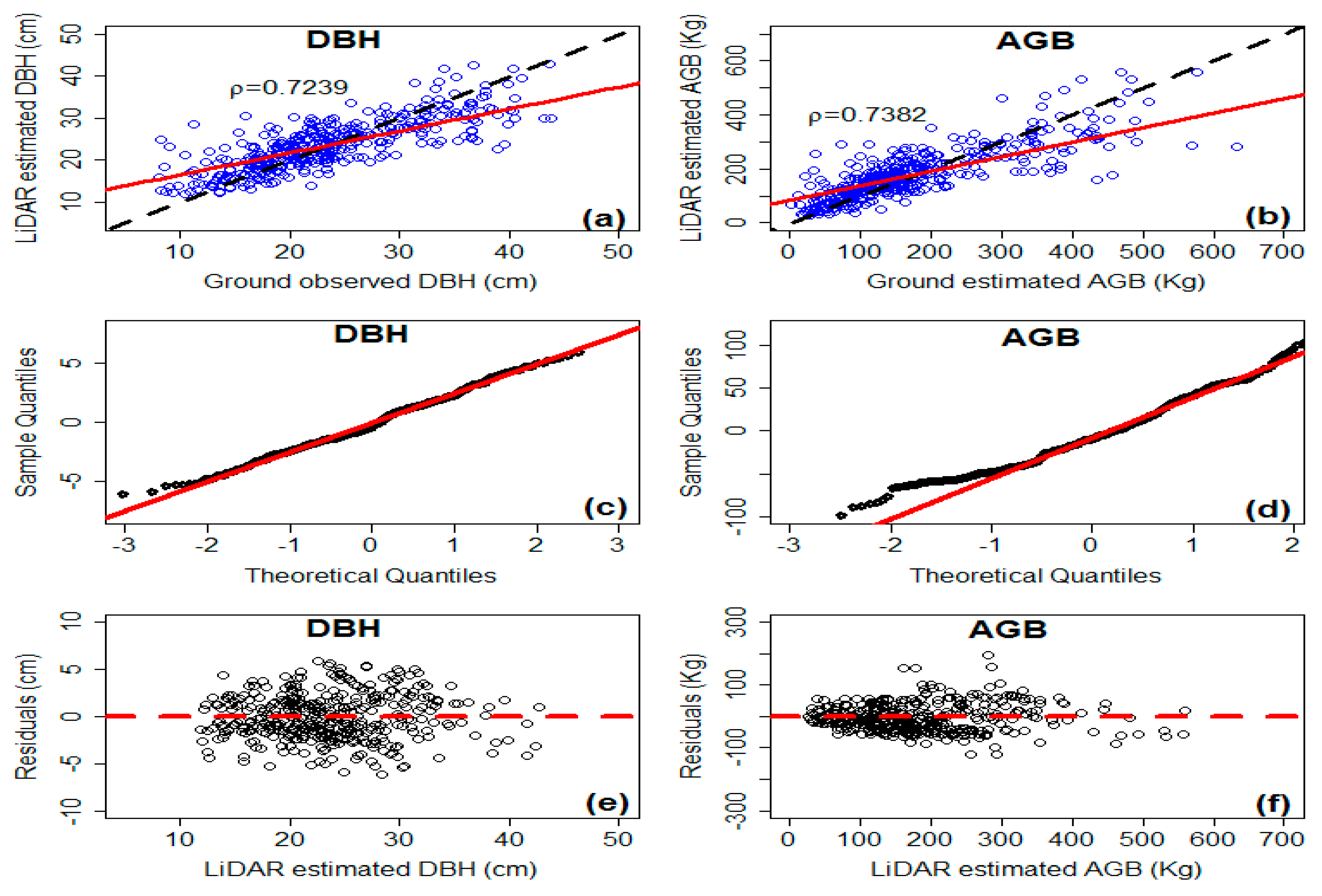
3.2. Model Evaluation

The comparisons of DBH and AGB predictions were made among NLS&DD (Model I.4 in Table 3 and Model II.2 in Table 4), NLS&NDD (Model I.4 in Table 3 and Model (20)), and model system (7) with both NSUR and TSEM based on the leave-one-out cross-validation. The error statistics for the predictions of these models are presented in

Table 6. Comparison of the performance of the four methods: nonlinear least square (NLS) with AGB estimation depending on DBH (NLS&DD), NLS with AGB estimation not depending on DBH (NLS&NDD), model system (7) with nonlinear seemingly unrelated regression (MS-NSUR), and model system (7) with two-stage error-in-variable model (MS-TSEM), for individual tree diameter at breast height (DBH) and aboveground biomass (AGB) by the mean prediction error ($\overline{e}$), variance of the biases (${\sigma }^2$), root mean square error ($RMSE$), and coefficient of determination ($R^2$) using the leave-one-out cross-validation.

Model	$\overline{\mathit{e}}$	$\mathit{\delta }$	$\mathbf{RMSE}$	${\mathit{R}}^2$
NLS&DD
$\mathrm{DBH}$	−0.0028	5.8341	5.8341	0.5193
$\mathrm{AGB}$	6.5972	91.3987	91.6365	0.5335
NLS&NDD
$\mathrm{DBH}$	−0.0028	5.8341	5.8341	0.5193
$\mathrm{AGB}$	0.0581	91.2973	91.2973	0.5370
MS-NSUR
$\mathrm{DBH}$	0.0097	5.7587	5.7587	0.5251
$\mathrm{AGB}$	6.5559	91.0211	91.2569	0.5449
MS-TSEM
$\mathrm{DBH}$	0.0648	5.7649	5.7653	0.5239
$\mathrm{AGB}$	6.1813	91.0873	91.2968	0.5430

. The simple Student’s t-test showed that the mean biases for all models were not significantly different from zero (p > 0.05) for DBH predictions, but they were significantly different from zero (p < 0.05) for AGB predictions. For DBH, both NLS&DD and NLS&NDD had a small overprediction, while the model system (7) with both NSUR and TSEM showed a small underprediction. All models showed a large underprediction for AGB.

The prediction accuracies of both DBH and AGB from the model system (7) with NSUR were slightly higher than those from the model system (7) with TSEM, NLS&DD, and NLS&NDD. For example, for DBH, the RMSE of the model system (7) with NSUR was 5.7587, which was 0.15%, 1.29%, and 1.29% smaller than those from model system (7) with TSEM, NLS&DD, and NLS&NDD, respectively. For AGB, the $R^2$ of the model system (7) with NSUR was 0.5449, which was 0.35%, 1.47%, and 2.14% larger than those from model system (7) with TSEM, NLS&DD, and NLS&NDD, respectively. In particular, for both DBH and AGB, NSUR showed a slightly superior performance to TSEM. However, the discrepancy of the evaluation indices was very small.

Figure 5 shows the correlations between the observed and predicted values, distribution of residuals, and QQ plots of the model system (7) by NSUR for both DBH and AGB, on the basis of the leave-one-out cross-validation results. The correlation coefficients between the observed and predicted values of DBH and AGB were very high. The heteroscedasticity trend almost disappeared for the model system (7). This indicated that the power weight function applied to DBH effectively accounted for the heteroscedasticity. In addition, the QQ plots of the model system (7) for both DBH and AGB showed clear linear relationships for the residuals.

4. Discussion

Forests are considered as the most productive terrestrial ecosystems on Earth, containing more than 45% of the global terrestrial carbon stock [63]. Quantifying the amount of forest biomass is necessary for land managers to make informed decisions about forest management and planning [22]. In the current study, a system of compatible individual tree DBH and AGB models was developed using an error-in-variable modeling approach based on airborne LiDAR data. The measurement errors in both the dependent (AGB) and independent (DBH) variables and the correlation between DBH and AGB were taken into account in the developed model system. To make comparisons, other two widely used model structures (NLS&DD and NLS&NDD) were employed to estimate the DBH and AGB. For both NLS&DD and NLS&NDD, it was assumed that there were no measurement errors in the observed values of the independent variables, while the observed values of the dependent variable contained errors. In addition, the correlation between DBH and AGB was not considered for either of the two model structures. Thus, if the independent variables had measurement errors that were not negligible or the correlation between DBH and AGB was also highly significant, the estimates of DBH and AGB from both NLS&DD and NLS&NDD might be biased. However, the error-in-variable modeling approach can theoretically lead to unbiased estimations and is more generalized and flexible than NLS&DD and NLS&NDD [30]. These characteristics were supported by the findings of this study (Table 6).

The results of this study showed that both the crown projection area and the LiDAR-derived tree height could be used to infer individual tree DBH and AGB. This offers the potential to deploy remote sensing tools for large scale assessments of aboveground biomass stocks across entire landscapes. From a remote sensing perspective, crown projection area and LiDAR-derived tree height are much more easily measured than canopy diameter for the simple reason that the extracted crown diameter parameter is influenced by the direction of the measurement vector [19]. Numerous studies have found a strong relationship between crown diameter and DBH [64,65]. Given an established sampling regime, determining a tree crown diameter (or canopy extent) aimed at minimizing the effect of crown asymmetry [66]. Crown diameters could potentially be derived from the remotely sensed crown projection area measurements by applying appropriate shape parameters, as discussed in the studies of Fleck et al. [66], Nelson [67], and Grote [68]. The crown diameter was also examined in the current study, and it was found that its contribution to improving the prediction accuracies of the LiDAR–DBH and LiDAR–AGB models was not significant. This was mainly because (i) the crown projection area involved in the proposed LiDAR–DBH model could reflect the crown effects, and (ii) introducing the crown diameter would complicate the model, with a very little gain in predictability. Thus, the crown diameter was not selected as a predictor in the LiDAR–DBH and LiDAR–AGB models.

In this study, the results from the error-in-variable modeling demonstrated its advantages over NLS in predicting AGB when DBH was subject to measurement errors for Picea crassifolia Kom. in northwestern China (Table 6). In practice, the predictor DBH in the LiDAR–AGB models was estimated from the LiDAR–DBH model, and therefore the random errors in the estimates of DBH were unavoidable. In addition, it is also difficult to avoid the measurement errors related to tree detection including the LiDAR system, the point density, the spatial pattern, the delineation algorithm, and the geometric characteristics of the crown shape in remotely sensed imagery at an individual tree level. More importantly, the regression models developed for a given dataset cannot be applied to predict the response variable for a dataset that is significantly different from the model development dataset [30]. Lindley [69] showed that if the prediction data were from the same population as the parameter estimation data, the predictions from the NLS models were generally unbiased even if the independent variable was subject to measurement errors. However, the prediction could be biased if the parameter estimation data were taken from a different population [30].

The model system (7) fitted by both TSEM and NSUR performed better in terms of the predictions of the DBH and AGB, relative to NLS&DD and NLS&NDD (Table 6). This indicated that the model system (7) was a more effective compatible model for DBH and AGB compared to both NLS&DD and NLS&NDD. When DBH and AGB were estimated from the separately fitted LiDAR–DBH and LiDAR–AGB models using NLS&DD and NLS&NDD, the prediction accuracies of DBH from the two model structures were similar to those obtained from the traditional base model II.2 in Table 4. This was because the LiDAR–DBH models for both NLS&DD and NLS&NDD were identical to the base model II.2. However, the prediction accuracy of NLS&NDD was much higher than that of NLS&DD for AGB prediction (Table 6). For example, the value of $\overline{e}$ from the NLS&NDD was 0.0581 and 99.12% smaller than that from NLS&DD ($\overline{e}=6.5972$), and the value of $R^2$ from the NLS&NDD was 0.5370 and 0.65% larger than that from NLS&DD ($R^2=0.5335$). This was probably because the DBH in the model (20) was replaced by the corresponding LiDAR–DBH base model II.2, and thus the measurement error from the estimated DBH used to estimate AGB was effectively avoided. We also attempted to develop a compatible model system for estimating individual tree DBH and AGB using base model II.2 and model (20) as two submodels with both TSEM and NSUR, but NSUR failed to converge. More importantly, the correlation between DBH and AGB in this model could not be accounted for.

Based on the leave-one-out cross-validation results (Table 6), we found that the values of the same statistics were very similar to each other for NSUR and TSEM. However, the prediction accuracy of the model system (7) fitted by NSUR was slightly higher than that fitted by TSEM. In addition, the other main advantage of the NSUR method was that this could be readily implemented by both the R nlsystemfit (nonlinear equation system estimation) function [70] and the SAS/ETS MODEL procedure [71]. However, ForStat 2.1 software [54] is not readily available for non-Chinese modelers. It should be noted that TSEM is recommended when convergence is a big issue in model applications.

Finally, this study aimed to develop a novel methodology, that is, a system of compatible individual tree DBH and AGB error-in-variable models, in which airborne LiDAR images and reference data of tree biomass were combined to derive the LiDAR–AGB and –DBH models, and the measurement errors of both AGB and DBH were simultaneously taken into account. This made it possible to expand the error-in-variable modeling for the estimation of DBH and AGB from individual trees to stands by introducing the LiDAR data. The second objective of this study was to demonstrate the potential improvements of AGB and DBH estimates as a result of the use of the error-in-variable modeling with the NSUR and TSEM approaches by comparison with the traditional modeling methods (NLS&DD and NLS&NDD). However, the results showed that the obtained improvements statistically did not significantly differ from zero at the significant level of 0.05. The reason might be mainly that the estimates of tree DBH and AGB were associated with various source uncertainties [72,73,74]. The uncertainties might come from the measurement errors of the tree variables, the errors of the used LiDAR data, the errors in delineating the tree crowns and estimating the tree LH and DBH using the LiDAR data, the estimation errors of the used model parameters, etc. In this study, the measurement errors of both DBH and AGB were considered using the error-in-variable modeling method. Moreover, in order to decrease the estimation errors of the parameters of the empirical allometric models in Table 1, the parameter estimates of the models were obtained by a nonlinear least square based on the field measurements of DBH and H, instead of their estimates, and used to estimate the biomass values of the trees. However, other source errors were ignored in this study. This implies that, in order to validate the potential improvements of AGB and DBH estimates derived from the use of the error-in-variable modeling, a systematical analysis of uncertainty propagation is needed by identifying all the error sources, modeling their propagation from inputs to outputs, and quantifying their impacts on the estimation accuracy of AGB [72]. However, the uncertainty analysis is very complicated [72], was not conducted in this study because of a limited space, and should be carried out in a future study. Thus, readers should take caution in using the conclusions of this study.

5. Conclusions

In this study, a system of compatible individual tree DBH and AGB error-in-variable models (model system (7)) was developed using an error-in-variable modeling approach based on both the airborne LiDAR and the field-measured datasets of individual P. crassifolia trees collected in northwestern China. Two alternative parameter estimation algorithms, TSEM and NSUR, were proposed for estimating the model parameters in the developed model system (7). It was found that the parameter estimates from both TSEM and NSUR were very similar. For comparison, other two model structures, NLS&DD and NLS&NDD, were applied to estimate the DBH and AGB simultaneously. These approaches were evaluated using the leave-one-out cross-validation approach. The results showed that only the error-in-variable modeling approach effectively accounted for the inherent correlation between DBH and AGB and the effects of measurement errors in the independent variables on the response variable and ensured the compatible properties of the estimated tree AGB and DBH, whereas the NLS&DD and NLS&NDD did not. The prediction accuracy of the system of compatible individual tree DBH and AGB error-in-variable models (7) with NSUR was the highest among those obtained with the methods evaluated in this study. Our results indicate that the methodology proposed in this study provided a reliable and quick means to estimate both individual tree DBH and AGB at a large scale on the basis of the airborne LiDAR data. Furthermore, the developed system of compatible individual tree DBH and AGB error-in-variable models for estimating both individual tree DBH and AGB did not require any stand or tree ground measurements, which are time-consuming and difficult to collect. Only the LiDAR-derived tree height and crown projection area were required, which are readily obtainable from remote sensing data by delineation algorithms. Therefore, our methodology can be generalized and applied by foresters to develop a similar system of compatible individual tree DBH and AGB error-in-variable models for forest stands of other species over large areas. However, a further validation of the proposed method is needed because its prediction accuracy statistically did not significantly differ from those obtained by TSEM, NLS&DD, and NLS&NDD.

References

1. Zhang, W.; Ke, Y.; Quackenbush, L.J.; Zhang, L. Using error-in-variable regression to predict tree diameter and crown width from remotely sensed imagery. Can. J. For. Res. 2010, 40, 1095–1108. [Google Scholar] [CrossRef]
2. Fu, L.; Zeng, W.; Tang, S. Individual tree biomass models to estimate forest biomass for large spatial regions developed using four pine species in China. For. Sci. 2017, 63, 42–50. [Google Scholar]
3. Fu, L.; Lei, Y.; Wang, G.; Bi, H.; Tang, S.; Song, X. Comparison of seemingly unrelated regressions with multivariate errors-in-variables models for developing a system of nonlinear additive biomass equations. Trees 2016, 30, 839–857. [Google Scholar] [CrossRef]
4. Zianis, D.; Mencuccini, M. On simplifying allometric analyses of forest biomass. For. Ecol. Manag. 2004, 187, 311–332. [Google Scholar] [CrossRef]
5. Zianis, D.; Muukkonen, P.; Mäkipää, R.; Mencuccini, M. Biomass and stem volume equations for tree species in Europe. Silva Fenn. 2005, 4, 5–63. [Google Scholar]
6. Dong, L.; Zhang, L.; Li, F. Developing additive systems of biomass equations for nine hardwood species in Northeast China. Trees 2015, 29, 1149–1163. [Google Scholar] [CrossRef]
7. Fu, L.; Zeng, W.; Tang, S.; Sharma, R.P.; Li, H. Using linear mixed model and dummy variable model approaches to construct compatible single-tree biomass equations at different scales—A case study for Masson pine in southern China. J. For. Sci. 2012, 58, 101–115. [Google Scholar] [CrossRef]
8. Fu, L.; Sun, W.; Wang, G. A climate-sensitive aboveground biomass model for three larch species in northeastern and northern China. Trees 2017, 31, 124–131. [Google Scholar] [CrossRef]
9. Salas, C.; Ene, L.; Gregoire, T.G.; Naesset, E.; Gobakken, T. Modelling tree diameter from airborne laser scanning derived variables: A comparison of spatial statistical models. Remote Sens. Environ. 2010, 114, 1277–1285. [Google Scholar] [CrossRef]
10. Popescu, S.C.; Zhao, K.; Neuenschwander, A.; Lin, C. Satellite Lidar vs. small footprint airborne lidar: Comparing the accuracy of aboveground biomass estimates and forest structure metrics at footprint level. Remote Sens. Environ. 2011, 115, 2786–2797. [Google Scholar] [CrossRef]
11. Bi, H.; Fox, J.C.; Li, Y.; Lei, Y.; Pang, Y. Evaluation of nonlinear equations for predicting diameter from tree height. Can. J. Remote Sens. 2012, 42, 789–806. [Google Scholar] [CrossRef]
12. Ene, L.T.; Naesset, E.; Gobakken, T.; Gregoire, T.G.; Stahl, G.; Holm, S. A simulation approach for accuracy assessment of two-phase post-stratified estimation in large-area LiDAR biomass surveys. Remote Sens. Environ. 2013, 133, 210–224. [Google Scholar] [CrossRef]
13. Ahmed, R.; Siqueira, P.; Hensley, S. A study of forest biomass estimates from Lidar in the northern temperate forests of New England. Remote Sens. Environ. 2013, 130, 121–135. [Google Scholar] [CrossRef]
14. Cao, L.; Coops, N.C.; Innes, J.L.; Sheppard, S.R.J.; Fu, L.; Ruan, H.; She, G. Estimation of forest biomass dynamics in subtropical forests using multi-temporal airborne LiDA R data. Remote Sens. Environ. 2016, 178, 158–171. [Google Scholar] [CrossRef]
15. Popescu, S.C. Estimating biomass of individual pine trees using airborne lidar. Biomass Bioenergy 2007, 31, 646–655. [Google Scholar] [CrossRef]
16. Broadbent, E.N.; Asner, G.P.; Peña-Claros, M.; Palace, M.; Soriano, M. Spatial partitioning of biomass and diversity in a lowland Bolivian forest: linking field and remote sensing measurements. For. Ecol. Manag. 2008, 255, 2602–2616. [Google Scholar] [CrossRef]
17. Heurich, M. Automatic recognition and measurement of single trees based on data from airborne laser scanning over the richly structured natural forests of the Bavarian Forest National Park. For. Ecol. Manag. 2008, 255, 2416–2433. [Google Scholar] [CrossRef]
18. Boudreau, J.; Nelson, R.F.; Margolis, H.A.; Beaudoin, A. Regional aboveground forest biomass using airborne and spaceborne LiDAR in Québec. Remote Sens. Environ. 2008, 112, 3876–3890. [Google Scholar] [CrossRef]
19. Verma, N.K.; Lamb, D.W.; Reid, N.; Wilson, B. An allometric model for estimating DBH of isolated and clustered Eucalyptus trees from measurements of crown projection area. For. Ecol. Manag. 2014, 326, 125–132. [Google Scholar] [CrossRef]
20. Detto, M.; Asner, G.; Muller-landau, H.; Sonnentag, O. Spatial variability in tropical forest leaf area density from multireturn lidar and modeling. J. Geophys. Res. 2015, 120, 294–309. [Google Scholar] [CrossRef]
21. Zhao, F.; Guo, Q.; Kelly, M. Allometric equation choice impacts Lidar-based forest biomass estimates: A case study from the Sierra National Forest, CA. Agric. For. Meteorol. 2012, 165, 64–72. [Google Scholar] [CrossRef]
22. He, Q.; Chen, E.; An, R.; Li, Y. Above-ground biomass and biomass components estimation using LiDAR data in a coniferous forest. Forests 2013, 4, 984–1002. [Google Scholar] [CrossRef]
23. Rencher, A.C.; Schaalje, G.B. Linear Models in Statistics, 2nd ed.; Wiley: New York, NY, USA, 2008. [Google Scholar]
24. Fuller, W.A. Measurement Error Models; John Wiley and Sons: New York, NY, USA, 1987. [Google Scholar]
25. Moore, J.R. Allometric equations to predict the total aboveground biomass of radiata pine trees. Ann. For. Sci. 2010, 67, 806. [Google Scholar] [CrossRef]
26. Kangas, A.S. Effect of error-in-variables on coefficients of a growth model and on prediction of growth. For. Ecol. Manag. 1998, 102, 203–212. [Google Scholar] [CrossRef]
27. Li, Y.; Tang, S. A study on impact of measurement error on whole stand model. Sci. Silv. Sin. 2005, 41, 166–169. [Google Scholar]
28. Tang, S.; Zhang, S. Measurement error models and their applications. J. Biomath. 1998, 13, 161–166. [Google Scholar]
29. Tang, S.; Li, Y.; Wang, Y. Simultaneous equations, errors-invariable models, and model integration in systems ecology. Ecol. Model. 2001, 142, 285–294. [Google Scholar] [CrossRef]
30. Tang, S.Z.; Li, Y.; Fu, L.Y. Statistical Foundation for Biomathematical Models, 2nd ed.; Higher Education Press: Beijing, China, 2015; p. 435. ISBN 978-7-04-042303-7. [Google Scholar]
31. Tang, S.; Wang, Y. A parameter estimation program for the errors-in-variable model. Ecol. Model. 2002, 156, 225–236. [Google Scholar] [CrossRef]
32. Li, Y.; Tang, S. Study on impact of measurement error on model and compare of parameter estimate methods. J. Biomath. 2006, 21, 285–290. [Google Scholar]
33. Fernandes, R.; Leblanc, S.G. Parametric (modified least squares) and non-parametric (Thei-Sen) linear regression for predicting biophysical parameter in the presence of measurement errors. Remote Sens. Environ. 2005, 95, 303–316. [Google Scholar] [CrossRef]
34. Dang, H.Z.; Zhao, Y.S.; Chen, X.W. Law of the water transfer process of water—Conversation forest in Qilian Mountains. Chin. J. Eco-Agric. 2004, 12, 43–46. (In Chinese) [Google Scholar]
35. Ma, Y.J.; Wang, J.Y.; Liu, X.M.; Pei, W.; Jin, M. Status of Forestry Ecosystem and Protection Countermeasure in the Protection Areas in Qilian Mountains. J. Northwest For. Univ. 2005, 20, 5–8. [Google Scholar]
36. Koch, B.; Heyder, U.; Weinacker, H. Detection of Individual Tree Crowns in Airborne Lidar Data. Photogramm. Eng. Remote Sens. 2006, 72, 357–363. [Google Scholar] [CrossRef]
37. Parent, J.R.; Volin, J.C. Assessing the potential for leaf–off LiDAR data to model canopy closure in temperate deciduous forests. Photogramm. Eng. Remote Sens. 2014, 95, 134–145. [Google Scholar] [CrossRef]
38. Liu, Q.; Li, Z.; Chen, E.; Pang, Y.; Wu, H. Extracting individual tree heights and crowns using airborne LIDAR data. J. Beijing For. Univ. 2008, 30, 83–89. [Google Scholar]
39. Zhang, K.; Chen, S.C.; Whitman, D.; Shyu, M.L.; Yan, J.; Zhang, C. A progressive morphological filter for removing nonground measurements from airborne LIDAR data. IEEE Trans. Geosci. Remote 2003, 41, 872–882. [Google Scholar] [CrossRef]
40. Chen, Q.; Baldocchi, D.; Gong, P.; Kelly, M. Isolating individual trees in asavanna Woodland using small footprint lidar data. Photogramm. Eng. Remote Sens. 2006, 72, 923–932. [Google Scholar] [CrossRef]
41. Wu, B.; Yu, B.; Huang, C.; Wu, Q.; Wu, J. Automated extraction of groundsurface along urban roads from mobile laser scanning point clouds. Remote Sens. Lett. 2016, 7, 170–179. [Google Scholar] [CrossRef]
42. Korhonen, L.; Korpela, I.; Heiskanen, J.; Maltamo, M. Airborne discrete–return LiDAR data in the estimation of vertical canopy cover, angular canopy closure and leaf area index. Remote Sens. Environ. 2011, 115, 1065–1080. [Google Scholar] [CrossRef]
43. Yu, X.; Hyyppä, J.; Vastaranta, M.; Holopainen, M.; Viitala, R. Predicting individual tree attributes from airborne laser point clouds based on the random forests technique. Photogramm. Eng. Remote Sens. 2011, 66, 28–37. [Google Scholar] [CrossRef]
44. Brandtberg, T.; Warner, T.A.; Landenberger, R.E.; McGraw, J.B. Detection and analysis of individual leaf-off tree crowns in small footprint, high sampling density lidar data from the eastern deciduous forest in North America. Remote Sens. Environ. 2003, 85, 290–303. [Google Scholar] [CrossRef]
45. Liu, Q. Study on the Estimation Method of Forest Parameters using Airborne LiDAR. Ph.D. Thesis, Chinese Academy of Forestry, Beijing, China, 2009; p. 174. (In Chinese). [Google Scholar]
46. Silva, C.A.; Hudak, A.T.; Vierling, L.A.; Loudermilk, E.L.; O’Brien, J.J.; Hiers, J.K.; Jack, B.S.; Gonzalez-Benecke, C.; Lee, H.; Falkowski, M.J.; et al. Imputation of Individual Longleaf Pine (Pinus palustris Mill.) Tree Attributes from Field and LiDAR Data. Can. J. Remote Sens. 2016, 42, 554–573. [Google Scholar] [CrossRef]
47. Wang, J.Y.; Ju, K.J.; Fu, H.E.; Chang, X.X.; He, H.Y. Study on biomass of water conservation forest on North Slope of Qilian Mountains. J. Fujian Coll. For. 1998, 18, 319–325. (In Chinese) [Google Scholar]
48. Dubayah, R.; Drake, J. Lidar remote sensing for forestry. J. For. 2000, 98, 44–46. [Google Scholar]
49. Andersen, H.E.; Reutebuch, S.E.; McGaughey, R.J. A rigorous assessment of tree height measurements obtained using airborne lidar and conventional field methods. Can. J. Remote Sens. 2006, 32, 355–366. [Google Scholar] [CrossRef]
50. Xiao, W.; Xu, S.; Elberink, S.O.; Vosselman, G. Individual Tree Crown Modeling and Change Detection from Airborne Lidar Data. IEEE J. Sel. Top. Appl. Earth Obs. Remote Sens. 2016, 9, 3467–3477. [Google Scholar] [CrossRef]
51. Venables, W.N.; Ripley, B.D. Modern Applied Statistics with S-PLUS, 3rd ed.; Springer Verlag: New York, NY, USA, 1999. [Google Scholar]
52. Yang, Y.; Huang, S. Comparison of different methods for fitting nonlinear mixed forest models and for making predictions. Can. J. For. Res. 2011, 41, 1671–1686. [Google Scholar] [CrossRef]
53. Fang, Z.; Bailey, R.L. Nonlinear mixed-effect modeling for Slash pine dominant height growth following intensive silvicultural treatments. For. Sci. 2001, 47, 287–300. [Google Scholar]
54. Tang, S.Z.; Lang, K.J.; Li, H.K. Statistics and Computation of Biomathematical Models (ForStat Course); Science Press: Beijing, China, 2008. (In Chinese) [Google Scholar]
55. Parresol, B.R. Assessing tree and stand biomass: A review with examples and critical comparisons. For. Sci. 1999, 45, 573–593. [Google Scholar]
56. Parresol, B.R. Additivity of nonlinear biomass equations. Can. J. For. Res. 2001, 31, 865–878. [Google Scholar] [CrossRef]
57. Bi, H.; Turner, J.; Lambert, M.J. Additive biomass equations for native eucalypt forest trees of temperate Australia. Trees 2004, 18, 467–479. [Google Scholar] [CrossRef]
58. Bi, H.; Long, Y.; Turner, J.; Lei, Y.; Snowdon, P.; Li, Y.; Harper, R.; Zerihun, A.; Ximenes, F. Additive prediction of aboveground biomass for Pinus radiata (D. Don) plantations. For. Ecol. Manag. 2010, 259, 2301–2314. [Google Scholar] [CrossRef]
59. Judge, G.G.; Hill, R.C.; Griffiths, W.E.; Lutkepohl, H.; Lee, T.C. Introduction to the Theory and Practice of Econometrics, 2nd ed.; Wiley: New York, NY, USA, 1988. [Google Scholar]
60. Borders, B.E.; Bailey, R.L.; Ware, K.D. Slash pine site-index from a polymorphic model by joining (splining) nonpolynomial segments with an algebraic difference method. For. Sci. 1984, 30, 411–423. [Google Scholar]
61. Nord-Larsen, T.; Meilby, H.; Skovsgaard, J.P. Site-specific height growth models for six common tree species in Denmark. Scand. J. For. Res. 2009, 24, 194–204. [Google Scholar] [CrossRef]
62. Timilsina, N.; Staudhammer, C.L. Individual tree-based diameter growth model of slash pine in Florida using nonlinear mixed modeling. For. Sci. 2013, 59, 27–31. [Google Scholar] [CrossRef]
63. Field, C.B.; Raupach, M.R.; Victoria, R. The global carbon cycle: Integrating humans, climate and the natural world. In The Global Carbon Cycle: Integrating Humans, Climate and the Natural World, 2nd ed.; Field, C.B., Raupach, M.R., Hill MacKenzie, S., Eds.; Island Press: Washington, DC, USA, 2003. [Google Scholar]
64. Hall, R.J.; Morton, R.T.; Nesby, R.N. A Comparison of existing models for DBH estimation for large-scale photos. For. Chron. 1989, 65, 114–120. [Google Scholar] [CrossRef]
65. Gering, L.R.; May, D.M. The relationship of diameter at breast height and crown diameter for four species groups in Hardin County, Tennessee. South. J. Appl. For. 1995, 19, 177–181. [Google Scholar]
66. Fleck, S.; Mölder, I.; Jacob, M.; Gebauer, T.; Jungkunst, H.F.; Leuschner, C. Comparison of conventional eight-point crown projections with LIDAR-based virtual crown projections in a temperate old-growth forest. Ann. For. Sci. 2011, 68, 1173–1185. [Google Scholar] [CrossRef]
67. Nelson, R. Modelling forest canopy heights. The effects of canopy shape. Remote Sens. Environ. 1997, 60, 327–334. [Google Scholar] [CrossRef]
68. Grote, R. Estimation of crown radii and crown projection area from stem size and tree position. Ann. For. Sci. 2003, 60, 393–402. [Google Scholar] [CrossRef]
69. Lindley, D.V. Regression lines and the linear functional relationship. J. R. Stat. Soc. B 1947, 9, 218–244. [Google Scholar] [CrossRef]
70. Henningsen, A.; Jeff, H. Systemfit: A package for estimating systems of simultaneous equations in R. J. Stat. Softw. 2007, 23, 1–40. [Google Scholar] [CrossRef]
71. SAS Institute, Inc. SAS/ETS 9.3. User’s Guide; SAS Institute, Inc.: Cary, NC, USA, 2011. [Google Scholar]
72. Wang, G.; Oyana, T.; Zhang, M.; Adu-Prah, S.; Zeng, S.; Lin, H.; Se, J. Mapping and spatial uncertainty analysis of forest vegetation carbon by combining national forest inventory data and satellite images. For. Ecol. Manag. 2009, 258, 1275–1283. [Google Scholar] [CrossRef]
73. Wang, G.; Zhang, M.; Gertner, G.Z.; Oyana, T.; McRoberts, R.E.; Ge, H. Uncertainties of Mapping Forest Carbon Due to Plot Locations Using National Forest Inventory Plot and Remotely Sensed Data. Scand. J. For. Res. 2011, 26, 360–373. [Google Scholar] [CrossRef]
74. Zhang, M.; Lin, H.; Zeng, S.; Li, J.; Shi, J.; Wang, G. Impacts of plot location errors on accuracy of mapping and up-scaling aboveground forest carbon using sample plot and Landsat TM data. IEEE Geosci. Remote Sens. Lett. 2013, 10, 1483–1487. [Google Scholar] [CrossRef]
Figure 1. The flowchart for developing a system of compatible individual tree diameter at breast height (DBH) and aboveground biomass (AGB) prediction models using error-in-variable regression and airborne light detection and ranging (LiDAR) data.
Remotesensing 10 00325 g001
Figure 2. (a) Location of the study area: Xishui farm, Su’nan Yuguzu Autonomous County in the Gansu Qilian Mountains National Nature Reserve, China, and the spatial distribution of flight lines overlaid on orthorectified charge-coupled device images (WGS1984 UTM Zone 47N); (b) positions of individual trees in the 16 subplots nested in a permanent sample plot of 100 m × 100 m.
Remotesensing 10 00325 g002
Figure 3. (a) Spatial distribution of elevation (m ASL—above sea level) and (b) density of the laser points (points per m2) in the study area (WGS1984 UTM Zone 47N).
Remotesensing 10 00325 g003
Figure 4. Boundary distribution of the 402 individual tree crowns in the 16 subplots nested in the permanent sample plot. The outer light green areas denote the areas of the recognized tree crowns, and the inner dark circles with medium green interior denote the crown tops.
Remotesensing 10 00325 g004
Figure 5. Correlations between the observed and predicted values for (a) individual tree diameter at breast height (DBH) and (b) aboveground biomass (AGB); QQ plots for (c) DBH and (d) AGB; distribution of residuals for (e) DBH and (f) AGB of the model system (7) by the nonlinear seemingly unrelated regression based on the leave-one-out cross-validation.
Remotesensing 10 00325 g005