Modeling of Alpine Grassland Cover Based on Unmanned Aerial Vehicle Technology and Multi-Factor Methods: A Case Study in the East of Tibetan Plateau, China

 ,
, 
Abstract
:
1. Introduction
2. Data and Methods
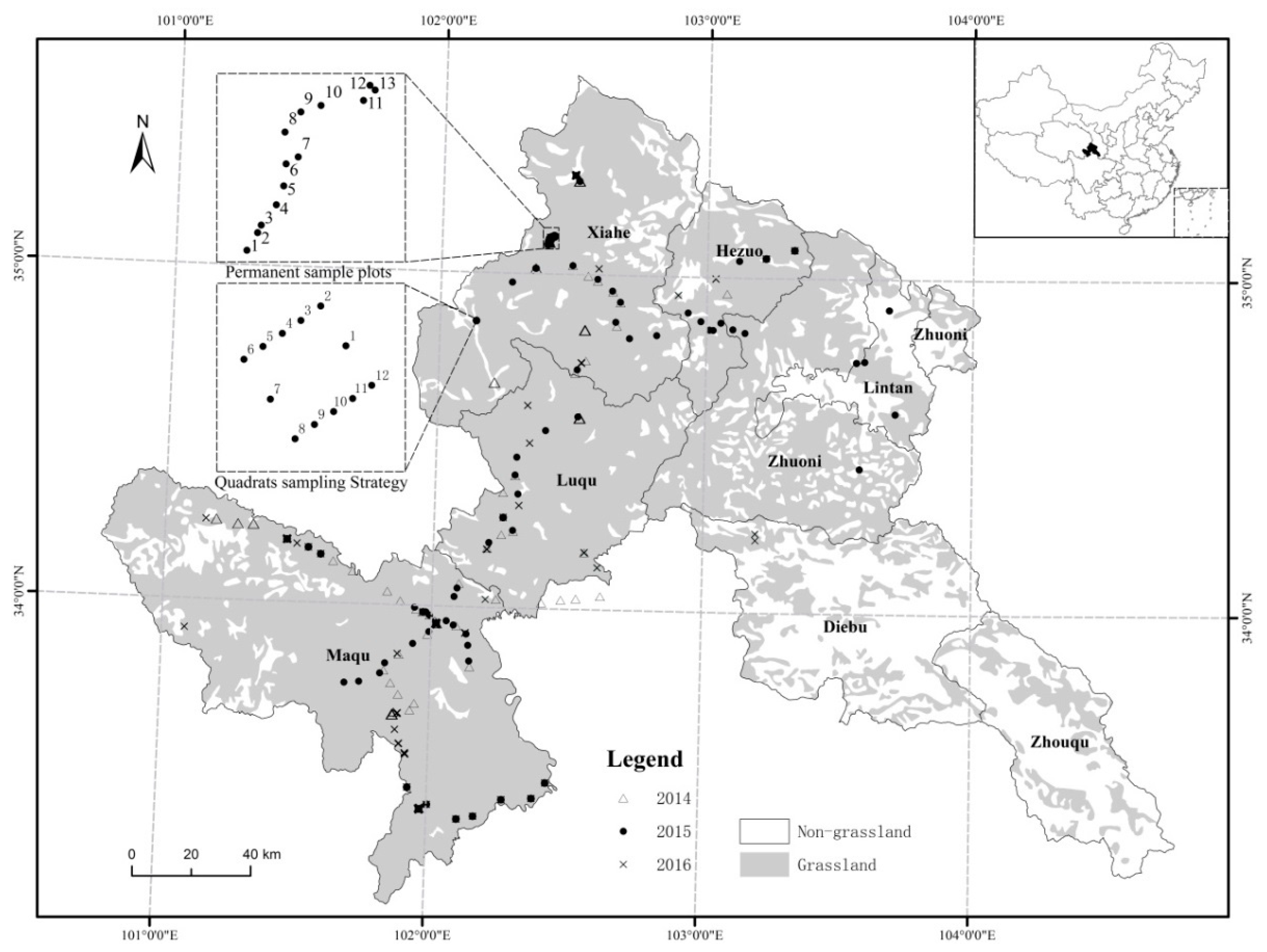
2.1. Study Area
2.2. Sampling Strategy and Data Collection
2.3. Soil, DEM and Meteorological Data
2.4. MODIS Data and Preprocessing
2.5. Construction of Grassland Cover Monitoring Models and Evaluation of Accuracy
2.5.1. Grassland Cover Monitoring Models
2.5.2. Accuracy Evaluation
2.6. Dynamic Variation and Trend Analysis
3. Results and Analysis
3.1. Statistical Analysis of Observed Grassland Cover and Corresponding MODIS Vegetation Indices
3.2. Parametric Model Construction (Linear and Nonlinear) and Precision Evaluation
3.2.1. Single-factor Parametric Model
3.2.2. Multi-factor Parametric Model and Precision Evaluation
3.3. Multi-Factor Non-Parametric Regression Models Based on BP-ANN, SVM and RF and Evaluation of Precision
3.4. Comparison of Stability between Parametric and Non-Parametric Models (Optimum Inversion Model Selection)
3.5. Spatial and Temporal Dynamic Changes in Grassland Cover in Gannan Prefecture
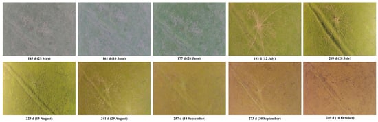
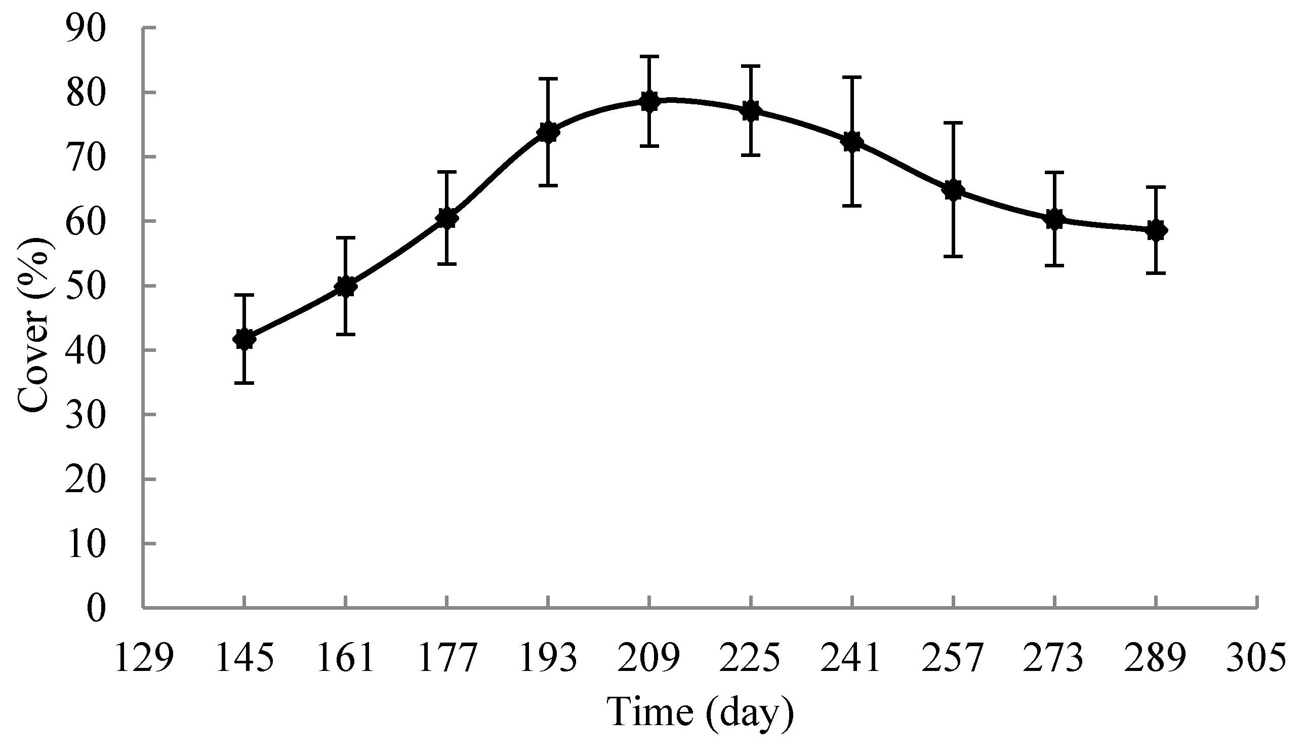
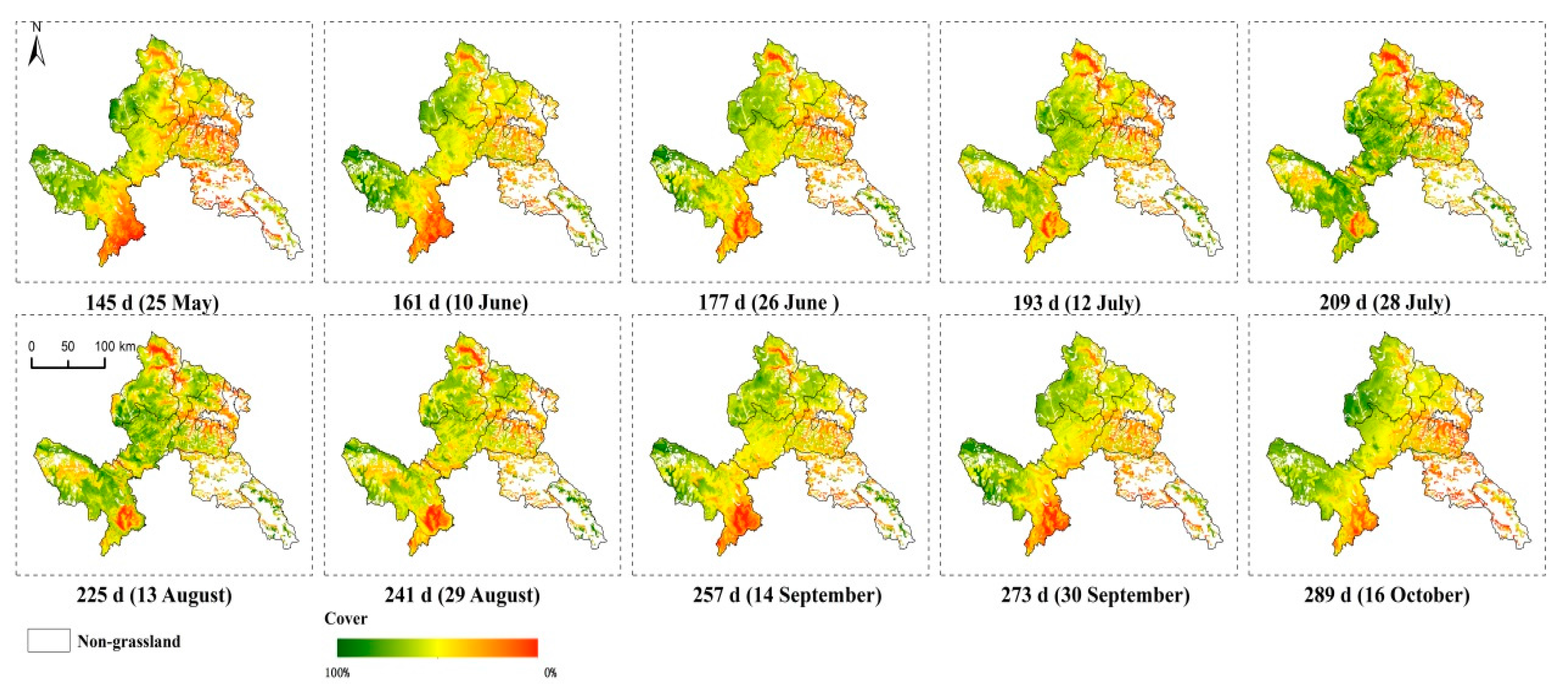
3.5.1. Dynamic Changes During the Growth Season Every 16 day from 2000 to 2016
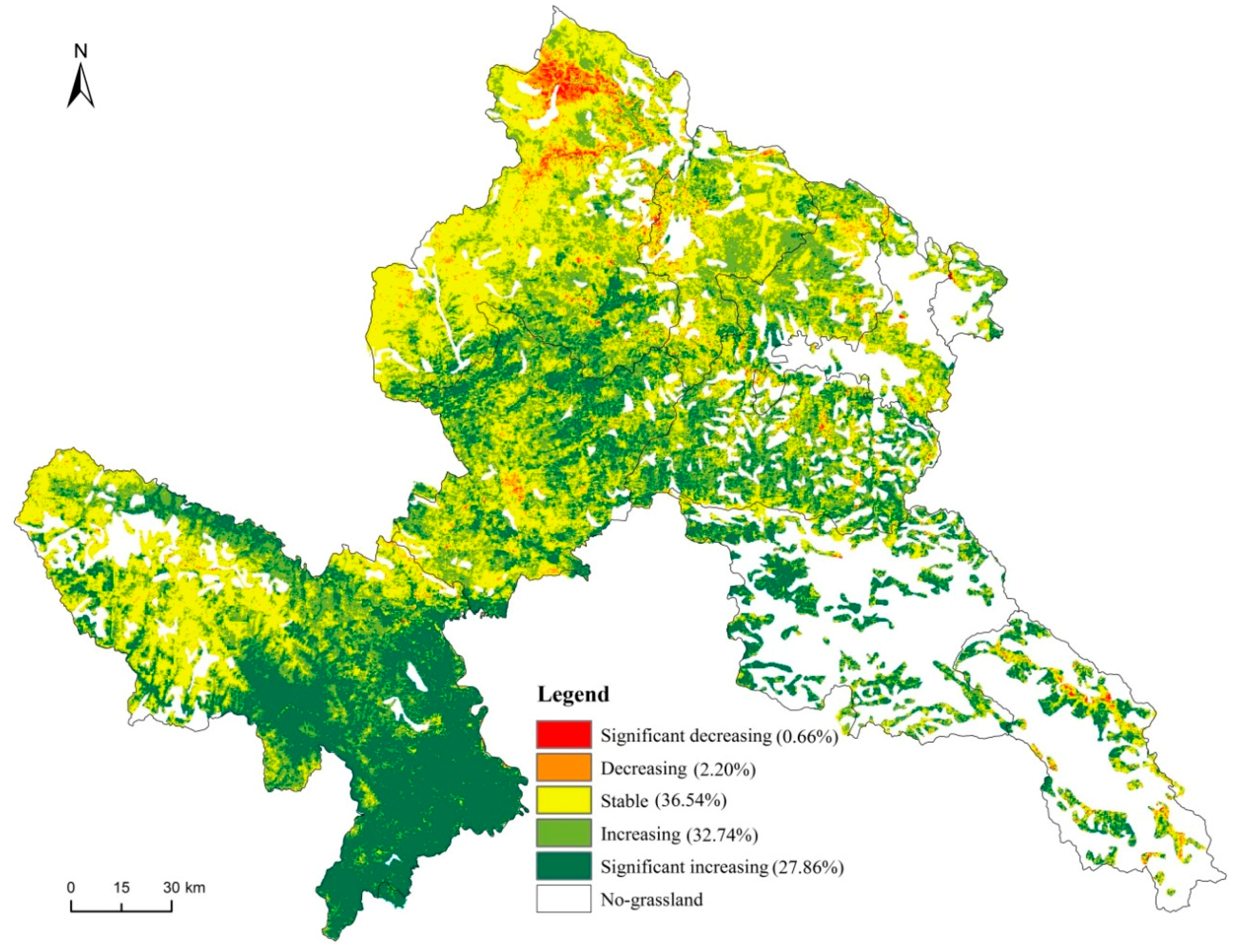
3.5.2. Dynamic Changes in Annual Maximum Grassland Cover
4. Discussion
4.1. Influence of Various Factors on Grassland Cover in Gannan Prefecture
4.2. Comparative Analysis between Multi-Factor Parametric and Non-Parametric Models
4.3. Limitations and Prospects of a Model for Grassland Cover Monitoring in the Study Area
4.3.1. Uncertainties in the Measured Data
4.3.2. Temporal Matching Between Ground Sampling Sites and Remote-Sensing Data
4.3.3. Limitations of the Optimum Estimation Model
5. Conclusions
Acknowledgments
Author Contributions
Conflicts of Interest
References
- Lehnert, L.W.; Meyer, H.; Wang, Y.; Miehe, G.; Thies, B.; Reudenbach, C.; Bendix, J. Retrieval of grassland plant coverage on the Tibetan Plateau based on a multi-scale, multi-sensor and multi-method approach. Remote Sens. Environ. 2015, 164, 197–207. [Google Scholar] [CrossRef]
- Liang, T.; Yang, S.; Feng, Q.; Liu, B.; Zhang, R.; Huang, X.; Xie, H. Multi-factor modeling of above-ground biomass in alpine grassland: A case study in the Three-River Headwaters Region, China. Remote Sens. Environ. 2016, 186, 164–172. [Google Scholar] [CrossRef]
- Yang, S.; Feng, Q.; Liang, T.; Liu, B.; Zhang, W.; Xie, H. Modeling grassland above-ground biomass based on artificial neural network and remote sensing in the three-river headwaters region. Remote Sens. Environ. 2017, 204, 448–455. [Google Scholar] [CrossRef]
- Meng, B.; Ge, J.; Liang, T.; Yang, S.; Gao, J.; Feng, Q.; Cui, X.; Huang, X.; Xie, H. Evaluation of Remote Sensing Inversion Error for the Above-Ground Biomass of Alpine Meadow Grassland Based on Multi-Source Satellite Data. Remote Sens. 2017, 9, 372. [Google Scholar] [CrossRef]
- Qin, X.; Sun, J.; Wang, X. Plant coverage is more sensitive than species diversity in indicating the dynamics of the above-ground biomass along a precipitation gradient on the Tibetan Plateau. Ecol. Indic. 2018, 84, 507–514. [Google Scholar] [CrossRef]
- Feng, H.; Zou, B.; Luo, J. Coverage-dependent amplifiers of vegetation change on global water cycle dynamics. J. Hydrol. 2017, 550, 220–229. [Google Scholar] [CrossRef]
- Hu, J.; Su, Y.; Tan, B.; Huang, D.; Yang, W.; Schull, M.; Bull, M.A.; Martonchik, J.V.; Diner, D.J.; Knyazikhin, Y.; Myneni, R.B. Analysis of the MISR LAI/FPAR product for spatial and temporal coverage, accuracy and consistency. Remote Sens. Environ. 2007, 107, 334–347. [Google Scholar] [CrossRef]
- Dong, Y.; Lei, T.; Li, S.; Yuan, C.; Zhou, S.; Yang, X. Effects of rye grass coverage on soil loss from loess slopes. Int. Soil Water Conserv. Res. 2015, 3, 170–182. [Google Scholar] [CrossRef]
- Hou, J.; Wang, H.; Fu, B.; Zhu, L.; Wang, Y.; Li, Z. Effects of plant diversity on soil erosion for different vegetation patterns. Catena 2016, 147, 632–637. [Google Scholar] [CrossRef]
- Yao, X.; Yu, J.; Jiang, H.; Sun, W.; Li, Z. Roles of soil erodibility, rainfall erosivity and land use in affecting soil erosion at the basin scale. Agric. Water Manag. 2016, 174, 82–92. [Google Scholar] [CrossRef]
- Gao, J.; Liu, Y.S. Determination of land degradation causes in tongyu county, northeast china via land cover change detection. Int. J. Appl. Earth Obs. Geoinf. 2010, 12, 9–16. [Google Scholar] [CrossRef]
- Wang, P.; Deng, X.; Jiang, S. Diffused impact of grassland degradation over space: A case study in Qinghai province. Phys. Chem. Earth-Parts A/B/C 2017, 101, 166–171. [Google Scholar] [CrossRef]
- Guo, S.M. Research of Vegetation Coverage Distribution Changes of Alpine Grassland Based on 3s Technology. Master’s Thesis, Lanzhu University, Lanzhou, China, 2009. [Google Scholar]
- Yi, S.; Zhou, Z.; Ren, S.; Xu, M.; Qin, Y.; Chen, S.; Ye, B. Effects of permafrost degradation on alpine grassland in a semi-arid basin on the Qinghai–Tibetan Plateau. Environ. Res. Lett. 2011, 6, 045403. [Google Scholar] [CrossRef]
- Purevdorj, T.S.; Tateishi, R.; Ishiyama, T.; Honda, Y. Relationships between percent vegetation cover and vegetation indices. Int. J. Remote Sens. 1998, 19, 3519–3535. [Google Scholar] [CrossRef]
- Chen, J.; Yi, S.; Qin, Y.; Wang, X. Improving estimates of fractional vegetation cover based on UAV in alpine grassland on the Qinghai–Tibetan Plateau. Int. J. Remote Sens. 2016, 37, 1922–1936. [Google Scholar] [CrossRef]
- Maresma, Á.; Ariza, M.; Martínez, E.; Lloveras, J.; Martínez-Casasnovas, J. Analysis of Vegetation Indices to Determine Nitrogen Application and Yield Prediction in Maize (Zea mays L.) from a Standard UAV Service. Remote Sens. 2016, 8, 973. [Google Scholar] [CrossRef]
- Holman, F.; Riche, A.; Michalski, A.; Castle, M.; Wooster, M.; Hawkesford, M. High Throughput Field Phenotyping of Wheat Plant Height and Growth Rate in Field Plot Trials Using UAV Based Remote Sensing. Remote Sens. 2016, 8, 1031. [Google Scholar] [CrossRef]
- Yi, S.; Chen, J.; Qin, Y.; Xu, G. The burying and grazing effects of plateau pika on alpine grassland are small: A pilot study in a semiarid basin on the Qinghai-Tibet Plateau. Biogeosciences 2016, 13, 6273–6284. [Google Scholar] [CrossRef]
- Chen, J.; Yi, S.; Qin, Y. The contribution of plateau pika disturbance and erosion on patchy alpine grassland soil on the Qinghai-Tibetan Plateau: Implications for grassland restoration. Geoderma 2017, 297, 1–9. [Google Scholar] [CrossRef]
- Xu, B.; Yang, X.; Tao, W.; Qin, Z.; Liu, H.; Miao, J. Remote sensing monitoring upon the grass production in China. Acta Ecol. Sin. 2007, 27, 405–413. [Google Scholar] [CrossRef]
- Göttlicher, D.; Obregón, A.; Homeier, J.; Rollenbeck, R.; Nauss, T.; Bendix, J. Land-cover classification in the andes of southern ecuador using landsat etm+ data as a basis for svat modelling. Int. J. Remote Sens. 2009, 30, 1867–1886. [Google Scholar] [CrossRef]
- Li, T.; Li, X.; Li, F. Estimating Fractional Cover of Photosynthetic Vegetation and Non-photosynthetic Vegetation in the Xilingol Steppe Region with EO-1 Hyperion Data. Shengtai Xuebao/Acta Ecol. Sin. 2015, 35, 3643–3652. [Google Scholar]
- Li, F.; Jiang, L.; Wang, X.; Zhang, X.; Zheng, J.; Zhao, Q. Estimating grassland aboveground biomass using multitemporal MODIS data in the West Songnen Plain, China. J. Appl. Remote Sens. 2013, 7, 073546. [Google Scholar] [CrossRef]
- Diouf, A.A.; Hiernaux, P.; Brandt, M.; Faye, G.; Djaby, B.; Diop, M.B.; Ndione, J.A.; Tvchon, B. Do Agrometeorological Data Improve Optical Satellite-Based Estimations of the Herbaceous Yield in Sahelian Semi-Arid Ecosystems? Remote Sens. 2016, 8, 668. [Google Scholar] [CrossRef]
- Yue, M.; Wei, F.Z. Based on energy evaluation for agricultural ecological system of Gannan Tibetan autonomous prefecture. Res. Agric. Mod. 2009, 30, 95–97. [Google Scholar]
- Guo, Z.G.; Gao, X.H.; Liu, X.Y.; Liang, T.G. Ecological economic value and functions and classification management for grassland in Gannan prefecture, Gansu province. J. Mt. Sci. 2004, 22, 655–660. [Google Scholar]
- Yang, Q.; Shi, H.M.; Ma, D.L.; Zhang, H.B.; Wen, G.Z.; Mu, Y.J.; Nian, M.X.; Zhao, J.; Bao, F.G. Observation on the adaptability of China grassland red cattle in southern Gansu area. China Cattle Sci. 2007, 33, 25–28. [Google Scholar]
- Zhang, R.; Zhao, X.Y.; Zhao, H.L. Researching on the synthesis competitiveness in the high cold pasturing area—A case of Gannan Autonomy state. J. Northwest Norm. Uni. 2008, 44, 92–97. [Google Scholar]
- Ren, S.L.; Shu-Hua, Y.I.; Chen, J.J.; Qin, Y.; Wang, X.Y. Comparisons of alpine grassland fractional vegetation cover estimation using different digital cameras and different image analysis methods. Pratacult. Sci. 2014, 31, 1007–1013. [Google Scholar]
- Yi, S. FragMAP: A tool for long-term and cooperative monitoring and analysis of small-scale habitat fragmentation using an unmanned aerial vehicle. Int. J. Remote Sens. 2017, 38, 2686–2697. [Google Scholar] [CrossRef]
- Wei, S.G.; Dai, Y.J.; Liu, B.Y.; Ye, A.Z.; Yuan, H. A soil particle-size distribution dataset for regional land and climate modelling in China. Geoderma 2012, 171–172, 85–91. [Google Scholar]
- Zhang, R.; Liang, T.; Feng, Q.; Huang, X.; Wang, W.; Xie, H.; Guo, J. Evaluation and Adjustment of the AMSR2 Snow Depth Algorithm for the Northern Xinjiang Region, China. IEEE J. Sel. Top. Appl. Earth Obs. Remote Sens. 2017, 10, 3892–3903. [Google Scholar] [CrossRef]
- McKenney, D.W.; Pedlar, J.H.; Papadopol, P.; Hutchinson, M.F. The development of 1901–2000 historical monthly climate models for Canada and the United States. Agric. For. Meteorol. 2006, 138, 69–81. [Google Scholar] [CrossRef]
- Bao, Y.; Song, G.; Li, Z.; Gao, J.; Lü, H.; Wang, H.; Cheng, Y.; Xu, T. Study on the spatial differences and its time lag effect on climatic factors of the vegetation in the Longitudinal Range-Gorge Region. Chin. Sci. Bull. 2007, 52, 42–49. [Google Scholar] [CrossRef]
- Zhou, W.; Gang, C.; Chen, Y.; Mu, S.; Sun, Z.; Li, J. Grassland coverage inter-annual variation and its coupling relation with hydrothermal factors in China during 1982–2010. J. Geogr. Sci. 2014, 24, 593–611. [Google Scholar] [CrossRef]
- Yuan, H.; Yang, G.; Li, C.; Wang, Y.; Liu, J.; Yu, H.; Feng, H.; Xu, B.; Zhao, X.; Yang, X. Retrieving Soybean Leaf Area Index from Unmanned Aerial Vehicle Hyperspectral Remote Sensing: Analysis of RF, ANN, and SVM Regression Models. Remote Sens. 2017, 9, 309. [Google Scholar] [CrossRef]
- He, Q. Neural Network and its Application in IR; Graduate School of Library and Information Science, University of Illinois at Urbana-Champaign Spring: Champaign, IL, USA, 1999. [Google Scholar]
- Tiryaki, S.; Aydın, A. An artificial neural network model for predicting compression strength of heat treated woods and comparison with a multiple linear regression model. Constr. Build. Mater. 2014, 62, 102–108. [Google Scholar] [CrossRef]
- Verrelst, J.; Camps-Valls, G.; Muñoz-Marí, J.; Rivera, J.P.; Veroustraete, F.; Clevers, J.G.P.W.; Moreno, J. Optical remote sensing and the retrieval of terrestrial vegetation bio-geophysical properties—A review. ISPRS J. Photogramm. Remote Sens. 2015, 108, 273–290. [Google Scholar] [CrossRef]
- Vapnik, V.; Golowich, S.E.; Smola, A. Support vector method for function approximation, regression estimation, and signal processing. Adv. Neur. Inf. Process. Syst. 1997, 9, 281–287. [Google Scholar]
- Chang, C.C.; Lin, C.J. LIBSVM: A Library For Support Vector Machines; ACM: New York, NY, USA, 2011. [Google Scholar]
- Breiman, L. Random forests. Mach. Learn. 2001, 45, 5–32. [Google Scholar] [CrossRef]
- Han, Z.Y.; Zhu, X.C.; Fang, X.Y.; Wang, Z.Y.; Wang, L.; Zhao, G.X.; Jiang, Y.M. Hyperspectral estimation of apple tree canopy LAI based on SVM and RF regression. Spectrosc. Spectr. Anal. 2016, 36, 800–805. [Google Scholar]
- Jung, M.; Reichstein, M.; Margolis, H.A.; Cescatti, A.; Richardson, A.D.; Arain, M.A.; Arneth, A.; Bernhofer, C.; Bonal, D.; Chen, J.; et al. Global patterns of land–atmosphere fluxes of carbon dioxide, latent heat, and sensible heat derived from eddy covariance, satellite, and meteorological observations. J. Geophys. Res. Biogeol. 2011, 116, 245–255. [Google Scholar] [CrossRef]
- Liu, Y.; Bi, J.W.; Fan, Z.P. Multi-class sentiment classification: The experimental comparisons of feature selection and machine learning algorithms. Expert Syst. Appl. 2017, 80, 323–339. [Google Scholar] [CrossRef]
- Chou, J.S.; Pham, A.D. Nature-inspired metaheuristic optimization in least squares support vector regression for obtaining bridge scour information. Inf. Sci. 2017, 399, 64–80. [Google Scholar] [CrossRef]
- Huang, J.C.; Gao, J.F. An ensemble simulation approach for artificial neural network: An example from chlorophyll a simulation in Lake Poyang, China. Ecol. Inform. 2017, 37, 52–58. [Google Scholar] [CrossRef]
- Zhou, W.; Yang, H.; Huang, L.; Chen, C.; Lin, X.; Hu, Z.; Li, J. Grassland degradation remote sensing monitoring and driving factors quantitative assessment in China from 1982 to 2010. Ecol. Indic. 2017, 83, 303–313. [Google Scholar] [CrossRef]
- Zhao, H.; Liu, S.; Dong, S.; Su, X.; Wang, X.; Wu, X.; Wu, L.; Zhang, X. Analysis of vegetation change associated with human disturbance using MODIS data on the rangelands of the Qinghai-Tibet Plateau. Rang. J. 2015, 37, 77. [Google Scholar] [CrossRef]
- Dong, J.; Tao, F.; Zhang, G. Trends and variation in vegetation greenness related to geographic controls in middle and eastern Inner Mongolia, China. Environ. Earth Sci. 2010, 62, 245–256. [Google Scholar] [CrossRef]
- Ali, I.; Cawkwell, F.; Dwyer, E.; Barrett, B.; Green, S. Satellite remote sensing of grasslands: From observation to management—A review. J. Plant Ecol. 2016, 9, 649–671. [Google Scholar] [CrossRef]
- Li, Z.Q.; Guo, X.L. Topographic effects on vegetation biomass in semiarid mixed grassland under climate change using avhrr ndvi data. Br. J. Environ. Clim. Chang. 2014, 4, 229–242. [Google Scholar] [CrossRef] [PubMed]
- Dodd, M.B.; Lauenroth, W.K.; Burke, I.C.; Chapman, P.L. Association between vegetation patterns and soil texture in the shortgrass steppe. Plant Ecol. 2002, 158, 127–137. [Google Scholar] [CrossRef]
- Fang, J.; Yang, Y.; Ma, W.; Mohammat, A.; Shen, H. Ecosystem carbon stocks and their changes in China’s grasslands. Sci. China Life Sci. 2010, 53, 757–765. [Google Scholar] [CrossRef] [PubMed]
- Piao, S.; Fang, J.; Zhou, L.; Tan, K.; Tao, S. Changes in biomass carbon stocks in China’s grasslands between 1982 and 1999. Glob. Biogeochem. Cycl. 2007, 21. [Google Scholar] [CrossRef]
- Gao, T.; Yang, X.; Jin, Y.; Ma, H.; Li, J.; Yu, H.; Yu, Q.; Zheng, X.; Xu, B. Spatio-temporal variation in vegetation biomass and its relationships with climate factors in the Xilingol grasslands, Northern China. PLoS ONE 2013, 8, e83824. [Google Scholar] [CrossRef] [PubMed]
- Yang, Y.H.; Piao, S.-L. Variations in grassland vegetation cover in relation to climatic factors on the tibetan plateau. J. Plant Ecol. 2006, 30, 1–8. [Google Scholar]
- Cui, X.; Guo, Z.G.; Liang, T.G.; Shen, Y.Y.; Liu, X.Y.; Liu, Y. Classification management for grassland using MODIS data: A case study in the Gannan region, China. Int. J. Remote Sens. 2012, 33, 3156–3175. [Google Scholar] [CrossRef]
- Ma, L.Y. Spatio-temporal dynamic changes of grassland vegetation cover and phenologg in Gannan prefecture. Master’s Thesis, Lanzhu University, Lanzhou, China, 2013. [Google Scholar]
- Feng, Y.; Cui, N.; Gong, D.; Zhang, Q.; Zhao, L. Evaluation of random forests and generalized regression neural networks for daily reference evapotranspiration modelling. Agric. Water Manag. 2017, 193, 163–173. [Google Scholar] [CrossRef]
- Gao, T.; Xu, B.; Yang, X.; Jin, Y.; Ma, H.; Li, J.; Yu, H. Using MODIS time series data to estimate aboveground biomass and its spatio-temporal variation in Inner Mongolia’s grassland between 2001 and 2011. Int. J. Remote Sens. 2013, 34, 7796–7810. [Google Scholar] [CrossRef]
- Deo, R.C.; Sahin, M. Forecasting long-term global solar radiation with an ANN algorithm coupled with satellite-derived (MODIS) land surface temperature (LST) for regional locations in Queensland. Renew. Sust. Energy Rev. 2017, 72, 828–848. [Google Scholar] [CrossRef]
- Yuan, X.L.; Li, L.H.; Tian, X.; Luo, G.P.; Chen, X. Estimation of above-ground biomass using MODIS satellite imagery of multiple land-cover types in China. Remote Sens. Lett. 2016, 7, 1141–1149. [Google Scholar] [CrossRef]
- Eisfelder, C.; Kuenzer, C.; Dech, S. Derivation of biomass information for semi-arid areas using remote-sensing data. Int. J. Remote Sens. 2012, 33, 2937–2984. [Google Scholar] [CrossRef]


| Time Period | 1-th | 2-th | 3-th | … | i-th | … | n-th |
|---|---|---|---|---|---|---|---|
| 1-th | 0 | 0~1 | 0~2 | … | 0~i − 1 | … | 0~n − 1 |
| 2-th | 1 | 1~2 | … | 1~i − 1 | … | 1~n − 1 | |
| 3-th | 2 | … | 2~i − 1 | … | 2~n − 1 | ||
| … | … | 3~i − 1 | … | 3~n − 1 | |||
| i-th | … | … | ...~n − 1 | ||||
| … | … | n − 2~n − 1 | |||||
| n-th | n − 1 |
| Index | Statistical Indicator | Study Area | |||||||
|---|---|---|---|---|---|---|---|---|---|
| Zhuoni | Xiahe | Maqu | Lintan | Luqu | Hezuo | Diebu | All | ||
| NDVI | Maximum | 0.71 | 0.86 | 0.85 | 0.76 | 0.85 | 0.80 | 0.75 | 0.86 |
| Minimum | 0.62 | 0.28 | 0.43 | 0.68 | 0.56 | 0.45 | 0.52 | 0.28 | |
| Average | 0.67 | 0.62 | 0.76 | 0.72 | 0.72 | 0.66 | 0.63 | 0.67 | |
| Standard deviation | 0.05 | 0.14 | 0.08 | 0.04 | 0.08 | 0.12 | 0.16 | 0.14 | |
| CV | 0.07 | 0.22 | 0.11 | 0.06 | 0.11 | 0.19 | 0.25 | 0.20 | |
| EVI | Maximum | 0.51 | 0.68 | 0.76 | 0.57 | 0.70 | 0.64 | 0.48 | 0.76 |
| Minimum | 0.38 | 0.14 | 0.28 | 0.48 | 0.34 | 0.25 | 0.36 | 0.14 | |
| Average | 0.44 | 0.40 | 0.58 | 0.51 | 0.52 | 0.47 | 0.42 | 0.47 | |
| Standard deviation | 0.06 | 0.12 | 0.10 | 0.05 | 0.10 | 0.15 | 0.09 | 0.14 | |
| CV | 0.13 | 0.31 | 0.18 | 0.09 | 0.19 | 0.31 | 0.20 | 0.30 | |
| Cover | Maximum | 94.75 | 99.83 | 99.87 | 91.31 | 98.01 | 96.28 | 85.64 | 99.87 |
| Minimum | 33.07 | 1.38 | 18.66 | 58.43 | 33.01 | 26.72 | 67.52 | 1.38 | |
| Average | 58.37 | 63.36 | 83.83 | 78.61 | 75.49 | 67.12 | 66.58 | 70.62 | |
| Standard deviation | 27.39 | 27.67 | 17.98 | 17.67 | 18.87 | 25.89 | 12.81 | 25.99 | |
| CV | 0.47 | 0.44 | 0.21 | 0.22 | 0.25 | 0.39 | 0.17 | 0.37 | |
| Variable | Linear | Exponential | Logarithm | Power | ||||
|---|---|---|---|---|---|---|---|---|
| R2 | RMSE | R2 | RMSE | R2 | RMSE | R2 | RMSE | |
| EVI | 0.49 | 17.39 | 0.46 | 17.06 | 0.52 | 16.96 | 0.50 | 17.37 |
| NDVI | 0.47 | 17.73 | 0.46 | 17.96 | 0.47 | 17.81 | 0.47 | 17.77 |
| P | 0.39 | 19.08 | 0.37 | 19.60 | 0.41 | 18.76 | 0.40 | 18.94 |
| T | 0.31 | 20.93 | 0.28 | 21.40 | 0.33 | 20.55 | 0.31 | 20.97 |
| X | 0.05 | 24.11 | 0.05 | 24.07 | 0.05 | 24.10 | 0.05 | 24.06 |
| H | 0.06 | 24.18 | 0.06 | 24.18 | 0.06 | 24.18 | 0.06 | 24.18 |
| Y | 0.05 | 24.16 | 0.05 | 24.15 | 0.05 | 24.16 | 0.05 | 24.14 |
| C1 | 0.03 | 24.26 | 0.03 | 24.24 | 0.03 | 24.25 | 0.03 | 24.25 |
| S2 | 0.05 | 24.20 | 0.05 | 24.20 | 0.05 | 24.19 | 0.05 | 24.19 |
| S | 0.03 | 24.37 | 0.03 | 24.37 | - | - | - | - |
| C2 | 0.03 | 24.44 | 0.03 | 24.44 | 0.04 | 24.41 | 0.04 | 24.40 |
| TPI | 0.01 | 24.45 | 0.01 | 24.45 | 0.01 | 24.46 | 0.01 | 24.46 |
| S1 | 0.02 | 24.46 | 0.02 | 24.46 | 0.02 | 24.48 | 0.02 | 24.48 |
| A | 0.02 | 24.47 | 0.02 | 24.47 | - | - | - | - |
| Vegetation Index | Parameter Estimation and T Test | Regression Significance Test | |||
|---|---|---|---|---|---|
| Parameter | Estimated Value | T | R2 | F | |
| EVI | A | 0.137 | 15.744 ** | 0.49 | 247.878 ** |
| B | −0.096 | 2.663 ** | |||
| NDVI | A | 0.003 | 18.739 ** | 0.47 | 351.158 ** |
| B | 0.470 | 39.395 ** | |||
| P | A | 543.286 | 13.886 ** | 0.33 | 192.829 ** |
| B | −420.647 | −2.577 * | |||
| TAs | A | 14.912 | 10.317 ** | 0.21 | 106.449 ** |
| B | 48.217 | 7.996 ** | |||
| X | A | −0.001 | −3.042 * | 0.02 | 9.307 * |
| B | 102.771 | 698.162 ** | |||
| H | A | 4.447 × 10⁻⁴ | 3.506 ** | 0.03 | 12.292 ** |
| B | 3175.107 | 107.046 ** | |||
| Y | A | −0.004 | −2.568 * | 0.02 | 6.596 * |
| B | 35.147 | 149.540 ** | |||
| C1 | A | −0.001 | −2.891 ** | 0.02 | 8.361 * |
| B | 17.914 | 32.479 ** | |||
| S2 | A | 1.236 | 2.086 * | 0.01 | 4.352 * |
| B | 24.142 | 9.769 ** | |||
| S | A | −0.011 | 1.801 | 0.01 | 3.245 |
| B | 2.956 | 6.526 ** | |||
| C2 | A | −0.03 | −1.285 | 1.644 × 10⁻³ | 1.652 |
| B | 22.334 | 9.628 ** | |||
| S1 | A | 0.004 | 0.324 | 2.658 × 10⁻⁴ | 0.105 |
| B | 31.515 | 39.366 ** | |||
| T | A | −4.889 × 10⁻⁴ | −0.281 | 1.993 × 10⁻⁴ | 0.079 |
| B | 4.104 | 31.991 ** | |||
| A | A | −0.006 | −0.027 | 1.865 × 10⁻⁶ | 0.001 |
| B | 144.943 | 9.364 ** | |||
| Variable | Formula | R2 |
|---|---|---|
| EVI | y = 0.137ln(x) − 0.096 | 0.49 |
| NDVI | y = 0.003x + 0.470 | 0.47 |
| P | y = 543.286ln(x) − 420.647 | 0.33 |
| T | y = 14.912ln(x) + 48.217 | 0.21 |
| X | y = −0.001x102.770 | 0.02 |
| H | y = 4.447×10⁻⁴e 3175.107x | 0.03 |
| Y | y = −0.004x35.147 | 0.02 |
| C1 | y = −0.001e17.914x | 0.04 |
| S2 | y = 1.236ln(x) + 24.142 | 0.01 |
| Model Forms | Training Set | Test Set | ||
|---|---|---|---|---|
| R2 | RMSE | R2 | RMSE | |
| Linear | 0.62 | 15.014 | 0.60 | 15.39 |
| Logarithm | 0.63 | 14.885 | 0.61 | 15.12 |
| Power | 0.60 | 15.523 | 0.58 | 15.70 |
| Reciprocal | 0.61 | 15.378 | 0.59 | 15.52 |
| Model Forms | Formula | R2 | F |
|---|---|---|---|
| Linear | y = 361.0690 + 0.0247P − 0.1398T − 0.0648S2 − 0.0261H − 0.3031C1 − 6.7056X + 11.3646Y + 102.9434EVI + 23.7885NDVI | 0.62 | 71.01 ** |
| Logarithm | y = 2877.5978 + 36.8336ln(P) − 12.7674ln(T) + 1.5335ln(S2) − 98.8390ln(H) − 2.3321ln(C1) − 700.1303ln(X) + 299.7008ln(Y) + 53.6374ln(EVI) + 2.0236ln(NDVI) | 0.63 | 73.04 ** |
| Power | y = 1.3840P0.5411T−0.1455S20.0523H−1.0555C10.0072X−0.8194Y3.7514EVI0.6908NDVI0.2119 | 0.60 | 58.99 ** |
| Reciprocal | y = −406.7349 − 2.9639 × 10⁴/P − 1.7307 × 10³/T − 147.3110/S2 + 1.7582 × 10⁵/H + 21.8384/C1 + 7.0831 × 10⁴/X − 6.2091 × 10³/Y − 17.1820/EVI − 8.4375/NDVI | 0.60 | 65.75 ** |
| Method | Training Set | Test Set | ||
|---|---|---|---|---|
| R2 | RMSE | R2 | RMSE | |
| BP-ANN | 0.83 | 10.288 | 0.72 | 13.38 |
| SVM | 0.90 | 7.804 | 0.73 | 12.83 |
| RF | 0.96 | 5.289 | 0.78 | 10.84 |
| Model | Factor | Function | SDR2 | SDRMSE |
|---|---|---|---|---|
| Single factor parametric models (including linear and nonlinear forms) | EVI | Logarithm | 0.182 | 3.205 |
| NDVI | Linear | 0.170 | 2.900 | |
| P | Logarithm | 0.171 | 2.689 | |
| T | Logarithm | 0.143 | 2.394 | |
| X | Power | 0.054 | 1.566 | |
| H | Exponential | 0.074 | 1.478 | |
| Y | Power | 0.062 | 1.595 | |
| C1 | Exponential | 0.039 | 1.666 | |
| S2 | Logarithm | 0.044 | 2.006 | |
| Multi-factor parametric models (including linear and nonlinear forms) | EVI, NDVI, P, T, X, H, Y, C1, S2 | linear | 0.158 | 2.918 |
| Logarithm | 0.171 | 3.263 | ||
| Power | 0.167 | 3.142 | ||
| Reciprocal | 0.184 | 3.520 | ||
| Multi-factor non-parametric models (nonlinear form) | EVI, NDVI, P, T, X, H, Y, C1, S2 | BP-ANN | 0.062 | 1.615 |
| SVM | 0.082 | 1.732 | ||
| RF | 0.095 | 2.354 |
© 2018 by the authors. Licensee MDPI, Basel, Switzerland. This article is an open access article distributed under the terms and conditions of the Creative Commons Attribution (CC BY) license (http://creativecommons.org/licenses/by/4.0/).
Share and Cite
Meng, B.; Gao, J.; Liang, T.; Cui, X.; Ge, J.; Yin, J.; Feng, Q.; Xie, H. Modeling of Alpine Grassland Cover Based on Unmanned Aerial Vehicle Technology and Multi-Factor Methods: A Case Study in the East of Tibetan Plateau, China. Remote Sens. 2018, 10, 320. https://doi.org/10.3390/rs10020320
Meng B, Gao J, Liang T, Cui X, Ge J, Yin J, Feng Q, Xie H. Modeling of Alpine Grassland Cover Based on Unmanned Aerial Vehicle Technology and Multi-Factor Methods: A Case Study in the East of Tibetan Plateau, China. Remote Sensing. 2018; 10(2):320. https://doi.org/10.3390/rs10020320
Chicago/Turabian StyleMeng, Baoping, Jinlong Gao, Tiangang Liang, Xia Cui, Jing Ge, Jianpeng Yin, Qisheng Feng, and Hongjie Xie. 2018. "Modeling of Alpine Grassland Cover Based on Unmanned Aerial Vehicle Technology and Multi-Factor Methods: A Case Study in the East of Tibetan Plateau, China" Remote Sensing 10, no. 2: 320. https://doi.org/10.3390/rs10020320
APA StyleMeng, B., Gao, J., Liang, T., Cui, X., Ge, J., Yin, J., Feng, Q., & Xie, H. (2018). Modeling of Alpine Grassland Cover Based on Unmanned Aerial Vehicle Technology and Multi-Factor Methods: A Case Study in the East of Tibetan Plateau, China. Remote Sensing, 10(2), 320. https://doi.org/10.3390/rs10020320