Article

Early-Season Stand Count Determination in Corn via Integration of Imagery from Unmanned Aerial Systems (UAS) and Supervised Learning Techniques

1
Department of Agronomy, Kansas State University, 2004 Throckmorton Plant Science Center, Manhattan, KS 66506, USA
2
Department of Computer Science, Kansas State University, 2184 Engineering Hall, 1701D Platt St., Manhattan, KS 66506, USA
3
Department of Technology and Development of Corn and Sorghum, Corn Agronomic Modelling; Monsanto Argentina, Pergamino B2700, Argentina
4
Department of Agricultural Economics, Kansas State University, 342Waters Hall, Manhattan, KS 66506, USA
5
Biological and Agricultural Engineering Department, Kansas State University, Seaton Hall, Manhattan, KS 66506, USA
6
PrecisionHawk, 8601 Six Forks Rd #600, Raleigh, NC 27615, USA
*
Author to whom correspondence should be addressed.
Remote Sens. 2018, 10(2), 343; https://doi.org/10.3390/rs10020343
Submission received: 20 January 2018 / Revised: 19 February 2018 / Accepted: 20 February 2018 / Published: 23 February 2018
(This article belongs to the Special Issue Remote Sensing from Unmanned Aerial Vehicles (UAVs))

Abstract

:
Corn (Zea mays L.) is one of the most sensitive crops to planting pattern and early-season uniformity. The most common method to determine number of plants is by visual inspection on the ground but this field activity becomes time-consuming, labor-intensive, biased, and may lead to less profitable decisions by farmers. The objective of this study was to develop a reliable, timely, and unbiased method for counting corn plants based on ultra-high-resolution imagery acquired from unmanned aerial systems (UAS) to automatically scout fields and applied to real field conditions. A ground sampling distance of 2.4 mm was targeted to extract information at a plant-level basis. First, an excess greenness (ExG) index was used to individualized green pixels from the background, then rows and inter-row contours were identified and extracted. A scalable training procedure was implemented using geometric descriptors as inputs of the classifier. Second, a decision tree was implemented and tested using two training modes in each site to expose the workflow to different ground conditions at the time of the aerial data acquisition. Differences in performance were due to training modes and spatial resolutions in the two sites. For an object classification task, an overall accuracy of 0.96, based on the proportion of corrected assessment of corn and non-corn objects, was obtained for local (per-site) classification, and an accuracy of 0.93 was obtained for the combined training modes. For successful model implementation, plants should have between two to three leaves when images are collected (avoiding overlapping between plants). Best workflow performance was reached at 2.4 mm resolution corresponding to 10 m of altitude (lower altitude); higher altitudes were gradually penalized. The latter was coincident with the larger number of detected green objects in the images and the effectiveness of geometry as descriptor for corn plant detection.

Graphical Abstract

1. Introduction

Corn (Zea mays L.) is one of the most responsive grain crops to agronomic management practices including planting pattern and plant density [1,2]. Corn has a limited capacity to compensate for missing plants within a row, consequently penalizing grain yield per unit land area at the end of the season [3,4,5]. One of the most frequent practices to determine the final number of emerged plants is by visual inspection on the ground [6]. This is a labor-intensive, time-demanding, and cumbersome activity for farmers or researchers. Therefore, there is a need to find alternative and novel techniques to quantify plant stands. The novel process should also include quick data processing and data analyses so that the outcomes can help for efficient planning of operations (e.g., re-planting decisions) on the farm [7]. Recent advances in ground sensors and computer vision have provided new insights into plant counting via proximal sensing [8,9]. The proximal sensing method can provide potential applications of automation and mechanization, which substantially reduces the cost of field scouting [10]. Shertha et al. [11] reported the use of the size and shape of corn plants to estimate plant density and row spacing via video frame sequencing, segmentation, and object classification using ground vehicles. In the same context, ground laser line-scanning was adopted to automatically locate stalk and interplant spacing [10]. Ground vehicles are used to mount proximal sensors or cameras to document images and videos. However, the use of ground vehicles is limited to small areas and often dependent on good trafficable conditions to successfully implement a programmed task. To overcome this, implementation and the use of remote sensing using aerial or satellite images and data is gaining importance. Thorp et al. [12] reported the use of aerial hyperspectral data and principal components analysis (PCA) for estimating densities of plants in corn fields. From the same authors, the best performance for the proposed method was reported at the later-vegetative stage (R2 = 0.79) using 6-m resolution imagery. Early-season estimation of plant densities was significantly limited due to the dominant soil background signal when using meter level resolution imagery [12,13].
The use of small unmanned aerial systems (UAS) fills the gap of information between proximal ground sensing and meter spatial resolution platforms. The UAS platforms deliver unprecedented ultra-high spatial resolution imagery and flexible revisit time, and offer high versatility under adverse weather conditions [14,15]. In this context, the use of UAS has been reported in agriculture for crop and weed detection [16,17,18,19]. For weed management, detailed knowledge on the spatial distribution of crops and weeds can significantly reduce the impact of agrochemicals on the environment by using site-specific interventions [17]. Moreover, early detection of crop and weeds aligns with best practices to maximize the effectiveness of agrochemical applications and yield potential [17]. Perez-Ortiz et al. [20] reported the use of a support vector machine (SVM) classifier, utilizing color intensity and geometrical information as input features for weed and crop mapping. The spatial resolution was critical in the performance of the classifier as also identified by Peñaet et al. [16].
In general, the implementation of UAS in agriculture has been focused on the extraction of information at the “canopy scale” for further biophysical and yield prediction [21,22]. This approach has been extensively reported via integration of UAS and sensors: RGB, multi-spectral, hyperspectral, and thermal imagery had been used to estimate biomass [23], LAI [23,24,25,26,27,28], canopy height [21,23,29,30], nitrogen [27,31,32], chlorophyll [32,33], and temperature [34,35,36]. Recently, Jin et al. [37] estimated plant density in wheat from UAS observations using a RGB sensor, ultra-high-resolution imagery, and a support vector machine classifier. Modern approaches on smart farming typically need detailed knowledge of the current status of crops in the fields. The earlier the yield-limiting factors are identified at the field level, the greater the chances to understand the causes and identify potential farming solutions [17]. However, most of the studies on plant density estimation have been implemented via utilization of RGB sensors and computer vision via ground vehicles [8,9,38,39]. Scarce attention has been focused on counting and segmenting individual plants in real field conditions via UAS. Recently, Gnädinger and Schmidhalter [40] implemented a digital counting procedure using a decorrelation stretch contrast enhancement in the RGB feature space domain via UAS. The developed method utilizes the color differences between young and old leaves to estimate plants of different age groups in the image, with an R2 of 0.89 between ground-truthing and estimated plant count. However, the challenge of image thresholding techniques is that they may be prone to misclassification due to the similar spectral response of target and non-target vegetation in the image [41,42].
The current work aims to contribute to the transition from passive and time-delayed workflows into more automatized, reactive, and integrated systems of managing information on monitoring crop performance on farmers’ fields [43,44,45] by developing a tool for quantifying early-season stand counts for corn. Briefly, the present work has been implemented using ultra-high-resolution imagery for plant metric extraction and the workflow was developed by applying the following steps: (i) identify green and non-green regions, (ii) perform a row detection procedure, (iii) extract geometric descriptors of the green objects, and as a last step, (iv) train a decision tree classifier to retrieve information on count and location of the corn plants.

2. Materials and Methods

2.1. Experimental Sites

Two fields were included to test the workflow under different field conditions such as crop residue, soil backscatter, and crop growth stages. Farmers’ fields sites were located in the NE region of Kansas (KS), US (Figure 1). Site 1 was located at Atchison County, KS (39°33′14.84″N, 95°33′46.07″W). Site 2 was located at Jefferson County, KS (39°3′23.60″N, 95°23′19.70″W). Both fields were managed in a soybean-corn rotation. The size of the field in site 1 was 18 hectares, managed under rainfed conditions. The size of the field in site 2 was 64 hectares, under irrigation The plant density in both the fields was 7.5 plants m−2 and inter-row distance 0.75 m.

2.2. Platform, Sensor, and Field Data Collection

A UAS octocopter platform (S1000, DJI, Shenzhen, China) was utilized to collect the aerial images and data. The platform included the A2 flight controller and Global Positioning System (GPS) units used to set up flight missions (S1000, DJI, Shenzhen, China). The flight parameters setting was controlled using UgCs ground station software (UgCs, Riga, Latvia). A PX4 Pixhawk autopilot [46] was installed in the same platform for full control of the intervalometer of the sensor via Mission Planner ground station, an open-source software developed by Michael Osborne (http://planner.ardupilot.com). Nine sample areas of 0.2 hectares were randomly selected and marked in each field prior to the growing season to account for varied spatial conditions from existing residues and non-corn objects. Flights used an automatic setting pattern of 4 parallel lines with a time-lapse of 4 s between images, targeting 25–30 images in each sample region of the field. Sidelapping and overlapping were set to 20%, targeting a consistent distribution of sample images in each sample area. The low overlapping requirement increases the efficiency of the flight and post-processing time compared to other data collection approaches (orthomosaic stitching) to analyze UAS data. The platform, camera orientation, and flight direction were set parallel to the direction of the rows. UAS flight autonomy was set for 15 min; 2 and 3 flights were needed to cover the nine sample areas for sites 1 and 2, respectively
The platform sensor included was an Alpha ILCE A5100 RGB Sony camera (Tokyo, Japan), mounted with a Sony SELP1650 PZ 16-50 mm lens (sensor resolution is 6000 × 4000 pixels). The aperture and exposure time was adjusted manually prior to each mission considering the ground speed of the UAS and light conditions at the time of flights. In all flights, the camera settings used manual exposure control; shutter speed was set to 1/3000 s, aperture to f5, ISO to 400 and 16 mm focal length configuration. One flight in each site was performed between May and June with full sun and 2–3 m s−1 wind conditions (Table 1). On the date of the flights, sites 1 and 2 were at 2 and 2–3 visible leaves growth stage, respectively. Higher soil temperatures and adequate soil moisture conditions during the planting–emergence period in site 2 explained similar growth stages encountered in both locations on the date of the flights, despite a late planting date in site 2. The flight altitude was set to 10 m reaching a spatial resolution of 2.4 mm.

2.3. Data Processing

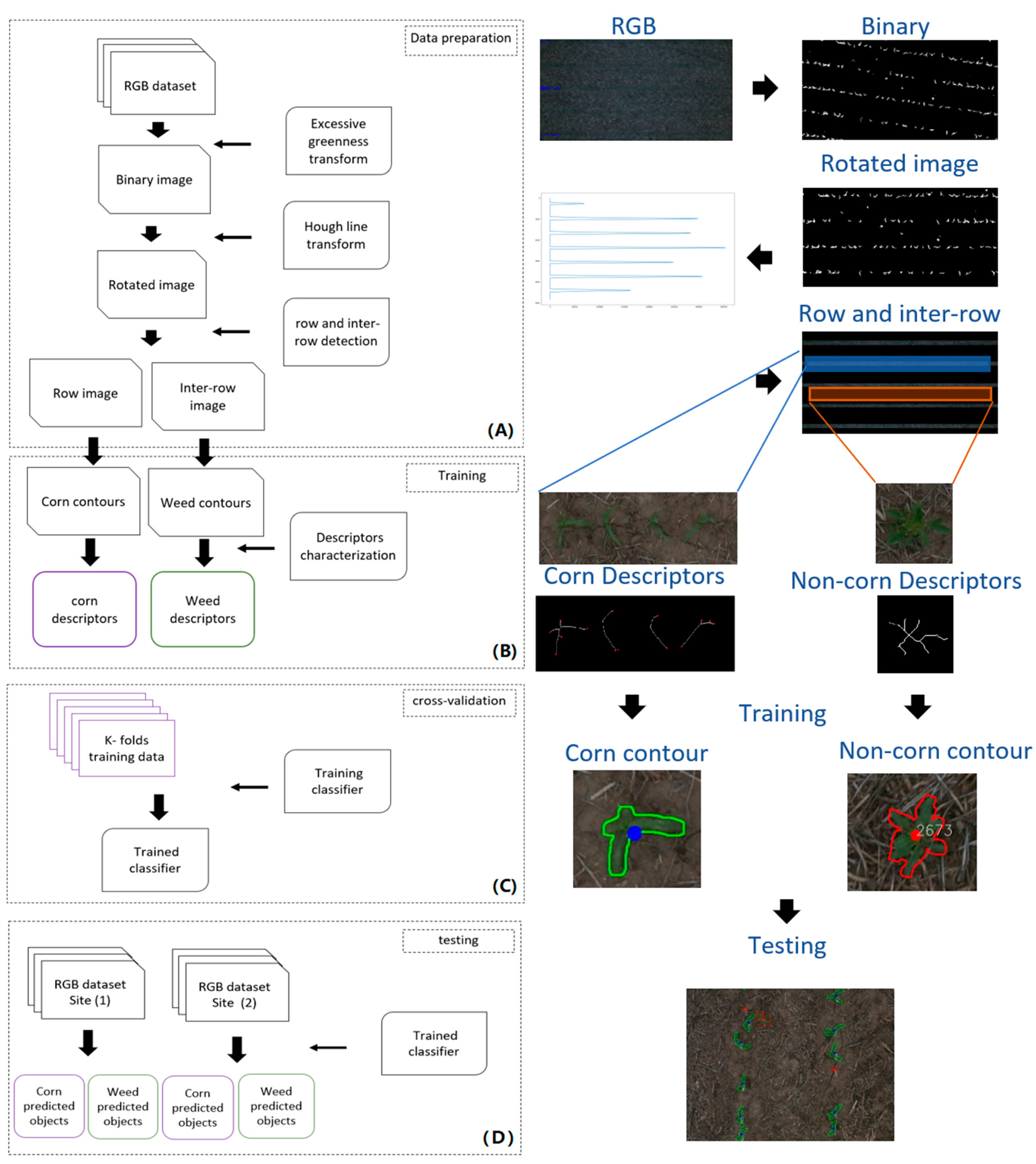
The following workflow including five steps (Figure 2) was developed and implemented after the images were collected from the fields: (1) images were converted into excess greenness (ExG)–vegetation index, (2) row detection and contours were delineated, (3) geometric descriptors were built from contours, (4) classifier training, and (5) classifier testing.
Steps 1, 2, and 3 were implemented via OpenCV Python modules [47], steps 4 and 5 were implemented via Sklearn Python modules [48].
For each site, image data sets were randomly divided into training (60%) and testing (40%) data sets. The training data set was used to predict the value of a target class by learning the decision rules inferred from the geometric descriptors of that class (corn or non-corn objects). The trained decision rules were then evaluated in a new data set (testing) to evaluate the performance of the model exposed to an independent data set.

2.4. Vegetation Detection

In the training data set, the images were first utilized to classify vegetation and background pixels. The excess green index (ExG) [49] helps stretch the contrasting intensity response between green and background pixels. In addition, a bilateral filter was applied to decrease the noise intensity of each channel while preserving the edges of the green objects [41].
ExG = 2 × Green − Red − Blue
A morphological operation was implemented to facilitate the isolation of green contours in the image by computing the corresponding intensity between contours and background. It includes both erosion and dilation transformations by utilizing a predefined kernel size to preserve the integrity of the green objects in the image [41]. An Otsu threshold procedure was adopted to transform the ExG grey scale into a binary image by using a discriminant criterion in the ExG scale. The method automatically finds an optimal threshold value between both green and background classes [50] by minimizing the intra-class variance as much as possible.
σ2w(t) = ω0(t)σ20 (t) + ω1(t)σ21 (t)
ω0 and ω1 are the probabilities of the two classes and σ20 and σ21 are the variances of these two classes. “t” is the desired threshold that minimizes weighted sum of variances of these two classes. The binary transformation assigns a value of 1 to green pixels and 0 to background. Small non-target green contours, <400 connected pixels, are eliminated using a conditional rule.

2.5. Row Detection

First, canny edge detection was implemented to map structures with contrasting ExG intensity in the image. Edges are mostly related to the transitional regions between green objects and background pixels [41]. Hough transformation was adopted to define the orientation angle of the images [51]. The solution to the angle rotation was solved by a voting process of all possible angles between the Hough lines and the reference horizontal axis of the image. The angle that received more votes was chosen as the solution for the entire image rotation.
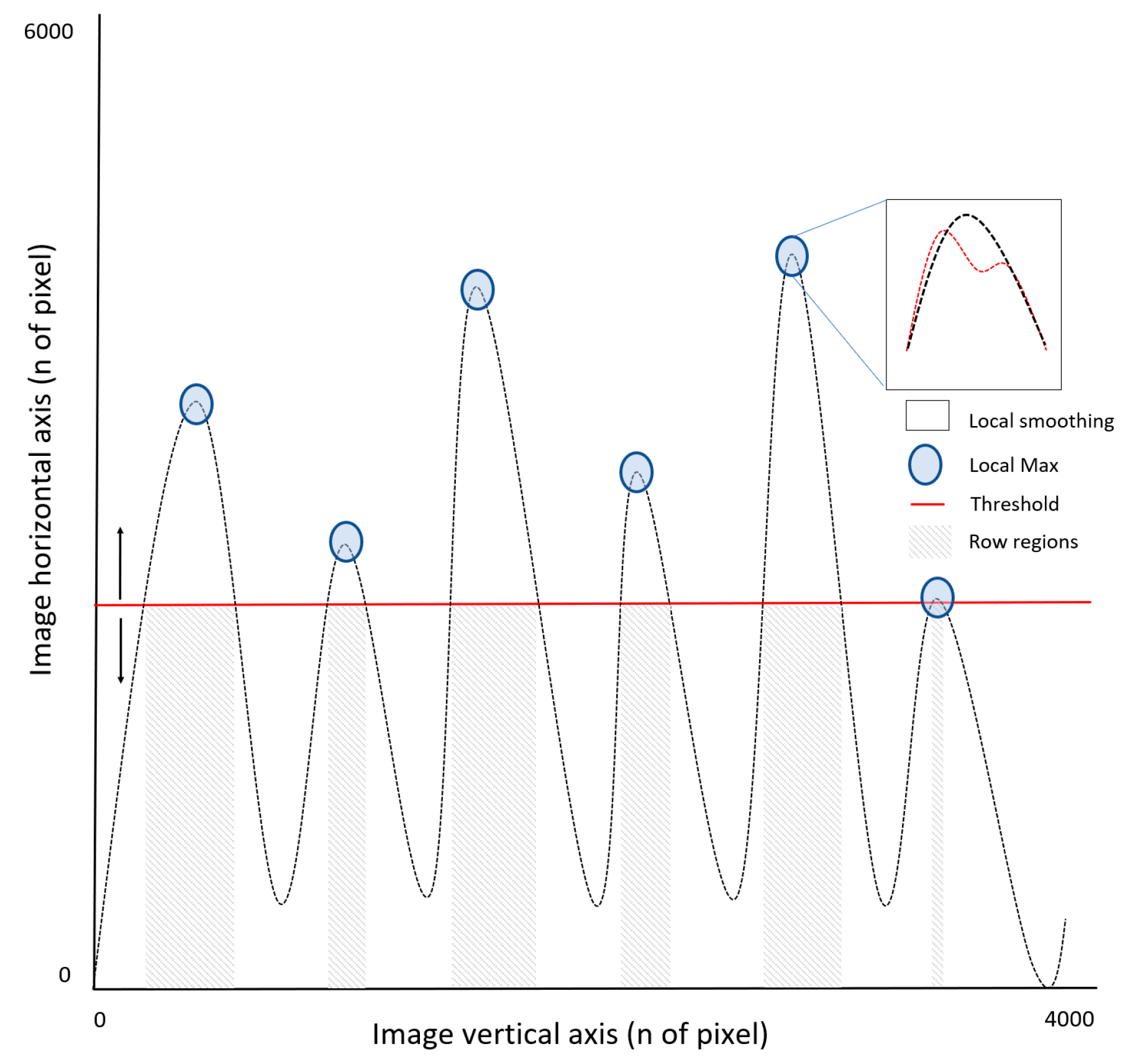
The ExG intensity was projected to the vertical axis of the image. The Savitzky–Golay [42] filter was utilized to smooth local-maxima peaks to better target the candidate areas for rows location (Figure 3). A relative threshold value defines the peaks that define the rows in the vertical projection of the image as follows: each peak must reach one third of the previous one, ExG intensity to be assumed as rows in the vertical axis. The selected peaks represent the rows of the crops in the image. In the same manner, the width of each row was equal to the width of the crest at the thresholding region. The process does not require external user supervision (automated process) to define an optimal threshold to locate the rows, allowing massive scaling of this step.
I A =   { I A i f   I i   I i 1 / 3 I i i f   I i <   I i 1 / 3
I A denotes the threshold that defines whether a peak is a crop row. I i is the sum of intensities of pixels in ith peak. The equation is from i = 2 to n where n is the number of peaks found.

2.6. Feature Descriptors

All contours were extracted from the row and inter-row areas of the image and labeled as corn and non-corn contours, respectively. This approach enables the scaling of the training as no manual tagging of classes is needed. The procedure assumes all contours in the inner region of the row belong to “corn class” and all inter-row contours belong to “non-corn class”. Each contour is characterized by a set of 10 geometric descriptors. This step explores the potential of different geometries to efficiently characterize corn and non-corn objects.
Geometric descriptors were evaluated using the feature importance procedure based on the mean decrease of impurity [52]. Features decreasing the impurity have more importance in the selection, which accounts for potential collinearity between features by penalizing collinear features. According to the feature selection, aspect ratio, axis–diameter ratio, convex area, thinness, and solidity were found as significant contributors to characterize the two types of objects in the training data set.

2.7. Classifier Training

A decision tree (DT) classifier was implemented using the information of the geometric descriptors in each class as input features [53,54]. A 6-fold, cross-validation (CV) procedure was implemented by leaving one out cross validation (LOOCV). It was utilized as a first approach as to how the classifier may generalize to the new independent data set (testing), and to identify potential overfitting of the model [53] (Table 2). The DT was trained to relate the descriptors to the labeled corn and non-corn objects. Due to unbalanced sizes between classes, decision nodes were differently weighed to prevent class overfitting in the classifier. The 6-fold CV was used as an intermediate checkpoint of the classifier performance evaluation. The goal of this step was to create a model that predicts the value of a target class by learning the decision rules inferred from the geometric descriptors of that class. A model-selection procedure was used to determine the DT structure by finding a non-dominated solution representing a trade-off between the classifier performance and the computational cost following [54,55] recommendations. Bottom-up pruning of the tree was implemented via a cost-complexity curve [54] removing statistical non-significant nodes, preventing overfitting, and saving the computational cost of the classifier [56]. The optimal structure that minimized computation time without penalizing the classifier performance had a tree depth of 10 levels and 20 sample leaves.
Ground-truthing was implemented via visual inspection of individual plants on the testing data by accounting for: matching, non-matching, and non-detected plants, differences between the labeling output of the classifier, and the visual inspection of the contours.
To evaluate the scalability of the classifier, two training modes were considered: (a) local training and local site testing (LTLT) in each site, and (b) combined or joint training and local site testing (JTLT). The LTLT utilizes the site n training data set in training and evaluates the workflow using the site n testing data set. The JLTL utilizes the site n + m training data set in training and evaluates the workflow using the site n testing data set, and later the same evaluation in site m testing data set.

2.8. Classifier Performance Evaluation

Precision: for x class is the number of true positives (Tp), the number of objects correctly labeled as belonging to the x class divided by the total number of (Tp) plus false positives (Fp) as elements labeled as belonging to the x class but actually were part of class y.
Precision = Tp/(Tp + Fp)
Recall: for x class is the number of (Tp) divided by the total number of objects that actually belong to the x class false negatives (Fn), including the (Tp).
Recall = Tp/(Tp + Fn)
Accuracy is a global evaluator of the classifier performance for n classes evaluated. The number of objects of n classes have been corrected classified (Tp) and true negatives (Tn) divided by all the objects have been classified.
Accuracy = (Tp + Tn)/(Tp + Tn + Fp + Fn)

3. Results and Discussion

3.1. Evaluation Metrics: Training Modes

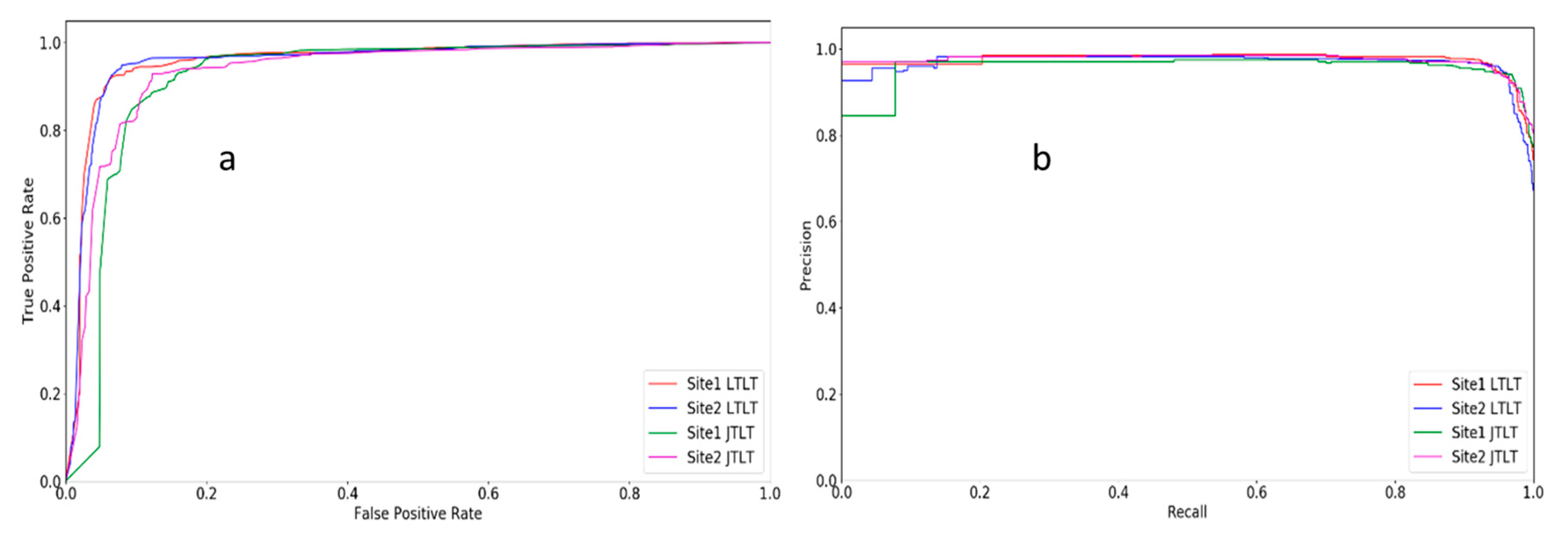
The classifier ability to discriminate classes was evaluated by elaborating receiver operating characteristic (ROC) and precision-recall curves [57,58]. The performance of the classifier was accounted for at the plant-level basis, predicted object versus ground-truthing findings. A random selection of images was implemented in JLTL to account for a balanced training size and comparison between training modes (Figure 4).
The JLTL recall outperforms LTLT in site 1, 0.92 to 0.97. The LTLT better targeted the classification of corn plants (ground-truthing) by reducing “false negatives”, non-corn class (ground-truthing) classified as corn objects. Contrarily, LTLT outperforms JTLT in site 2, recall decreases from 0.95 to 0.93, JTLT presents lower power to correctly classify ground-truth non-corn objects ‘’false negative” as non-corn objects. A higher number of ground-truth corn plants were misclassified as non-corn class objects.
Precision slightly decreases when using JTLT, from 0.97 to 0.94 in site 1. A lower performance of the classifier on the “false positive” detection was documented due to a higher number of ground-truth non-corn objects classified as corn. Precision remained stable (0.96–0.97) in site 2 as an indication that “false positive” detection remained stable across training modes. Nevertheless, the overall accuracy followed a decreasing trend between sites when transitioning from LTLT to JTLT mode as noticed in the area under the curves (AUC) (Figure 5). The LTLT reached an accuracy of 0.96 in both sites and decreased for JTLT to 0.92 for site 1 and 0.93 for site 2. The penalization was mainly due to a lower performance of the JTLT classifier on “false positives” detection, a slightly higher misclassification of ground-truth non-corn objects as corn. Outcomes of the LTLT are in accordance with [17] findings, reporting an accuracy of 0.96, recall of 0.99, and precision of 0.97 between crop and weed objects detection.

3.2. Evaluation Metrics: Spatial Resolution

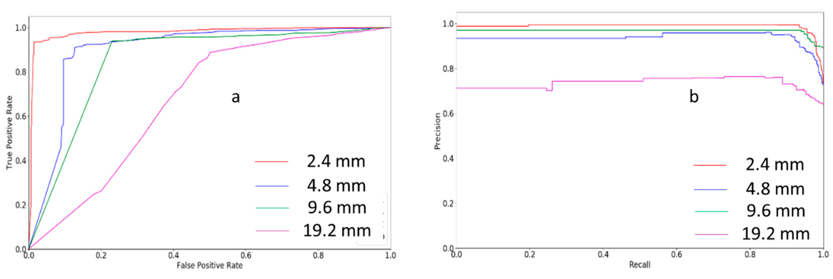
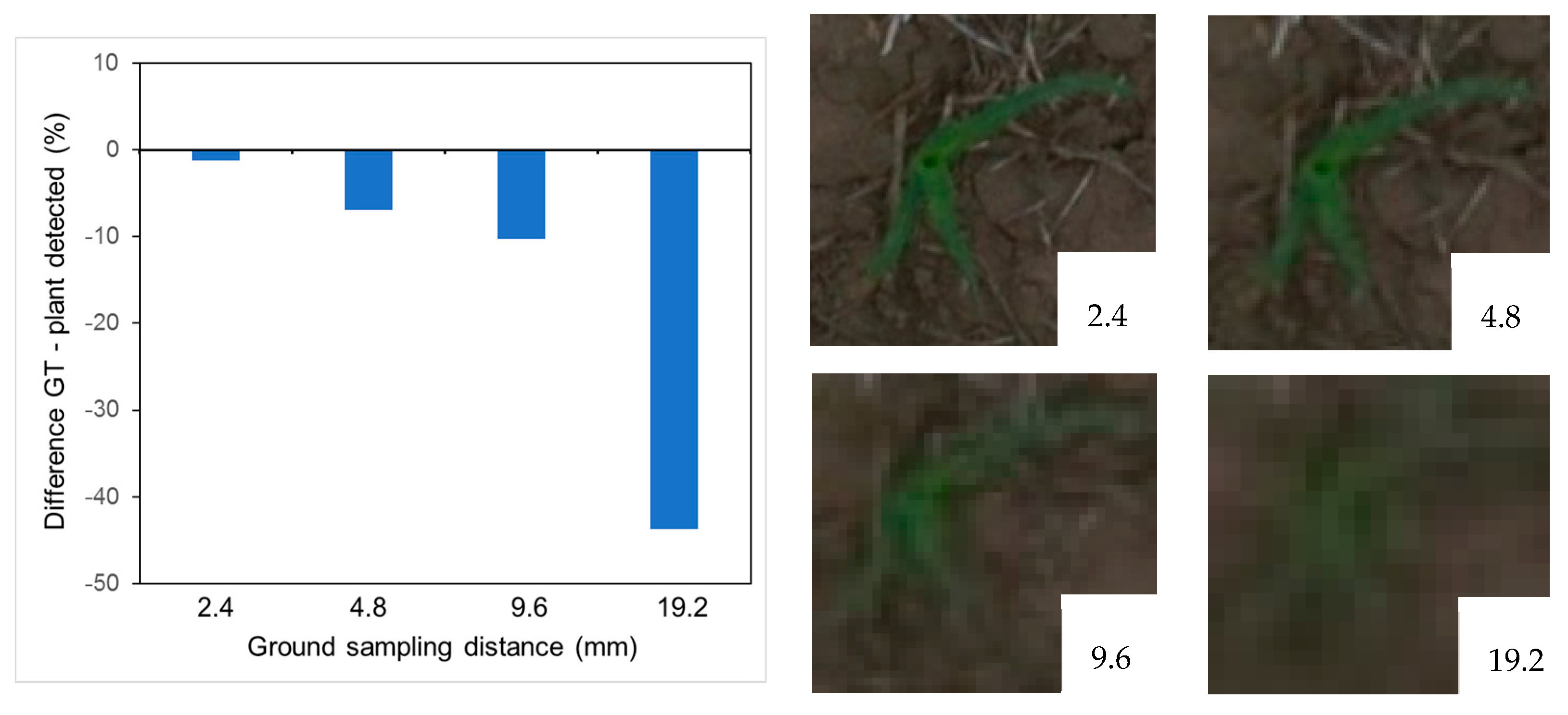
A data downscaled resolution was simulated to evaluate the sensitivity of the workflow on plant detection by recreating degraded resolutions of increasing flight altitudes. The original resolution of 2.4 mm in site 1 was resized to 4.8, 9.6, and 19.2 (Figure 6), simulating 20, 40, and 80 m flight altitudes, respectively. For downscaling the data, simple linear kernels were implemented: 2 × 2, 4 × 4, 8 × 8 mean values of the original pixels scale values into the resulting downscaled pixel. All workflow steps were fully re-implemented at each downscaled resolution. Manual tuning of the pixels row size was utilized to prevent losing and incorrectly accounting for row and inter-row green objects during the training of the downscaled data set.
The classifier accuracy was consistently penalized when the spatial resolution was degraded. Original resolution reached the highest accuracy of 0.96, and decreased to 0.89, 0.85, and 0.68 for each 2.4, 4.8, 9.6, and 19.2 mm resolution, respectively (Figure 6). The P/R curve was penalizing the downscaling following the same trend. Consequently, the overall performance of the classifier was penalized due to a lower sensitivity of geometry as efficient descriptor to differentiate corn and non-corn classes of objects.
It should be noticed that downscaled resolution penalizes the ExG binarization step, and consequently, the ability of the workflow to distinguish objects in the image. The departure between ground-truth objects and the classifier detection assists with a metric on the sensitivity of the workflow to detect green objects in the image. A total of 15 images were selected for this analysis. The departure from ground-truthing (Figure 7) represents the relative distance between the number of true detected objects and the ones reported by the classifier when analyzing the images. When using the original 2.4-mm resolution, the penalization on the sensitivity to detect green objects remains very low (1.5%). When downscaled to 4.8, 9.6, and 19.2 mm, the penalization increases to 6%, 12%, and 42%, respectively.
Downscaled spatial resolution increases the ground sampling distance (GSD), meaning that a larger area on the ground is sensed per pixel unit. Thus, it becomes critical for transitional (green objects borders-background) areas of the image for quality contours delineation in the image. An increasing number of double objects by unit of contour due to “mixed signals” was progressively found when transitioning from finer to downscaled data generating an underestimation of the total number of contours (green objects) (Figure 7).
Current methods propose the use of ground vehicles or satellite data to estimate detailed information of plant status at the fields. The first one evidenced limitations by only being able to cover small areas and depending on good trafficable conditions. The second one does not provide the needed spatial resolution and the performance on this kind of task remains weak. The proposed workflow exploits synergistically the versatility of UAS platforms and a supervised learning procedure to identify crops and non-crops in the field enabling the differentiation between corn plants and weeds early in the season. In addition, the proposed workflow allows the identification and mapping of plants at a very early time in the season using real farm conditions and balancing the classifier performance between both corn and non-corn objects.
A few limitations from the tested method include: (i) late within-growing-season flights are prone to plant overlapping degrading the workflow performance and causing underestimation in the plant count; and (ii) plant density was not evaluated at field-scale since (1) the focus of this project remains in the evaluation of the classifier performance by itself corn plant identification, and (2) accurate field-scale plant density estimation needs accurate and precise ground scaling of the individual imagery via RTK (Real Time Kinematic) or PPK (Post Processed Kinematic) global navigation satellite systems (GNSS). An opportunity for delivering large scale, more efficient, and faster models can be pursued by collecting UAS data using a sub-sampling imagery strategy and spatial analysis. The latter appears as a potential solution for saving computational costs of processing data and preventing a degraded resolution from the original imagery when building an orthomosaic via the stitching procedure.
The main contribution of this paper is related to the development of a procedure to detect corn plants to better guide early season operations for farmers. The foundation of the method relies on the combination of traditional imagery and a supervised learning procedure. The outcome of the workflow allows the digital counting of plants using a low-cost UAS and RGB camera contributing to quantify early-season data of crop performance at on-farm conditions.
Future work should (a) study the potential of spectral and texture descriptors for classes delineation, (b) explore the potential of including multiclass non-corn objects by reducing the internal variance of non-corn objects, and (c) investigate the penalization of high wind conditions in the geometric descriptors and classifier performance.

4. Conclusions

In this work, we implement a workflow to identify corn plants in real field conditions using vegetation detection, feature extraction, and classification using aerial images by exploiting geometric descriptors information. The developed workflow utilizes the spatial arrangement of crops to scale up the training of the classifier. The proposed approach was implemented and tested with imagery data collected via UAS at two farm fields to evaluate the upscaling robustness of the workflow and the potential applications on farm operations. Even though the combined sites’ training (0.92 and 0.93) performed lower than local site training mode (0.96), the combined training mode is still robust for scaling up the processes and, most importantly, to save computational time when dealing with massive amounts of data in the post-processing steps. The original 2.4 mm resolution portrayed the best performance to detect corn objects. Downscaled spatial resolutions gradually negatively impacted the workflow performance at two levels: (i) evidencing a lower sensitivity to detect green contours in the image due to an increased mixed signal (soil background-green objects) that degraded the contours delineation and (ii) decreasing the power of the classifier itself due to a degraded power of the geometry as an effective descriptor to differentiate both classes of objects. Results suggest that the optimal growth for accurate estimation for a field setting of corn plants is between two and three leaves.

Acknowledgments

The authors are thankful for the support from PrecisionHawk and the Kansas Corn Commission. This is contribution 18-309-J from the Kansas Agricultural Experiment Station.

Author Contributions

Sebastian Varela led the design of the workflow and wrote the manuscript; Pruthvidhar Reddy Dhodda led the implementation; William H. Hsu, P. V. Vara Prasad, Yared Assefa, Nahuel R. Peralta, Terry Griffin, Ajay Sharda and Allison Ferguson contributed actively to the revision of the manuscript; Ignacio A. Ciampitti led the design, contributed actively to the discussion and writing of the manuscript.

Conflicts of Interest

The authors declare no conflict of interest.

References

  1. Lauer, J.G.; Rankin, M. Corn Response to Within Row Plant Spacing Variation. Agron. J. 2004, 96, 1464–1468. [Google Scholar] [CrossRef]
  2. Ciampitti, I.A.; Vyn, T.J. A comprehensive study of plant density consequences on nitrogen uptake dynamics of maize plants from vegetative to reproductive stages. Field Crop. Res. 2011, 121, 2–18. [Google Scholar] [CrossRef]
  3. Wiedong, L.; Tollenaar, M.; Stewart, G.; Deen, W. Impact of planter type, planting speed, and tillage on stand uniformity and yield of corn. Agron. J. 2004, 96, 1668–1672. [Google Scholar]
  4. Nielsen, R.L. Stand Establishment Variability in Corn; Publication AGRY-91-01; Purdue University: West Lafayette, IN, USA, 2001. [Google Scholar]
  5. Nafziger, E.D.; Carter, P.R.; Graham, E.E. Response of corn to uneven emergence. Crop Sci. 1991, 31, 811–815. [Google Scholar] [CrossRef]
  6. De Bruin, J.; Pedersen, P. Early Season Scouting; Extension and Outreach. IC-492:7; Iowa State University: Ames, IA, USA, 2004; pp. 33–34. [Google Scholar]
  7. Nielsen, B. Estimating Yield and Dollar Returns from Corn Replanting; Purdue University Cooperative Extension Service: West Lafayette, IN, USA, 2003. [Google Scholar]
  8. Nakarmi, A.D.; Tang, L. Automatic inter-plant spacing sensing at early growth stages using a 3D vision sensor. Comput. Electron. Agric. 2012, 82, 23–31. [Google Scholar] [CrossRef]
  9. Nakarmi, A.D.; Tang, L. Within-row spacing sensing of maize plants using 3D computer vision. Biosyst. Eng. 2014, 125, 54–64. [Google Scholar] [CrossRef]
  10. Shi, Y.; Wang, N.; Taylor, R.K. Automatic corn plant location and spacing measurement using laser line-scan technique. Precis. Agric. 2013, 14, 478–494. [Google Scholar] [CrossRef]
  11. Shrestha, D.S.; Steward, B.L. Size and Shape Analysis of Corn Plant Canopies for Plant Population and Spacing Sensing. Appl. Eng. Agric. 2005, 21, 295–303. [Google Scholar] [CrossRef]
  12. Thorp, K.R.; Steward, B.L.; Kaleita, A.L.; Batchelor, W.D. Using aerial hyperspectral remote sensing imagery to estimate corn plant stand density. Trans. ASABE 2008, 51, 311–320. [Google Scholar] [CrossRef]
  13. Thorp, K.R.; Tian, L.; Yao, H.; Tang, L. Narrow-band and derivative-based vegetation indices for hyperspectral data. Trans. ASAE 2004, 47, 291–299. [Google Scholar] [CrossRef]
  14. Torres-Sanchez, J.; Lopez-Granados, F.; Peña, J.M. An automatic object-based method for optimal thresholding in UAV images: Application for vegetation detection in herbaceous crops. Comput. Electron. Agric. 2015, 114, 43–52. [Google Scholar] [CrossRef]
  15. Salami, E.; Barrado, C.; Pastor, E. UAV flight experiments applied to the remote sensing of vegetated areas. Remote Sens. 2014, 6, 11051–11081. [Google Scholar] [CrossRef] [Green Version]
  16. Peña, J.M.; Torres-Sanchez, J.; Serrano-Perez, A.; de Castro, A.I.; Lopez-Granados, F. Quantifying efficacy and limits of unmanned aerial vehicle UAV technology for weed seedling detection as affected by sensor resolution. Sensors 2015, 15, 5609–5626. [Google Scholar] [CrossRef] [PubMed]
  17. Lottes, P.; Hoferlin, M.; Sander, S.; Muter, M.; Schulze-Lammers, P.; Stachniss, C. An effective classification system for separating sugar beets and weeds for precision farming applications. In Proceedings of the IEEE International Conference on Robotics & Automation (ICRA), Stockholm, Sweden, 16–21 May 2016. [Google Scholar]
  18. López-Granados, F. Weed detection for site-specific weed management: Mapping and real-time approaches. Weed Res. 2011, 51, 1–11. [Google Scholar] [CrossRef]
  19. Torres-Sánchez, J.; Peña, J.M.; de Castro, A.I.; López-Granados, F. Multi-temporal mapping of the vegetation fraction in early-season wheat fields using images from UAV. Comput. Electron. Agric. 2014, 103, 104–113. [Google Scholar] [CrossRef]
  20. Perez-Ortiz, M.; Peña, J.M.; Gutierrez, P.A.; Torres-Sanchez, J.; Hervas-Martınez, C.; Lopez-Granados, F. Selecting patterns and features for between- and within-crop-row weed mapping using UAV imagery. Expert Syst. Appl. 2016, 47, 85–94. [Google Scholar] [CrossRef]
  21. Geipel, J.; Link, J.; Claupein, W. Combined spectral and spatial modeling of corn yield based on aerial images and crop surface models acquired with an unmanned aircraft system. Remote Sens. 2014, 6, 10335–10355. [Google Scholar] [CrossRef]
  22. Zhou, X.; Zheng, H.B.; Xu, X.Q.; He, J.Y.; Ge, X.K.; Yao, X.; Cheng, T.; Zhu, Y.; Cao, W.X.; Tian, Y.C. Predicting grain yield in rice using multi-temporal vegetation indices from UAV-based multispectral and digital imagery. ISPRS J. Photogramm. Remote Sens. 2017, 130, 246–255. [Google Scholar] [CrossRef]
  23. Bendig, J.; Willkomm, M.; Tilly, N.; Gnyp, M.L.; Bennertz, S.; Qiang, C.; Miao, Y.; Lenz-Wiedemann, V.I.S.; Bareth, G. Very high resolution crop surface models (CSMs) from UAV-based stereo images for rice growth monitoring in Northeast China. Int. Arch. Photogramm. Remote Sens. Spat. Inf. Sci. 2013, 40, 45–50. [Google Scholar]
  24. Mathews, A.J.; Jensen, J.L.R. Visualizing and Quantifying Vineyard Canopy LAI Using an Unmanned Aerial Vehicle (UAV) Collected High Density Structure from Motion Point Cloud. Remote Sens. 2013, 5, 2164–2183. [Google Scholar] [CrossRef]
  25. Yao, X.; Wang, N.; Liu, Y.; Cheng, T.; Tian, Y.; Chen, Q.; Zhu, Y. Estimation of Wheat LAI at Middle to High Levels Using Unmanned Aerial Vehicle Narrowband Multispectral Imagery. Remote Sens. 2017, 9, 1304. [Google Scholar] [CrossRef]
  26. Haboudane, D.; Miller, J.R.; Pattey, E.; Zarco-Tejada, P.J.; Strachan, I.B. Hyperspectral vegetation índices and novel algorithms for predicting green LAI of crop canopies: Modeling and validation in the context of precision agriculture. Remote Sens. Environ. 2004, 90, 337–352. [Google Scholar] [CrossRef]
  27. Pölönen, I.; Saari, H.; Kaivosoja, J.; Honkavaara, E.; Pesonen, L. Hyperspectral imaging based biomass and nitrogen content estimations from light-weight UAV. In Proceedings of the SPIE Remote Sensing, Dresden, Germany, 23–26 September 2013. [Google Scholar]
  28. Potgieter, A.B.; George-Jaeggli, B.; Chapman, S.C.; Laws, K.; Suárez Cadavid, L.A.; Wixted, J.; Wason, J.; Eldridge, M.; Jordan, D.R.; Hammer, G.L. Multi-spectral imaging from an unmanned aerial vehicle enables the assessment of seasonal leaf area dynamics of sorghum breeding lines. Front. Plant Sci. 2017, 8. [Google Scholar] [CrossRef] [PubMed]
  29. De Souza, C.H.W.; Lamparelli, R.A.C.; Rocha, J.V.; Magalhaes, P.S.G. Height estimation of sugarcane using an unmanned aerial system (UAS) based on structure from motion (SfM) point clouds. Int. J. Remote Sens. 2017, 38, 2218–2230. [Google Scholar] [CrossRef]
  30. Iqbal, F.; Lucieer, A.; Barry, K.; Wells, R. Poppy Crop Height and Capsule Volume Estimation from a Single UAS Flight. Remote Sens. 2017, 9, 647. [Google Scholar] [CrossRef]
  31. Caturegli, L.; Corniglia, M.; Gaetani, M.; Grossi, N.; Magni, S.; Migliazzi, M.; Angelini, L.; Mazzoncini, M.; Silvestri, N.; Fontanelli, M.; et al. Unmanned Aerial Vehicle to Estimate Nitrogen Status of Turfgrasses. PLoS ONE 2016, 11, e0158268. [Google Scholar] [CrossRef] [PubMed]
  32. Clevers, J.G.P.W.; Kooistra, L. Using Hyperspectral Remote Sensing Data for Retrieving Canopy Chlorophyll and Nitrogen Content. IEEE J. Sel. Top. Appl. Earth Obs. Remote Sens. 2012, 5, 574–583. [Google Scholar] [CrossRef]
  33. Uto, K.; Seki, H.; Saito, G.; Kosugi, Y. Characterization of Rice Paddies by a UAV-Mounted Miniature Hyperspectral Sensor System. IEEE J. Sel. Top. Appl. Earth Obs. Remote Sens. 2013, 6, 851–860. [Google Scholar] [CrossRef]
  34. Gomez-Candon, D.; Virlet, N.; Labbe, S.; Jolivot, A.; Regnard, J.L. Field phenotyping of water stress at tree scale by UAV-sensed imagery: New insights for thermal acquisition and calibration. Precis. Agric. 2016, 17, 786–800. [Google Scholar] [CrossRef]
  35. Gonzalez-Dugo, V.; Zarco-Tejada, P.; Nicolas, E.; Nortes, P.A.; Alarcon, J.J.; Intrigliolo, D.S.; Fereres, E. Using high resolution UAV thermal imagery to assess the variability in the water status of five fruit tree species within a commercial orchard. Precis. Agric. 2013, 14, 660–678. [Google Scholar] [CrossRef]
  36. Berni, J.; Zarco-Tejada, P.; Suarez, L.; Fereres, E. Thermal and narrowband multispectral remote sensing for vegetation monitoring from an unmanned aerial vehicle. IEEE Trans. Geosci. Remote Sens. 2009, 47, 722–738. [Google Scholar] [CrossRef] [Green Version]
  37. Jin, X.; Liu, S.; Baret, F.; Hemerlé, M.; Comar, A. Estimates of plant density of wheat crops at emergence from very low altitude UAV imagery. Remote Sens. Environ. 2017, 198, 105–114. [Google Scholar] [CrossRef]
  38. Guo, W.; Rage, U.K.; Ninomiya, S. Illumination invariant segmentation of vegetation for time series wheat images based on decision tree model. Comput. Electron. Agric. 2013, 96, 58–66. [Google Scholar] [CrossRef]
  39. Montalvo, M.; Pajares, G.; Guerrero, J.M.; Romeo, J.; Guijarro, M.; Ribeiro, A.; Ruz, J.J.; Cruz, J.M. Automatic detection of crop rows in maize fields with high weeds pressure. Expert Syst. Appl. 2012, 39, 11889–11897. [Google Scholar] [CrossRef] [Green Version]
  40. Gnädinger, F.; Schmidhalter, U. Digital counts of maize plants by unmanned aerial vehicles (UAVs). Remote Sens. 2017, 9, 544. [Google Scholar] [CrossRef]
  41. Baxes, G.A. Digital Image Processing, Principles and Application; John Wiley & Sons: Hoboken, NJ, USA, 1994; ISBN 0-471-00949-0. [Google Scholar]
  42. Savitzky, A.; Golay, M.J.E. Smoothing and differentiation of data by simplified least squares procedures. Anal. Chem. 1964, 36, 1627–1639. [Google Scholar] [CrossRef]
  43. Tokekar, P.; Hook, J.V.; Mulla, D.; Isler, V. Sensor planning for a symbiotic UAV and UGV system for precision agriculture. IEEE Trans. Robot. 2016, 32, 5321–5326. [Google Scholar] [CrossRef]
  44. Hale Group. The Digital Transformation of Row Crop Agriculture, AgState Electronic Survey Findings. 2014. Available online: http://www.iowacorn.org/document/filelibrary/membership/agstate.AgState_Executive_Summary_0a58d2a59dbd3.pdf (accessed on 19 December 2017).
  45. Henry, M. Big Data and the Future of Farming; Australian Farm Institute Newsletter: Surry Hills, Australia, 2015; Volume 4. [Google Scholar]
  46. Meier, L.; Honegger, D.; Pollefeys, M. PX4: A node-based multithreaded open source robotics framework for deeply embedded platforms. In Proceedings of the IEEE International Conference on Robotics & Automation (ICRA), Seattle, WA, USA, 26–30 May 2015. [Google Scholar]
  47. Laganiere, R. OpenCV 2 Computer Vision Application Programming Cookbook; Packt Publishing Ltd.: Birmingham, UK, 2014. [Google Scholar]
  48. Pedregosa, F.; Varoquaux, G.; Gramfort, A.; Michel, V. Scikit-learn: Machine Learning in Python. J. Mach. Learn. Res. 2011, 12, 2825–2830. [Google Scholar]
  49. Meyer, G.E.; Neto, J.C. Verification of color vegetation indices for automated crop imaging applications. Comput. Electron. Agric. 2008, 63, 282–293. [Google Scholar] [CrossRef]
  50. Otsu, N. A threshold selection method from gray-level histogram. IEEE Trans. Syst. Man Cybern. 1979, 9, 62–66. [Google Scholar] [CrossRef]
  51. Hough, P.V.C. A Method and Means for Recognizing Complex Patterns. U.S. Patent 3,069,654, 18 December 1962. [Google Scholar]
  52. Guyon, I.; Elisseeff, A. An Introduction to Variable and Feature Selection. J. Mach. Learn. Res. 2003, 3, 1157–1182. [Google Scholar]
  53. Alaydin, E. Introduction to Machine Learning; MIT Press: Cambridge, MA, USA, 2004. [Google Scholar]
  54. Patel, N.; Upadhyay, S. Study of various decision tree pruning methods with their empirical comparison in WEKA. Int. J. Comput. Appl. 2012, 60, 20–25. [Google Scholar] [CrossRef]
  55. Breiman, L.; Friedman, J.; Olshen, R.; Stone, C. Classification and Regression Trees; Wadsworth: Belmont, CA, USA, 1984. [Google Scholar]
  56. Eastwood, M.; Gabrys, B. Generalised bottom-up pruning: A model level combination of decision trees. Expert Syst. Appl. 2012, 39, 9150–9158. [Google Scholar] [CrossRef]
  57. Powers, D.M.W. Evaluation: From precision, recall and F-measure to ROC, informedness, markedness and correlation. J. Mach. Learn. Technol. 2011, 2, 37–63. [Google Scholar]
  58. Fawcett, T. An introduction to ROC analysis. Pattern Recognit. Lett. 2006, 27, 861–874. [Google Scholar] [CrossRef]
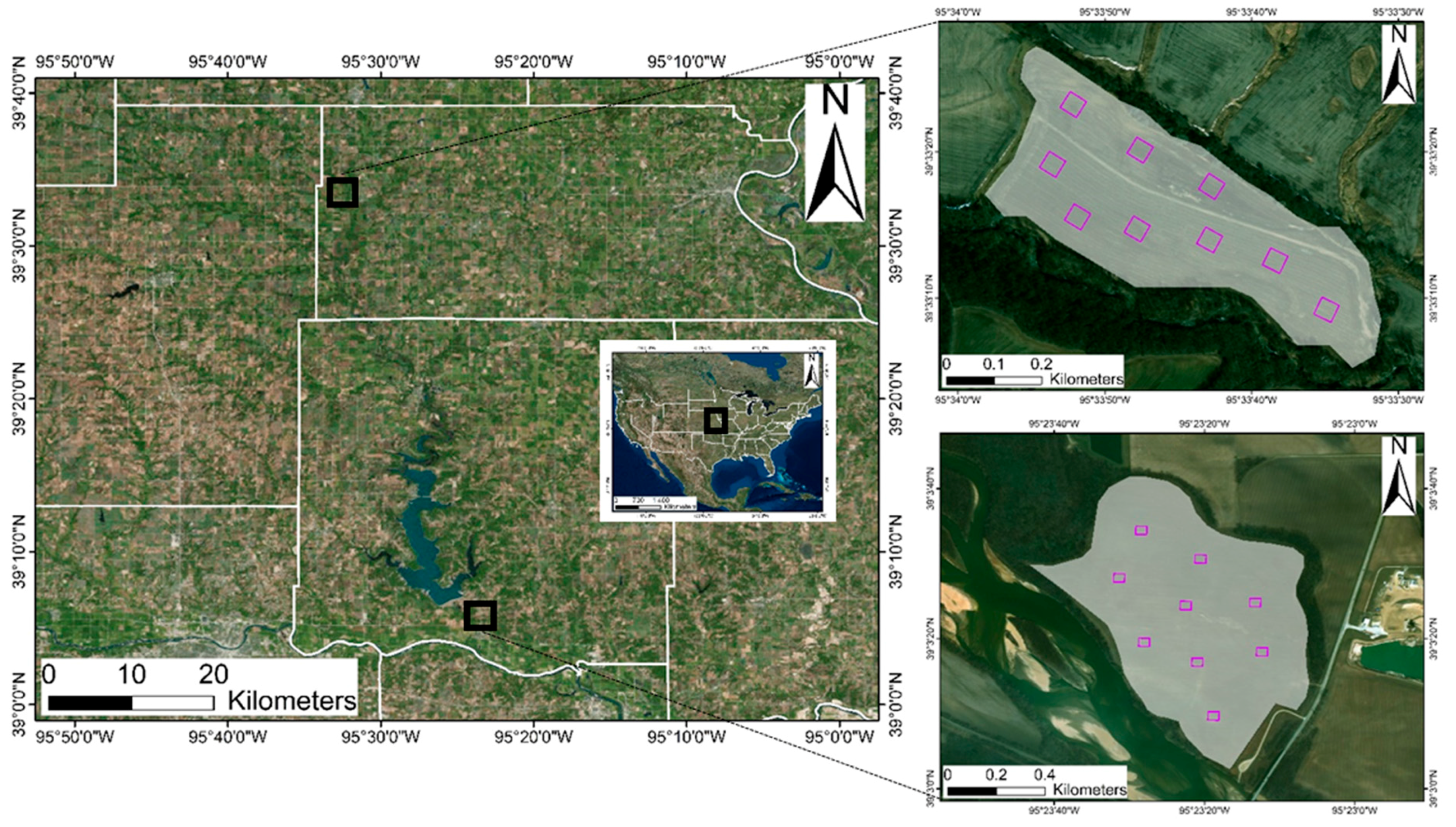
Figure 1. Left: On-farm fields located in the northeast region of Kansas. Top-right: Site 1, Atchison, KS; bottom-right: Site 2, Jefferson, KS. Purple squares = field sampled areas.
Remotesensing 10 00343 g001
Figure 2. Workflow for plant estimation via unmanned aerial systems (UAS). (A) data pre-processing, (B) training, (C) cross-validation, and (D) testing.
Remotesensing 10 00343 g002
Figure 3. Diagram of the Excess Greenness (ExG) index projection, local-maxima smoothing, and thresholding for rows location.
Remotesensing 10 00343 g003
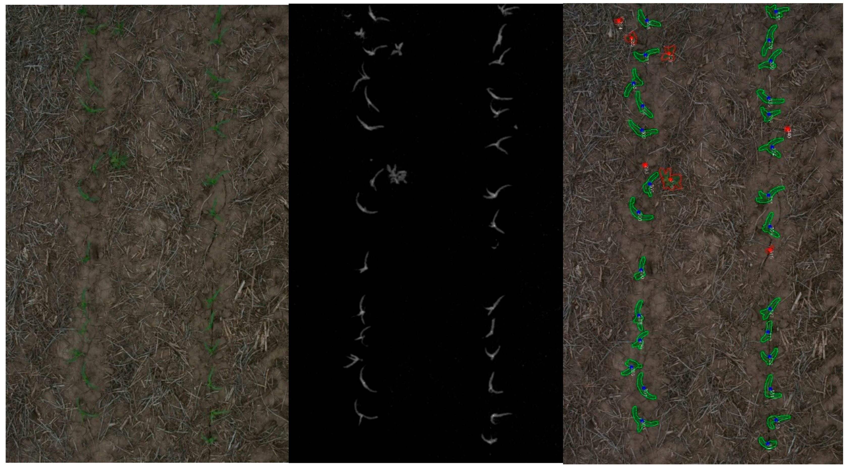
Figure 4. Left: RGB, center: ExG, right: classifier output on testing data in site 1, green contours: corn objects, red contours: non-corn objects.
Remotesensing 10 00343 g004
Figure 5. Receiver operating characteristic (ROC) curves (a) and positive rate (PR) plots (b) based on testing data for each site.
Remotesensing 10 00343 g005
Figure 6. ROC curves (a), and PR plots (b) of downscaled testing data set in testing resolutions.
Remotesensing 10 00343 g006
Figure 7. Difference between ground-truth and objects detected by the classifier as a function of spatial resolution.
Remotesensing 10 00343 g007
Table 1. Information about sites and flights during the 2017 growing season.
FieldsPrevious CropPlanting Date (DOY)Growth StageFlight Day (DOY)Flight Altitude (m)
Site 1Soybean116v213510
Site 2Soybean130v2–v315310
Table 2. Data sets used for training and testing of the classifier.
Site 1Site 2
Data SetTrainingTestingTrainingTesting
Images94758775
Contours17,60815,37816,85515,246