Abstract
The thickness of oil spills on the sea is an important but poorly studied topic. Means to measure slick thickness are reviewed. More than 30 concepts are summarized. Many of these are judged not to be viable for a variety of scientific reasons. Two means are currently available to remotely measure oil thickness, namely, passive microwave radiometry and time of acoustic travel. Microwave radiometry is commercially developed at this time. Visual means to ascertain oil thickness are restricted by physics to thicknesses smaller than those of rainbow sheens, which rarely occur on large spills, and thin sheen. One can observe that some slicks are not sheen and are probably thicker. These three thickness regimes are not useful to oil spill countermeasures, as most of the oil is contained in the thick portion of a slick, the thickness of which is unknown and ranges over several orders of magnitude. There is a continuing need to measure the thickness of oil spills. This need continues to increase with time, and further research effort is needed. Several viable concepts have been developed but require further work and verification. One of the difficulties is that ground truthing and verification methods are generally not available for most thickness measurement methods.
1. Introduction
There is a need to measure oil slick thickness [1]. There are presently few reliable methods, either in the laboratory or in the field, for accurately measuring oil-on-water slick thickness [1]. In addition to measuring slick thickness, there is little information published on the thickness regimes of oil spills. The knowledge of slick thickness would certainly have many uses in the oil spill field, which include:
- Determining the size of a leak or discharge
- Legal action for discharges
- Determination of the effectiveness of oil spill countermeasures—particularly in situ burning and chemical dispersion
- Assessing the fate of the oil
- Understanding the physics of oil spill spreading
- Studying the physics of oil evaporation
- Optimizing oil spill countermeasures
- Understanding the physical distribution of oil on the sea and the rates of spreading.
Slick thickness measurements are now at an early stage of development. There are many proposed solutions. The few solutions that are available are complex and involve extensive equipment. There are no simple solutions.
There are numerous problems in the field. First and foremost, there are few available field measurement techniques, only passive microwave. Thus, we know little about how slicks are distributed and what the ranges of thickness might be. Further, we do not really understand how this relates to oil type, water content, sea conditions, etc. Water-in-oil emulsions form and have quite different appearances and properties with respect to non-emulsified slicks. The existing slick thickness measurement methods may not work on emulsions.
An important question is the determination of the relevant thickness ranges. Figure 1 illustrates the orders of magnitude relevant to an oil spill situation. An important point is that the easily determined visual ranges are orders of magnitude below the relevant thickness ranges needed for oil spill countermeasures to work. This figure also illustrates the errors that would occur if one used incorrect information on thickness to determine the volume. The errors could be as large as orders of magnitude.
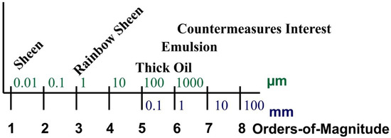
Figure 1.
Illustration of the relevant oil spill thickness regimes.
2. The Properties of Oil Affecting Thickness Determination
Crude oils are mixtures of hydrocarbon compounds ranging from smaller, volatile compounds to very large, non-volatile compounds [2]. This mixture of compounds varies according to the geological formation of the area in which the oil is found and strongly influences the properties of the oil. For example, crude oils that consist primarily of large compounds are viscous and dense. Petroleum products such as gasoline or diesel fuel are mixtures of fewer compounds, and thus their properties are more specific and less variable. Oils also contain varying amounts of other elements and metals. These minor ingredients, for the most part, do not play a role in oil spill detection or measurement. The hydrocarbons found in oils can be characterized by their structure. The hydrocarbon structures found in oil are saturates, aromatics, and polar compounds. The saturate group of components in oils consists primarily of alkanes, which are compounds of hydrogen and carbon with the maximum number of hydrogen atoms around each carbon. Thus, the term ‘saturate’ is used because the carbons are ‘saturated’ with hydrogen. Larger saturate compounds are often referred to as ‘waxes’. Saturate compounds have a modest chemical signature by themselves and thus do not play a strong role in oil spill remote sensing.
The aromatic compounds include at least one benzene ring of six carbons. These types of aromatic compounds may have a spectral signature, which, however, is highly variable with respect to the chemical composition. This spectral signature also changes over time after a spill, as the lighter components evaporate. Polar compounds are those that have a significant molecular charge as a result of bonding with compounds such as sulfur, nitrogen, or oxygen. These compounds are rather inert and do not have a significant spectral signature.
In terms of color, there is little differentiation between oils, especially for crude oils which are generally brown to black. There are small spectral differences in the visible region of the spectrum [3]. This changes little as the oil evaporates or weathers after a spill.
Water-in-oil emulsions sometimes form after oil products are spilled. These emulsions, often called “chocolate mousse” or “mousse” by oil spill workers, make the cleanup of oil spills very difficult [4]. When water-in-oil emulsions form, the oil physical properties of the oil change dramatically. As an example, stable emulsions contain from 60 to 80% of water, thus expanding the spilled material by 2 to 5 times its original volume. Most importantly, the viscosity of the oil typically changes from a few hundred mPa.s to about 100,000 mPa.s, which corresponds to an increase by a factor of 500 to 1000. A liquid product is changed into a heavy, semisolid material. Importantly, four water-in-oil types have been identified: stable emulsions are reddish-brown semisolid substances with an average water content of about 70–80% on the day of formation, which remains about the same one week later [4]. Meso-stable water-in-oil emulsions are reddish-brown viscous liquids with an average water content of 60–65% on the first day of formation and of less than 30% one week later. Entrained water-in-oil types are black viscous liquids with an average water content of 40–50% on the first day of formation and of less than 28% one week later. Many oils do not uptake water to a significant degree and remain unchanged in this respect. Importantly, the dielectric properties of the resulting products are very much changed. Oil has a dielectric constant of about 2, and water of about 80. The water-in-oil types would have varying dielectric constants, varying between these two extremes. This strongly affects the remote sensing properties such as microwave reflection.
3. Proven Techniques
3.1. Microwave Reflectivity
Oil on the sea acts as a matching dielectric layer to the incoming natural microwave radiation (30 to 300 GHz) [5]. The natural microwave radiation encountering this oil layer causes its surface brightness to increase as a function of the oil layer thickness, as the emissivity of the oil layer (0.8) is greater than that of water (0.4) [5]. The microwave brightness of the slick varies with thickness, however, in a cyclical fashion as shown in Figure 2. This means that a particular microwave brightness may imply one of several thicknesses [6,7]. One method to overcome this is to use multiple frequencies as shown in Figure 3. This will reduce the ambiguity to a certain extent. One should note, however, that the microwave brightness is also influenced by a number of other factors, such as the weather and sea conditions and the type of oil. Another important factor one should note is that, in practice, the microwave response requires calibration to determine the response factors. This is typically carried out using plastic sheets of the appropriate size. Plastic has about the same dielectric constant as oil.
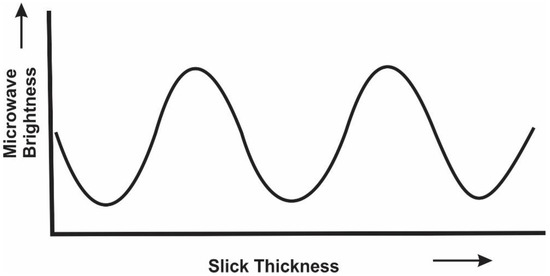
Figure 2.
The cyclic relationship between microwave brightness and oil thickness.
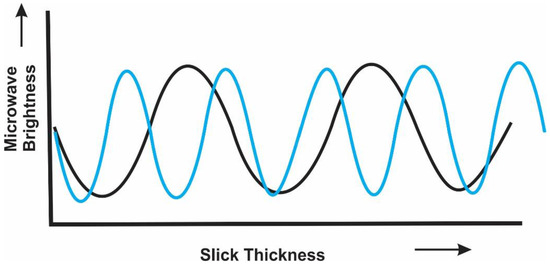
Figure 3.
Use of a dual- or higher-frequency microwave system can eliminate some of the uncertainty related to thickness.
Hollinger and Mennella studied a series of small test slicks off the coast of New Jersey [6]. Using a two-frequency microwave receiver, they plotted the slick thickness of the slicks. These experiments formed the basis for much of later work, as these particular test slicks had the profile of a fried egg, that is, there was a thick center portion and a large area of thin slick around this thick portion. This geometry may, in fact, largely be applicable to a small test slick, as spreading would not be complete as in an instantaneous or continuous slick that has been on the water for a day or so.
Skou and coworkers reviewed microwave sensing extensively and carried out laboratory and at-sea experiments to measure oil thicknesses using a three-frequency radiometer (5, 17, and 34 GHz) [8,9]. It was shown that an accurate thickness profile could be drawn given certain major compensations. First, the 5 GHz signal gave much greater thicknesses than the 34 GHz channel, and this had to be compensated for. Second, after a certain thickness, the sensor readings generally become ambiguous, in this case it was 0.5 mm. Thirdly, as the spatial resolution is low, averaging takes place, and this usually results in an overestimation of the oil amount. A theoretical study of the applicability of microwave to water-in-oil emulsions shows that these might not be detected. The images of an experimental 40 m3 spill are shown in Figure 4.
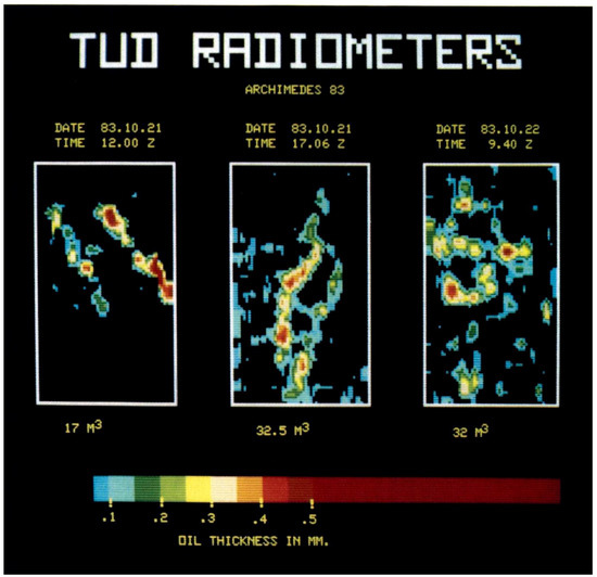
Figure 4.
An image of a slick characterized by an early microwave sensor by Skou et al. [8,9]. The integrated slick volumes are written under each figure. These images were taken using a 3-band passive microwave imager operating at 5, 17, and 34 GHz. This particular system is applicable to about 0.5 mm, after which the signal is ambiguous. Thus, this particular system would not be useful for thicker and freshly spilled oils. Therefore, it is noted that the first scan on the test slick underestimated the amount of 17 m3 versus about 40 m3 spilled. The scans, later on the first day and on the second day, had approximately the right amounts of oil. Because of low spatial resolution, the averaging of the surface takes place, resulting in higher estimates of oil. This is shown by the 32.5 and 32 m3 amounts on the last part of the first day and on the second day of flights. Presumably, these amounts should have been slightly lower because of slick evaporation. It is also important to note that the sheens are not seen in microwave images. This early microwave system did not have high resolution in addition to not being well calibrated.
Pelyushenko developed a method to calculate oil slick thickness using microwaves [10]. The difference in incoming versus reflected radiation from an oil slick was measured using a pair of orthogonal receivers. The vertical and horizontal polarization temperatures after measurement were calculated as differentials from unoiled water. The thickness then was calculated by the typical methods. Cyclic redundancy was again overcome by using a 2-frequency receiver (11.5 and 34 GHz). To measure the polarizations and the orthogonal waves, 32 horns were used in the 34 GHz system and 12 horns in the 11.5 GHz system. Laboratory and tank tests were carried out; however, the success of the full-scale version is unknown.
The only instrument currently available for measuring slick thickness is the Optimare three-channel microwave instrument [11]. This instrument is claimed to have a capability of measuring from 0.05 to 3 mm. Versions of this instrument have been sold for about 10 years. There are not much public data available, as most of the obtained measurements have been used for legal prosecution purposes. Figure 5 shows a slick imaged using the Optimare instrument.
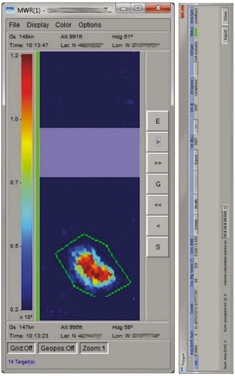
Figure 5.
An image of a slick characterized by microwave (Photo from Nils Robbe, Optimare, 2017). The colors of the image represent the thicknesses, and the scale is on the left-hand side of the image (ranges from 0.2 to 1.2 mm in this case). This is an image from the usual aircraft display, and several pieces of information are normally available, including location and area of the slick (here this is 0.008 km2, yielding a volume of 1897 L). The data were measured using a 3-band passive microwave imager operating at 18, 36, and 89 GHz. This instrument is commercially available.
Hammoud et al. studied oil spill detection as a possibility from a drone platform [12]. In examining the possibilities, they calculated the reflectivities of the microwave signals (i.e., radar) from slicks of various thicknesses. It was noted that the simple reflectivities showed cyclical behaviors at the various frequencies chosen for the calculation (4.5 GHz, 8 GHz and 11 GHz). This dielectric reflection calculation showed that if one used the frequencies mentioned, that detection of oil could be confirmed, and the thickness would also be measured. This paper shows that the standard microwave reflectivity could be used as a slick thickness testing device. The concept of Hammoud et al. of using three radar frequencies might be less viable as a drone method because of the large weight and cost.
Microwave radiometry is a proven technique for remotely measuring the thickness of fresh oil on the water surface. Limitations include the question of how weathering and water uptake affect this ability. Water uptake is expected to at least degrade the signal, if not to remove it entirely.
3.2. Sonic Travel Time
The speed of sound is relatively constant in various liquid oils. Therefore, measuring the time of travel from the top surface to the water–oil interface can provide a measure of oil thickness. This might be done remotely using laser acoustics [13,14,15]. The Laser Ultrasonic Remote Sensing of Oil Thickness (LURSOT) sensor consists of three lasers, one of which is coupled to an interferometer to accurately measure oil thickness [16,17,18,19,20,21]. The sensing process is initiated with a thermal pulse created in the oil layer by the absorption of a powerful CO2 laser pulse. A rapid thermal expansion of the oil occurs near the surface where the laser beam was absorbed, which causes an acoustic pulse of high frequency and large bandwidth (~15 MHz for oil). The acoustic pulse travels down through the oil until it reaches the oil–water interface where it is partially transmitted and partially reflected back towards the oil–air interface, where it slightly displaces the oil’s surface. The time required for the acoustic pulse to travel through the oil and back to the surface again is a function of the thickness and of the acoustic velocity of the oil. The displacement of the surface is measured by a second laser probe beam aimed at the surface. The motion of the surface induces a phase or frequency shift (Doppler shift) in the reflected probe beam. This phase or frequency modulation of the probe beam can then be demodulated with an interferometer. The thickness can be determined from the time of propagation of the acoustic wave between the upper and lower surfaces of the oil slick. Laboratory tests have confirmed the viability of the method, and a test unit has been flown to confirm its operability. Figure 6 shows the first airborne measurement of slick thickness. This particular slick was about 6 mm thick. The slick thickness limit depends on the rise time of the YAG laser measuring the acoustic pulse. The measuring ability of the prototype system is thought to be from about 2 to 15 mm. This might be convenient, since the limits of the other proven remote sensing technique, passive radiometry, are from about 0.5 to about 3 mm. Therefore, both systems might be needed to measure thin and thick slicks.
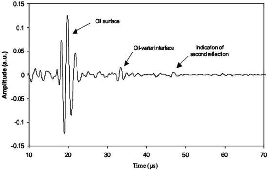
Figure 6.
The signal from a 3-laser thickness sensor. The time of the first return pulse corresponds to a thickness of about 6 mm. This was measured by a prototype sensor mounted in an aircraft and flying over containers with various thicknesses of oil on water.
Li et al. studied oil thickness using sonic travel time between the oil surface and the oil–water interface [22]. They used a 355 nm pulsed laser to generate ultrasonic waves on the oil surface and a scanning laser Doppler vibrometer to detect the surface motion. The laser Doppler vibrometer measures the amplitude and frequency of the acoustic signals on the surface of the oil and thus both the input and the return acoustic signals. The time of travel was used to measure oil thickness.
The measurement of sonic travel time through a slick offers a means to measure the oil slick thickness. The effects of oil weathering on an acoustic thickness measuring system are unknown, as the speed of sound in an emulsion or water-containing oil is unknown. Further, such a system would be best to scan, as the thickness of a small oil spot may not be entirely useful or would be difficult to extrapolate to a larger area.
3.3. Visual Thickness Estimation of Thin Slicks
In the past, a very important tool for working with oil spills was thought to be the relationship between appearance and thickness. Very little quantitative research work has been done on this topic in recent times because thickness charts have been available for many years. In fact, the present thickness charts actually date from 1930 [23]. It had already been recognized before this time that thin slicks on water had consistent or nearly consistent appearances. A series of experiments were conducted at that time and resulted in charts that are still used. Only a few experiments have been done in recent years, most of which confirmed the thickness–appearance relationships [24].
The acceptance of this early work without further question might be reconsidered, especially in view of the fact that several factors were probably not addressed:
- Effect of slick heterogeneity—Oils, especially heavier ones, do not form a consistent flat slick on the water surface. Even visual examination shows a type of ‘fried egg’ or similar profile. Most past experiments presumed that the slick was homogeneously thick. Furthermore, many slicks do not cover homogeneously an entire area. The effect of surface tension is to pull some oils together so that multiple little slicks may be formed rather than one uniform slick.
- Effect of evaporation—The early slick appearance experiments ignored the effect of evaporation in calculations of thickness, nor was it recognized that evaporation was an exponential or logarithmic phenomenon. Sometimes, experimenters presumed that the amount of oil put on the surface was still present hours afterwards. The effect of evaporation is to lower the amount of oil having the stated appearance.
- Effect of the view angle—It is known that the view angle is critical to observing slicks on water, especially with respect to the sun. How this affects thresholds was not fully explored. Some experiments did include the viewing angle and found that the slick’s appearance changed significantly.
- Effect of waves on the surface—The appearance of oil slicks on calm water versus that with different wave conditions could be different. Perhaps, it is only a matter of contrast or differing discrimination.
- Effect of atmospheric and viewing conditions—Another factor that might be important is the presence of haze and of cloud cover. Haze strongly reduces visibility. It has been observed that slicks are often less visible in the absence of a cloud cover. Glitter from the sea is known to cause viewing problems.
- Effect of oil type—It is known that dark oils are more visible on the surface than gasoline or diesel fuel. It is not known if this effect is also true after the very onset of visibility.
The appearance factors are very important because they provide the only current means for estimating the amount of oil in thin sheens on the sea. There are no means for estimating the amounts of oil in thick slicks on the sea. It is very important to note that most spilled oil is in the thick slicks, whose thicknesses cannot be estimated visually. The slick appearance factors are used by cleanup personnel to direct cleanup operations, by surveillance personnel who patrol for illicit discharges, and by scientists to predict the fate and behaviour of an oil.
Hornstein reviewed the theoretical approaches and used interference phenomena to correlate the threshold of rainbow colours to slick thickness [25,26]. The appearance of the rainbow colours is the result of constructive and destructive interference of the light waves reflected from the air–oil interface with those reflected from the oil–water interface. The difference in optical path lengths for these two types of waves depends on the refractive index of the oil. The refractive index of a given wavelength results in a difference in the optical path length. This difference can be given as:
where: ΔL is the difference in optical path length; t is the film thickness; μ is the refractive index of the film; I is the angle of light incidence.
ΔL = 2t (μ2 − sin2I)½
Hornstein points out that if ΔL contains a whole number of wavelengths, then the maximum destructive interference will occur. If ΔL contains an odd number of half wavelengths, then the maximum constructive interference will occur.
Then, the maximum destructive interferences occur at:
where λ is the wavelength under consideration, and x is a whole number as 1,2,3,4 etc.
λ = ΔL/x
The maximum constructive interferences occur at:
where x is a whole odd number as 1,3,5,7 etc.
λ = 2ΔL/x
Tables of constructive and destructive wavelengths can be written [25,26]. These then result in a colour chart for visible oil, with descriptions such as the following: thickness less than 0.15 μm—no colour apparent, thickness of 0.15 μm—warm tone apparent, thickness of 0.2 to 0.9 μm—variety of colours (e.g., rainbow), thickness greater than 0.9 μm—colours of less purity. This corresponds to the observed onset noted in the experiments. Figure 7 shows a rainbow sheen, the only spill thickness that shows a distinctive visual signature.
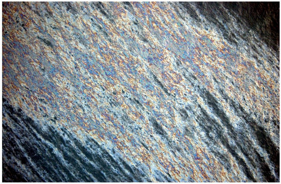
Figure 7.
A fresh discharge from a vessel which has a rainbow color appearance.
Hornstein also calculated the differential reflectivity of oil and water [25,26]. He calculated that, at an incidence angle of 30°, the reflectivity of oil is 0.041, and that of water is 0.021. At 60°, oil shows a reflectivity of 0.09 and water of 0.06, and at 75°, oil has a reflectivity of 0.25 and water of 0.21. These angles are calculated as the angle of light incidence from the normal, and thus show that reflectivity increases as the angle of viewing becomes less vertical. The reflectivity may explain the visibility of very thin films of oil (less than shown by coloration) on the water surface. This calculation demonstrates that the viewing angle is important and that the greatest contrast is seen from near vertical angles.
Many different codes were developed, largely based on older work, and some with newer experimental work, some of which are listed in Table 1 [24]. The findings to date include the following:

Table 1.
Relationships between Appearance and Slick Thickness.
- The utility of thicknesses derived from oil color codes is very limited. The only reliable color codes are those corresponding to very thin oil slicks. Most of the oil is located in the thick portions of the slick. For larger spills the appearance codes are not useful.
- The only reliable thickness indications are the thin sheen and the rainbow portions. The rainbow portion is the only unique thickness range at about 0.2 to about 1 to 3 µm at the top end.
- There are many influences on the appearance, including the sun angle with respect to the viewer, the view angle, the oil type the sea conditions, the water coloration, the presence of debris, etc.
- There is no supporting evidence for any colorations or relationships for the thicker portions of the slick.
- There are only three thicknesses that can be identified: sheen, rainbow slicks, and thicker oil. A fourth group, emulsions, might be useful, but their thickness varies and is not well understood. Again, it should be noted that this classification is not useful for most spills.
One of the color codes that emerged in recent years is that of the Bonn Agreement [27]. This is shown in Table 2. It is different from any other code with respect to the thicker parts. The basis for these thicker appearances is apparently derived from some experimental work that, however, was never reviewed or published. This is interesting in that the same group issued a report supporting the conventional codes and decrying any efforts to codify thicker slicks [28]. A second issue is the calling of the thicker portion ‘metallic’, which, again, is a departure from convention. Most observers agree that there may not be a commonly accepted color described as metallic. Several parties have questioned this code [29,30,31,32]. There have been no scientific papers supporting this thicker code. There is strong evidence that the clearest signal for thickness is only with the rainbow sheen, as shown in Figure 7. The current ASTM standard considers the conventional thin appearance codes and is shown in Table 3 [33].
Table 2.
The Bonn Agreement Code.
Table 3.
ASTM Relationship of Thickness to Appearance.
4. Concepts for Estimating Slick Thickness
4.1. Near-Infrared Reflectance
Several workers have proposed to use reflection or specular reflection from slicks in the near-infrared (IR) region to estimate slick thickness. Cox and Munk proposed that a slick might reflect sunlight differently than a water surface. After some theoretical developments, they proposed that slick thickness might be a factor in the reflection [34]. De Carolis et al. proposed to use this model to estimate the thickness of an actual slick, the Lebanon heavy oil spill [35,36]. The theory of Cox and Munk was extended to estimate that slick thickness changes the reflection coefficient. De Carolis et al. used near-IR measurements obtained from MODIS and MERIS to obtain input data. Table 4 shows the result of their calculations (data from de Carolis et al. [36]).
Table 4.
Results from De Carolis et al. Using Specular Reflection.
Table 4 shows that the thickness may be close to what one might estimate (1 to 5 µm), but the deviations are high and very high for case number 2. The theory behind the specular reflection is not well established, and the application was never tested against field data by this group.
Clark et al. proposed that color composite images assembled from both visible and near-IR wavelengths could be used to make images of thick oil, but such images also show strong reflections from clouds and the glint from the ocean surface [37]. Clark et al. proposed that spectroscopic analysis of the reflectance spectra within remote sensing imagery could resolve the absorptions due to the organic compounds in oil and could better discriminate the spectral shape of the oil. A method to analyse absorptions due to specific materials is called absorption-band depth mapping. Clark et al. showed that simple three-point-band depth mapping will show the location of absorption features but cannot identify specific compositions of the compounds causing these features when multiple compounds have absorptions near the same wavelength. In the case of open ocean images, comprised of pixels containing water, oil/water mixtures, and clouds, the organic compounds in the oil and oil/water mixtures have absorption features that are distinct from those of the water and clouds. These spectral differences should allow one to map the qualitative variations in oil abundance. This scheme was ‘calibrated’ using reconstructed water-in-oil emulsions in a laboratory setting. Other than for one set of images from the Gulf of Mexico oil spill, this concept has not been proven.
Clark et al. used the NASA Airborne Visible/Infrared Imaging Spectrometer (AVIRIS) [37,38]. AVIRIS provides data on the spectrum of a surface at each pixel from 0.35 to 2.5 microns (the visible spectrum is: blue: 0.4 microns, green 0.53 microns, deep red 0.7 microns) in 224 channels. AVIRIS data from oil overflights are used to produce a three-point band depth map, indicating the potential locations of thick oil by the following methods: 1 the radiance data are converted to surface reflectance using a two-step process; 2 three-point-band depth images are computed using continuum-removed reflectance spectra using the equation,
where Rb is the reflectance around the absorption maximum (minimum reflectance), Rl is the reflectance of the left continuum end point, and Rr is the reflectance of the right continuum end point. The proposed adsorption scheme is shown in Figure 8 (from Leifer et al., 2012 [38]).
D = 1 − 2 Rb/(Rl + Rr)
Figure 8.
The absorption scheme used to calculate oil thickness from near-IR.
The band-depth images produced from calculations are combined into a color composite image as follows: the 2.3 micron feature in the red channel, the 1.73 micron feature in the green channel, and the 1.2 micron feature in the blue channel. The thicker oil then shows up in the green-blue regions of the image.
The Gulf of Mexico oil spill was mapped using the AVIRIS sensor in the ER aircraft, and thickness maps were plotted [37]. This method appeared to work for the Gulf oil spill, however confirmation on other spills awaits. Clark et al. reported that AVIRIS covered about 30 percent of the core spill area, which consisted of emulsion plumes and oil sheens. The derived lower limits for oil volumes within the top few mm of the ocean surface directly probed with the near-infrared light detected in the AVIRIS scenes were from 19,000 (conservative assumptions) to 34,000 (aggressive assumptions) barrels of oil. The areas of oil sheen lacking oil emulsion plumes outside of the core spill were not evaluated in the oil volume in this study. If the core spill areas not covered by flight lines contained similar amounts of oil and oil–water emulsions, then the extrapolation to the entire core spill area defined by a MODIS (Terra) image collected on the same day indicates that a minimum of 66,000 to 120,000 barrels of oil was floating on the surface at the time of the flight on May 17, 2010 [37].
An immediate concern one might raise about this technique is that the absorptions were measured in the laboratory, and the emulsions were ‘reconstituted’. Since emulsion formation is very complex, doubts are raised about the reliability of these laboratory emulsions.
Sun et al. used the data generated by Clarke et al. to categorize the slicks in the area measured by AVIRIS and used by Clarke et al. [39]. In their thickness estimates, this constituted about 30% of the oil coverage by the Deepwater Horizon spill. The thickness classes were divided into four, as shown in Table 5 below, and the slicks fitting into each of the categories were counted. Further, the dimensions of the slicks were estimated. Table 5 shows the basic results from Sun et al. with the approximate volumes calculated [39]. This calculation (performed by the present author) is interesting in that it shows that only about 20% of the volume estimated was in thin slicks. Most of the oil was in the thicker slicks, according to the estimations by Sun et al. and their calculations.
Table 5.
Sun et al. [39] Thickness Categories.
Macdonald et al. and Holmes et al. used the Clarke estimates for the thicker slicks to calculate the amount of oil on the sea day by day during the Deepwater Horizon spill [40,41]. These researchers used synthetic aperture radar data over the Deepwater Horizon spill and neural network analysis of satellite SAR images to quantify the magnitude and distribution of surface oil in the Gulf of Mexico from persistent, natural seeps and from the Deepwater Horizon (DWH) discharge. The slicks were divided into thin and thick (emulsion) slicks. The thickness was estimated to be 1 µm for the thin slicks and following the Clarke et al. data, and 70 µm for the thick slicks of oil. This analysis was able to separate the seeps from the oil from the Deepwater Horizon blowout. This analysis showed that the 87-day DWH discharge produced a surface-oil footprint fundamentally different from background seepage, with an average ocean area of 11,200 km2 and a volume of 22,600 m3 [40].
Sicot et al. attempted to use the Clark et al. method to measure both the emulsification rate of a spill and its thickness [42]. The subset of a SWIR wavelength of 1500 to 1750 nm was chosen. The spectra of various oils in states of emulsification were measured. A model was then created. After fitting the model to the experimental data, the model was applied to historical spills (Deepwater Horizon and a Norwegian experimental spill) with claimed good results. The models contain a number of constants which require manipulation, for example, for various values of one constant, a thickness of 5 mm or 200–250 µm was achieved.
Niu et al. followed the methods of Clarke et al. using AVIRIS data, however, they developed a new scheme of spectral indices which were then subjected to a support vector machine [43]. Six spectral indices were developed, three of which were good predictors of slick thickness, which was gauged, by using visual appearances, as being medium, thick, or thin. The best index was the one dubbed ‘SR’ index, which used indicators from the spectral band of 400 to 900 nm, as well as 724 to 821 nm, and 404 to 504 nm. The details of the correlations were not given.
The reflectivity measurements presumed that reflectivity was greatest for the thickest oils, however other studies show this is not the case. Allik et al. measured the reflectivities of two oils and one emulsion, and the results showed that reflectivities varied [44]. The Alaska North Slope (ANS) crude showed lesser reflectivity than its emulsions. The order of reflectivity for the ANS emulsion (highest to lowest) was 2, 5, 1, 20, 10 mm. For the non-emulsified oil, the order was 3, 2, 5, 1, and 0.5 mm. For Santa Barbara seep oil, the order was 3, 2, 5, 1, 0.5 mm. Lu et al. similarly found that the reflectance of a Bohai crude oil slick was the lowest for the thickest oil slick tested and the highest for the thinnest slick [45]. However, intermediate thicknesses did not necessarily have reflectivities in the order of their thicknesses. It is clear that the reflectivity does not simply increase or decrease with oil thickness. Other phenomena must be occurring to explain the observations that some thicknesses have greater reflectivities than others. Reflectivity in the near-infrared cannot, at this time, be used to gauge slick thickness.
4.2. Spectral Differences
Several workers report on studies relating thickness to specific wavelengths ranging over the visible spectrum and sometimes out into the near-infrared. Most typically, wavelengths in the visible range appeared to correlate with slick thickness. The wavelengths used are summarized in Table 6. This table also includes the near-infrared reflectance spectra as noted above.
Table 6.
Wavelengths Reported as Possibly Relating to Slick Thickness. (Visible color: blue, green, red.)
Allik et al. carried out a reflectivity study of oils and emulsions of various thicknesses over the range of 300 to 2300 nm [44]. It was noted that the spectra were very similar in the visible range, but the emulsions had higher reflectivity in the spectral region of 900 to 2300 nm (SWIR). It was not noted, however, that the thicker oils and emulsions had apparent reflectivities lower than those of the thin ones, negating the use of this phenomenon for oil thickness sensing.
Andreou et al. carried out a hyperspectral signature study of several oils, largely for the purpose of investigating differences between oils [46]. Thirteen different oils and petroleum products were studied. The spectra of each oil were gathered and then correlated with age and thickness. It was found that these did correlate, however the wavelength at which the correlation occurred was different. The thickness correlated with four different wavelengths: for heavy fuel oil the wavelength was 893–918 nm, for heating fuel it was 474–500 nm, for kerosene it was 839–864 nm, and for crude oil it was 715–740 nm. Thickness equation correlations of 0.88 to 0.84 were claimed. This correlation is, however, not evident in the spectra, as for the three thicknesses used (10, 50, 100 µm), the intensity of the spectrum is significantly lower at the intermediate thicknesses. There is no theory explaining why this might work, nor was this same correlation observed by others.
Byfield tested oils in the laboratory and claimed that the relative thickness for light crude oils could be determined from the ratio of red to near-infrared radiances [47,48]. This ratio increased for light oils but not heavy ones. This was also tested on the Sea Empress spill with claimed success, but no results were given.
De Beaucoudrey et al. calculated the reflectivity of oil films on the surface as a function of oil thickness [49]. They found that the reflectivity did vary with thickness and suggested this might be used to measure thickness.
Lennon et al. claimed that they were able to relate multi-spectral images from the CASI to slick thickness [50]. They claimed they could calibrate this to a laser fluorosensor Raman suppression value (see Raman suppression below). As the Raman suppression claimed was about 1000 times the accepted physical maximum value, the claims in this paper are questionable.
Li et al. used spectral unmixing techniques to study the reflectivity of diesel fuel over a range of 1 to 127 µm [51]. They noted that there is a strong reflectance peak at 388 nm when the thickness of the oil film is greater than 6 µm, but there were no distinguishing spectral features when the thickness was lower than this value. Li et al. concluded that spectral reflectance does show promise for the remote detection of oil spills.
Lu et al. found that the reflectance of oil changes only marginally in the infrared band from 1150 to 2500 nm, thus this could not be used for positive detection [52]. They also found that the reflectance of oil decreased with thickness in the visible from 400 to 1150 nm. They were unable to translate this into a practical scheme to measure oil spill thickness.
Lu et al. attempted to calibrate the wavelengths used on the Hyperion satellite to oil slick thicknesses, using data from laboratory experiments [45]. They carried out laboratory experiments over a spectral range of 350 to 2500 nm and used a crude oil native to the Bohai sea region. The reflectance spectra showed that the greater the thickness, the lower the reflection. All spectra were normalized to account for various interferences. Further, the laboratory test showed that the red-green wavelengths were the best, and correlations were carried out at 550 to 650 nm. The correlations with slick thickness were about 0.8 r2.
Morinaga et al. claimed to estimate the thickness of leaked oil from the sunken tanker Nakhodka in the Sea of Japan, by using the relationships between the stick thickness and the upward radiance [53]. This was investigated by experiments in a test tank. The obtained relationships and in situ oceanographic measurement data were used for the estimate of the actual oil slick thickness. In the range of slick thickness of 0.0005–0.0019 mm, white and shiny stripe patterns were observed, and the appearance was white. This was thought to be caused by the irregular reflection, which results from the oil droplets because of the small surface tension of the dirty city water. Above the slick thickness of 0.0027 mm, the white area decreased gradually with the increase of oil and became entirely brown at the thickness of 0.075 mm. When the thickness increased further, a tint of dark brown increased. No definite relationship was found between the slick thickness and the dominant wavelength of the chromaticity point of water. The relationships between the upward radiance and the oil slick thickness were purportedly measured. This method was never advanced further.
Sykas et al. measured the spectra of 13 oil types from 280 nm to 1093 nm. The oil types were grouped into four categories, i.e., crude oils, residual fuel oils, heavy fuel oils, and light oils [54]. The spectral signatures were measured in a lab for six different thicknesses of 1, 5, 10, 50, 100 and 200 µm. Artificial hyperspectral images were created simulating the spreading of the oil from 1 to 200 µm. Spectral unmixing methods were applied for oil thickness estimation. A logarithmic equation derived from the unmixing method was found to be the best fit between the thickness and the abundance fraction values. The R2 values ranged from 0.48 for residue oils and 0.66 for crude oils to 0.95 for heavy fuel oils. There do not appear to be any follow-up studies or corroborating studies.
Svejkovsky et al. proposed a thickness detection system based on reflective differences detected by aerial spectrometers [55,56,57]. Their test appeared to show that two spectral ranges contained thickness information: 400 to 480 nm and 625 to 680 nm. The former range varies cyclically with thickness, so that the latter range is typically used. Tests also showed that the water background is quite different in different situations and therefore the measurements must be corrected for it. In practice, the ratio of 600/551 nm was used to account for thickness. A training set was developed using test rings full of oil at various thicknesses. This was used as a training set in a fuzzy logic system. Then, the resulting thicknesses were output. The thickness limits were claimed to be up to 0.5 mm. The tests were carried out in a test tank and at the Santa Barbara seeps. There have been no published physical descriptions on why this method should work.
Wettle et al. carried out a reflectivity and absorbance study of oil from 440 to 770 nm using a small-scale laboratory apparatus [58]. The objective was to calculate the response of QuickBird and Hymap satellite sensors to such an oil spill. The authors claimed that reflectivity increased with oil thickness, although the opposite was generally observed in the data in the paper. They calculated that a medium crude could only be detected at 10 to 20 µm, and that a condensate could only be detected at 200 µm. These limits have not been substantiated in the field. There is also some randomness contained in the data regarding the relation of thickness to reflection.
Ye et al. studied the reflectivity of five oils, i.e., gasoline, diesel, lube oil, kerosene, and crude oil, over a spectrum from UV to NIR [59]. It was noted that the spectrum related to the thickness as well as to the oil type. Not all oil types showed the same spectra with respect to thickness and, in fact, could be quite different. The reflectance curves peaked at around 380 nm, and that of crude oil was less than water at wavelengths greater than 340 nm. The authors suggested that this phenomenon might be best used for detection rather than for universal thickness measurement.
Zhan et al. used hyperspectral data from an oil spill to improve detection and purportedly calculate oil thickness [60]. They first corrected the data to remove sun glitter and then normalized the image. This, they claimed, led to a relative thickness map. This has never been repeated.
In summary, several researchers noted spectral differences in thickness using oils of various types. Most of these studies were not repeated. Furthermore, the studies sometimes contradict each other. For example, some studies found greater spectral brightness or reflectance as a result of increasing thickness, other found the opposite, and still other found this to be varying. The wavelengths of interest also varied widely between the studies. This is highlighted in Table 6 which shows that there are no repeats of a specific wavelength in 16 studies. This appears to suggest that wavelengths showing peaks with varying thickness may be uniquely the result of local conditions and the type of oil being used.
4.3. Infrared Emission
As the infrared appears to show a higher thickness gradation, several parties have suggested that infrared brightness could be used as a thickness scale. Over the years, there have been many attempts to ‘calibrate’ various systems to measure oil thickness, all to no avail. Surface temperatures may be confused with internal temperatures. Brown et al. carried out a series of laboratory and tank tests to determine if there was a correlation between infrared brightness and slick thickness [61]. Two crude oils were used, a light and a heavy crude. The oils were progressively decanted into an outdoor tank with the infrared image constantly monitored by an overhead camera. Slicks ranging from 1 to 10 mm of each oil were progressively built up in the boomed area of the test tank. The slick thicknesses was confirmed by an underwater ultrasonic probe which had been laboratory-verified. The data from the infrared camera was then processed, and the brightness was compared to the slick thickness. There was no correlation between brightness and thickness, indicating that the brightness of the infrared image does not vary with the slick thickness. The infrared emission of the slick is constant after a certain minimum thickness is reached.
Several earlier workers noted that the infrared might be used to measure oil thickness [62,63,64,65,66]. Most of these did not result in useable schemes, and the authors later suggested that the infrared might not be the way to proceed. Shih and Andrews studied the emission and reflectance from thin sheens such as seeps [63,64,65]. They found that the emissions were highest in the far infrared and could provide detectability. Shih and Andrews studied infrared thickness and sensing and noted there was no information for thickness and also that the thickness difference was a matter of thermal heating, period of heating, and contrast to the unheated background [65]. There was no signature that would yield thickness.
Allik et al. carried out a series of tests on a small pool using long-wave thermal imagery [44]. Oils of various thicknesses were imaged over several hours, including into the night. The usual inversions were observed, that is, the thicker oil appeared to be hotter and vice versa at night. The authors claimed that this would indicate that IR could be used to measure oil thickness if one avoided the night cross-over. Quantitative measurements were not taken. Lu et al. conducted IR emission experiments with various oil thicknesses in a small tank [67]. There were some differences detected in brightness temperature with oil thickness, however the differences may not be useable as a measurement because of the many varying conditions in actual field situations, such as varying thicknesses, water content, and lack of thermal equilibrium of the water and oil. It was noted that the greatest differences between thicknesses was due to the increase in temperature in the mornings. A useful point is that the greatest thermal differences were noted at noon local time. The nighttime detection is best at midnight local time.
4.4. Radar Methods-Wave Damping
As oil on the sea is detected using radar by the damping of capillary waves at wind speeds of about 3 to 8 m/s, some researchers felt that this might be progressive with spill thickness. Jones tried to correlate the area of dampened slicks with the wind speed and thickness [68]. Success was not reported. True et al. proposed that regular SAR backscatter could be used to measure oil thickness [69]. Backscatter contrast was claimed to be better for low-incidence angles. Thus, the existing radar satellites could be used to make this measurement. This was tested in a tank, but not in an actual spill. Hühnerfuss et al. noted that real aperture radar returns appeared to show thin and thick portions in oil spills [70]. This was not pursued, probably because of the demise of the real aperture radar systems.
Cheng et al. studied the damping of capillary waves over the Deepwater Horizon spill using the capillary wave damping as measured by the radar altimeter satellites Jason 1 and -2 [71]. These satellites operate in the Ku (13.5 GHz) and C (5.3 GHz) bands and are active sensors used to measure sea height and other parameters. Calm surfaces such as oil spills cause a surface brightness (backscatter bloom). Cheng et al. used the archival Deepwater Horizon surface coverage data that is categorized by coverage and classifies slicks as thick or thin. Jason 1 and 2 data were taken during the time that oil coverage was extensive in the Gulf of Mexico during 2010. The data were then compared between winds speeds and oil coverage. Although there were some differences in backscatter for oil and no oil in nadir (straight down-looking) data, there were significant differences in angular backscatter data, as shown in Table 7. These differences, which were often as great as 100%, convinced Cheng et al. that radar altimetry has the potential to yield oil thickness measurements—at least in the range of thick versus thin, as shown here [71].
Table 7.
Cheng et al. Backscatter Measurements over Deepwater Horizon [71].
Ermakov et al. studied the dampening of waves in a small oscillatory cell and calculated the dampening effect of an oil as a function of oil thickness [71,72]. At small thicknesses, they concluded that the oil they used had an elasticity of 10 mN/m at its existing viscosity. The maximum dampening coefficient would be observed at slick thicknesses of about 0.3 to 1 mm. They proposed that, in the future, they could extend this to a model of slick thickness with the wave dampening observed in radar.
Radar-detected wave dampening occurs with oil spills, and it appears it may increase with increasing thickness. This can be detected using radar backscatter. However, the wave dampening is largely affected by wind and waves. The effect of these would require compensation to yield a slick thickness measurement.
4.5. Water Raman Suppression
When a laser fluorosensor is used, the laser wavelength activates a water Raman signal. Raman scattering involves energy transfer between the incident light and the water molecules. When the incident ultraviolet light interacts with the water molecules, Raman scattering occurs. The water molecules absorb some of the energy as rotational–vibrational energy and emit light at wavelengths which are the sum or difference between the incident radiation and the vibration–rotational energy of the molecule. The Raman signal for water occurs at 344 nm when the incident wavelength is 308 nm (XeCl laser). With an excitation at 460 nm (tunable dye laser), the Raman occurs at about 540 nm [73]. The water Raman signal is useful for maintaining wavelength calibration of the fluorosensor in operation, but has also been used in a limited way to estimate oil thickness, because the strong absorption by oil on the surface will suppress the water Raman signal in proportion to thickness [74,75,76,77]. The point at which the Raman signal is entirely suppressed depends on the type of oil, since each oil has a different absorption coefficient. The Raman signal suppression has led to estimates of sensor detection limits of about 0.05 to 0.1 μm. It should be noted that this thickness is well below that of interest for oil spill countermeasures.
Patsayeva et al. showed the Raman suppression thickness measurements were true for the nm oil thickness range (100 nm = 0.1 µm) [78]. They also developed an algorithm to estimate thicknesses up to about 3 µm. The ratio of the Raman suppression at two wavelengths is taken both inside and outside the slick and used as input for an equation. Lennon et al. claimed to have calibrated their fluorosensor and Raman suppression readings to oil spill thicknesses in the laboratory [50]. They claimed to have calibrated this up to µm, however this is impossible noting that the scientists above found that the limits were 1000 times lower than this. This lower limit (about nm) has also been noted by many operators of fluorosensors [79,80]. On a different tact with laser fluorosensors, Viser carried out laboratory tests using laser fluorescence with lasers at 337 nm (UV) and 633 nm(red), and one-third extending the thickness range to 490 nm (blue) [81]. The level of fluorescence was correlated with the thickness for 32 oils and heavy fuels. This method was never extended further nor tested in the field.
4.6. Modeling and Calculations
Several researchers have employed oil slick spreading equations and the resulting area to calculate the average thickness of slicks [82,83,84]. These are, at best, estimates since the spreading equations are not good predictors and since both thin and thick slicks are counted in the area calculations. The researchers typically propose backward thickness calculations using spreading equations and area estimates obtained from radar satellite data.
Goodman et al. set up a series of small test tanks to measure the spreading of oil in an attempt to determine if there was such a thing as an average thickness [85]. The tanks were rapidly filled with an oil and monitored with a camera to measure the spreading rate. This test showed that for this oil type (a Mexican crude) spreading was differential and there was no average thickness. Boniewicz-Szmyt et al. carried out some laboratory experiments using optical methods to measure the spreading rates [86]. They calculated spreading rates and equilibrium thicknesses of 0.02 to 1.25 cm. These thicknesses are obviously far too great for typical crude and fuel oils. Other attempts to calculate equilibrium thicknesses have not been successful in actual practice [87,88,89]. It is suggested that the final thicknesses are a function of many factors, including oil properties, wind, sea conditions, temperature, etc.
Others have looked at the effect of waves, hoping that the containment in the bottom of waves might provide an answer [90]. Kordyban studied oil in waves and found that waves do not part the oil, but simply thin them at the top [91]. Thus, this parting cannot be used to measure oil amounts.
4.7. Sorbents and Selective Oil Recovery to Measure Oil on the Surface
The use of sorbents to measure oil by contact on the surface has been suggested and practiced by many [92]. The practice is to apply a sorbent in the field and then take the oil-soaked sorbent home and analyze the amount of oil in it. There are several problems with using sorbents. These include: presumption that the sorbent picks up only the oil it overlays and not more; that the sorbent picks up all the oil over which it lays; and that the oil in the sorbent can be accurately quantified. A study of the laboratory use of sorbents to measure slick thickness showed that there were many problems and that the variance of sorbent analysis was about 40% in a good, small laboratory setting [92]. It was estimated that the field variance was as much as 10 times this value, rendering this technique almost entirely useless.
Another technique used by Svejkovsky and Muskat was to place an acrylic sheet directly into the slick and then pull it out [55]. The oil was scrapped off and measured by volume. The assumption was that the oil on the side of the plate was constantly being adsorbed. This method raises many doubts as to its actual relation to slick thickness.
Some workers have tried to measure oil thickness by recovering a certain area of oil. Another variant of this, applicable only to test tanks, is the complete recovery of surface oil after an experiment. Tissot et al. carried out several tests in a test tank to determine whether they could quantitatively remove all oil [93]. They claimed success in this regard and thus were able to carry out a mass balance of oil in the tank.
4.8. UnderWater Slick Thickness Measurements
It is relatively well known that an ultrasound measuring device, such as one made for a variety of purposes, can also measure thick oil slicks on water [94]. Workers in the oil spill field have also used this technique from below the water surface [61]. This is possible because there are sonic reflections from the oil–water interface and from the air–oil interface. This technique can only be used in a calm situation such as in the laboratory, and the minimum measurable thicknesses are thought to be 2 mm. Fujikake first presented this technique in 1966 [95]. An oil thickness gauging apparatus for oil of any type, density, and color was developed for direct measurements, together with a method for obtaining the oil thickness distribution from image data. The gauging apparatus, detecting the oil–water interface, consists of a composite of ultrasonic and servo-type wave gauges. The apparatus was capable of measuring a maximum thickness of 27 mm with an accuracy of 0.1 mm.
Massaro et al. studied the underwater measurement of slick thickness [96]. They developed a model which used the Fresnel reflection of light from a slick. This was tested using two fibre optic in water under a slick. The reflection of white light was measured, and its reflection related to slick thickness using the model developed. The tests showed that the model and experiment worked in a small test cell.
Wilkinson et al. conducted experiments detecting oil under ice using cameras and ultrasound [97]. Ultrasound was proposed to function, as the impedances of the water–oil and oil–ice layers would be such that reflections of ultrasound would result. These, in turn, could be detected and give detection and a means of measuring the oil thickness. The tests were conducted in a test tank, and oil was released under the ice and detected using a 1.1 MHz ecosounder with a 1.6° conical beam. The sounder was located 1.18 m from the ice bottom. The oil thickness detected was about a maximum of 3 cm. The researchers noted that there are possible interferences in this detection method, including the presence of air at the same location as the oil, oil penetration into the ice, and oil being encapsulated by the ice.
The measurement of oil slick thicknesses using ultrasonics works well and is limited to thicknesses of about 2 mm up to about 20 times this value. The method is, of course, a near-field method and depends on calm conditions.
4.9. Other Techniques
Several small-scale methods or methods that relate to close-in surface measurements have been proposed. Cheemalapati et al. conducted a small-scale laboratory study on thickness measurement by placing one of two types of Deepwater Horizon recovered oil between two microscope slides and measuring light transmission through the oil [98]. Various thicknesses of oil were used between 5 to 30 µm. The transmission was measured using an optical power meter. This power was then correlated with thickness. The authors did not relate this thickness measuring method to possible at-sea methods.
Denkikian et al. and Koulakezian et al. proposed a remote transmitting sensor based on a combination of a LED spectral sensor combined with a sensor of electrical conductivity. This was not demonstrated on actual spills [99,100].
Kukhtarev et al. studied the use of laser optical interferometry on slick determination [101]. This method works by the fact that different thickness layers cause different diffraction patterns. Reading these different diffraction patterns may result in a measurement of the thickness of oil. The technique was applied in the laboratory on a variety of oils including Macondo oil from the Gulf spill. This technique must certainly be limited to more transparent oils. This has not been pursued further than the paper noted.
Li et al. developed a small buoy to detect and measure oil thickness layers. The device used the absorption of radio waves to measure up to about 1 mm of oil [102].
Lu et al. proposed a model of a beam of visible light travelling through an oil layer and being reflected off the top of the oil layer and from the top of the water surface [103]. This would result in interference between the two beams of reflected light and would then yield interference patterns that could be detected. These could be deconvoluted to yield oil thickness. This model was proposed to be applicable to more transparent oils up to a limiting thickness. A small simulation was carried out using one type of oil. Since most oils have little to no transparency to visible light, this method may not yield results in practice.
Sun et al. studied oils in the laboratory and found that there was a polarization difference between oils and water [104]. This peaked at a look angle of 20 to 30 degrees and at the wavelength of 785 to 880 nm. In the laboratory, they claimed to discriminate thicknesses of 20 to 220 µm. This method has never been tested in larger tanks nor at sea.
While interesting, these methods may not show potential at full scale for reasons that are fairly obvious, most are close-proximity methods only which do not show robustness under a variety of environmental variables.
5. Summary
The current situation in oil spill thickness measurement can be summarized as:
- Thin sheens are fairly reliably detected by vision. Experienced observers will recognize what sheen is. Sheen equates to thicknesses from about 0.05 to about 0.2 µm (a difference of 40 times). Unfortunately, this is not much of use on spills, as most of the oil is in thicker slicks.
- The only slicks that give very clear thickness indications are those with rainbow-colored sheens. These have thickness of about 0.2 to about 2 or 3 µm. Again, this is not particularly useful in real spills, furthermore rainbow sheens are rarely seen in the case of larger spills.
- Visually, there is no thickness information besides the sheen and the rainbow sheen. Thick oil appears to be just that, and one cannot tell if it is 2 µm or 20 mm. The appearance codes that profess to do this are probably incorrect.
- Emulsions at sea appear quite differently and have variable thicknesses. There is no way to estimate their thickness. Simply put, compared to sheen, they are thick. Thickness may range from 2 µm to 20 mm; there is no way to measure thick emulsions at this time.
- Visually, all one can say is that, given good observation conditions, there are sheens, rainbow sheens, thick oil, and emulsions. Mass balance wise, only the latter two are relevant.
- Only two technical means are available to remotely measure oil thickness, i.e., passive microwave radiometry and laser–acoustic measures. Microwave radiometry is developed at this stage and is commercialized. Microwave techniques may fail when the oil contains water.
- A good means of calibrating remote thickness measurement systems is needed. Plastic sheeting can be used to calibrate passive microwave systems.
6. Conclusions
Thickness of oil spills is an important but poorly studied topic. The examination of the limited data that exists shows that we do not understand the distribution nor the profiles of oil spills. Currently, there are only three situations where a visual indication is pertinent, i.e., sheens, rainbow-colored sheens, and thicker oil—by exception to the other two indications. The only clear signal is that of a rainbow sheen, this effect being caused by the physics of light interactions. In typical spills, one rarely sees rainbow sheen. None of these indications are actually useful to countermeasures, as only the thick oil can be dealt with and recovered. Almost all the oil is in the thicker portion of a slick. Another visual indication that is poorly understood in terms of thickness regards emulsions. Emulsions’ thickness appears to vary, but no measurements have been taken nor are there any ready means to do this.
Passive microwave has the ability to give indications of slick thickness, albeit in a cyclical fashion, that is, one brightness signal implies several possible thicknesses. This can be rectified by using several frequencies. The only commercial unit available uses three frequencies and is said to be capable of measuring thicknesses up to 3 mm.
Acoustic travel time using laser actuation and measurement has shown to be a viable alternative for remote thickness measurements. One airborne measurement has been made and several in laboratory situations. The current technology, not being pursued at the moment, is limited to about 2 or 3 millimeters and up.
In total, there are more than 30 technical suggestions for measuring oil spill thickness remotely. Most have not been pursued past an initial paper. Only microwave radiometry and acoustic travel return measurements show promise for the future. Only microwave radiometry has a current commercial unit.
A serious problem on thickness measurement still remains. This is how to calibrate or verify any new measurement techniques that come forward. A good solid calibration or verification method is needed to provide baseline data.
There is a continuing need to measure the thickness of oil spills for many reasons, as discussed in this paper. This need continues to increase with time, however, insufficient research effort is devoted to this task. Several viable concepts have been developed but require further work and verification. Furthermore, we currently do not have tools, not even rules of thumb, by which to gauge the thickness regimes of slicks.
Conflicts of Interest
The author declares that he has no conflict of interest with this material.
References
- Fingas, M. How to Measure Oil Thickness (or Not). In Proceedings of the Thirty-Fifth Arctic and Marine Oil Spill Program Technical Seminar, Environment Canada, Ottawa, ON, Canada, 5–7 June 2012; pp. 617–652. [Google Scholar]
- Fingas, M.F. The Basics of Oil Spill Cleanup; Taylor and Francis: Boca Raton, FL, USA, 2012. [Google Scholar]
- Taylor, S. 0.45 to 1.1 m Spectra of Prudhoe Crude Oil and of Beach Materials in Prince William Sound, Alaska; CRREL Special Report No. 92-5; Cold Regions Research and Engineering Laboratory: Hanover, NH, USA, 1992. [Google Scholar]
- Fingas, M.; Fieldhouse, B. Studies on water-in-oil products from crude oils and petroleum products. Mar. Pollut. Bull. 2011, 64, 272–283. [Google Scholar] [CrossRef] [PubMed]
- Yujiri, L. Passive millimeter wave imaging. In Proceedings of the IEEE MTT-S International Microwave Symposium Digest, San Francisco, CA, USA, 11–16 June 2006; pp. 98–101. [Google Scholar]
- Hollinger, J.P.; Mennella, R.A. Oil spills: Measurements of their distributions and volumes by multifrequency microwave radiometry. Science 1973, 181, 54–56. [Google Scholar] [CrossRef] [PubMed]
- Laaperi, A.; Nyfors, E. Microprocessor controlled microwave radiometer system for measuring the thickness of an oil. In Proceedings of the International Geoscience and Remote Sensing Symposium (IGARSS), Munich, Germany, 1–4 June 1982; Volume 1, p. 4. [Google Scholar]
- Skou, N. Microwave radiometry for oil pollution monitoring, measurements and systems. IEEE Trans. Geosci. Remote Sens. 1986, GE-24, 360–367. [Google Scholar] [CrossRef]
- Skou, N.; Toselli, F.; Wadsworth, A. Passive radiometry and other remote sensing data interpretation for oil slick thickness assessment, in an experimental case (Mediterranean Sea). In Proceedings of the EARSeL/ESA Symposium on Remote Sensing Applications for Environmental Studies, Brussels, Belgium, 26–29 April 1983; pp. 211–216. [Google Scholar]
- Pelyushenko, S.A. Microwave radiometer system for the detection of oil slicks. Spill Sci. Technol. Bull. 1995, 2, 249–254. [Google Scholar] [CrossRef]
- Optimare. Available online: http://www.optimare.de/cms/en/divisions/fek/fek-products/mwr-p.html (accessed on 8 January 2018).
- Hammoud, B.; Mazeh, F.; Jomaa, K.; Ayad, H.; Ndadijimana, F.; Faour, G.; Fadlallah, M.; Jomaah, J. Multi-frequency approach for oil spill remote sensing detection. In Proceedings of the 2017 International Conference on High Performance Computing and Simulation (HPCS), Genoa, Italy, 17–21 July 2017; pp. 295–299. [Google Scholar]
- Aussel, J.D.; Monchalin, J.P. Laser-Ultrasonic Measurement of Oil Thickness on Water from Aircraft, Feasibility Study; Industrial Materials Research Institute Report; Industrial Materials Research Institute: Boucherville, QC, Canada, 1989. [Google Scholar]
- Monchalin, J.P. Optical detection of ultrasound. IEEE Trans. Ultrason. Ferroelectr. Freq. Control 1986, 33, 485–499. [Google Scholar] [CrossRef] [PubMed]
- Choquet, M.; Héon, R.; Vaudreuil, G.; Monchalin, J.-P.; Padioleau, C.; Goodman, R.H. Remote thickness measurement of oil slicks on water by laser ultrasonics. In Proceedings of the 1993 International Oil Spill Conference, Tampa, FL, USA, 29 March–1 April 2013; American Petroleum Institute: Washington, DC, USA, 1993. [Google Scholar]
- Krapez, J.C.; Cielo, P. Optothermal evaluation of oil film thickness. J. Appl. Phys. 1992, 72, 1255–1261. [Google Scholar] [CrossRef]
- Brown, C.E.; Fingas, M.F. Development of airborne oil thickness measurements. Mar. Pollut. Bull. 2003, 47, 485–492. [Google Scholar] [CrossRef]
- Brown, C.E.; Fingas, M.F.; Choquet, M.; Blouin, A.; Drolet, D.; Monchalin, J.-P.; Hardwick, C.D. The LURSOT sensor: Providing absolute measurements of oil slick thickness. In Proceedings of the Fourth Thematic Conference on Remote Sensing for Marine and Coastal Environments, Orlando, FL, USA, 17–19 March 1997; Volume I, p. 393. [Google Scholar]
- Brown, C.E.; Fingas, M.F.; Monchalin, J.-P.; Neron, C.; Padioleau, C. Airborne Oil Slick Thickness Measurements: Realization of a Dream. In Proceedings of the Eighth International Conference on Remote Sensing for Marine and Coastal Environments, Halifax, NS, Canada, 17–19 May 2005; Altarum: Ann Arbor, MI, USA, 2005. [Google Scholar]
- Brown, C.E.; Fruhwirth, M.; Fingas, M.F.; Vaudreuil, G.; Monchalin, J.-P.; Choquet, M.; Héon, R.; Padioleau, C.; Goodman, R.H.; Mullin, J.V. Oil slick thickness measurement: A possible solution to a long-standing problem. In Proceedings of the Environment Canada Arctic and Marine Oil Spill Program Technical Seminar (AMOP) Proceedings, Environment Canada, Ottawa, ON, Canada, 6–8 June 1995; pp. 427–440. [Google Scholar]
- Brown, C.E.; Fingas, M.F.; Goodman, R.H.; Mullin, J.V.; Choquet, M.; Monchalin, J.-P. Progress in achieving airborne oil slick thickness measurement. In Proceedings of the Twenty-Third Arctic and Marine Oil Spill Program Technical Seminar, Environment Canada, Ottawa, ON, Canada, 14–16 June 2000; pp. 493–498. [Google Scholar]
- Li, Y.; Qi, X.; Wang, H. Experimental Study on Thickness Measuring Method of Oil-on-Water Using Laser-Ultrasonic Technique. Nami Jishu yu Jingmi Gongcheng/Nanotechnol. Precis. Eng. 2017, 15, 159–167. [Google Scholar]
- US Congress. Report on Oil-Pollution Experiments—Behaviour of Fuel Oil on the Surface of the Sea; 71st Congress, 2nd Session, H.R. 10625, Part I, 41-9; Hearings before the Committee on River and Harbors: Washington, DC, USA, 1930.
- Fingas, M.F.; Brown, C.E.; Gamble, L. The Visibility and Detectability of Oil Slicks and Oil Discharges on Water. In Proceedings of the Twenty-Second Arctic and Marine Oil Spill Program Technical Seminar, Environment Canada, Ottawa, ON, Canada, 2–4 June 1999; pp. 865–886. [Google Scholar]
- Hornstein, B. The Appearance and Visibility of Thin Oil Films on Water, Environmental Agency Protection Report; EPA-R2-72-039; US Environmental Protection Agency: Cincinnati, OH, Canada, 1972.
- Hornstein, B. The Visibility of Oil-Water Discharges. In Proceedings of the 1973 International Oil Spill Conference, Washington, DC, USA, 13–15 March 1973; American Petroleum Institute: Washington, DC, USA, 1973; pp. 91–99. [Google Scholar]
- Bonn Agreement, Guidelines for Oil Pollution Detection: Investigation and Post Flight Analysis/Evaluation for Volume Estimation. 2017. Available online: https://www.bonnagreement.org/ (accessed on 13 January 2018).
- Lewis, A. The Use of Colour as a Guide to Oil Film Thickness: Phase I—A Literature Review; SINTEF Report No. STF66-F97075; SINTEF Applied Chemistry: Trondheim, Norway, 2000. [Google Scholar]
- Lehr, W.J. Visual Observations and the Bonn Agreement. In Proceedings of the Thirty-Third Environment Canada Arctic and Marine Oil Spill Program Technical Seminar (AMOP) Proceedings, Halifax, NS, Canada, 7–9 June 2010; pp. 669–678. [Google Scholar]
- Lehr, W.J.; Simecek-Beatty, D.; Leifer, I. Calculating Surface Oil Volume during the Deepwater Horizon Spill. In Proceedings of the Thirty-Fourth Environment Canada Arctic and Marine Oil Spill Program Technical Seminar (AMOP) Proceedings, Banff, AB, Canada, 4–6 October 2011; pp. 259–269. [Google Scholar]
- Macdonald, I.R. Natural oil slicks in the Gulf of Mexico visible from space. J. Geophys. Res. 1993, 98, 16351–16364. [Google Scholar] [CrossRef]
- MacDonald, I.R. Deepwater disaster: How the oil spill estimates got it wrong. Significance 2010, 7, 149–154. [Google Scholar] [CrossRef]
- American Society for Testing and Materials (ASTM). Visually Estimating Oil Spill Thickness on Water; American Society for Testing and Materials: Conshohoken, PA, USA, 2016. [Google Scholar]
- Cox, C.; Munk, W. Slopes of the Sea Surface Deduced from Photographs of Sun Glitter. Bull. Scr. Inst. Oceanogr. Univ. Calif. 1956, 6, 401–488. Available online: http://escholarship.org/uc/item/1p202179 (accessed on 8 January 2018).
- De Carolis, G.; Adamo, M.; Pasquariello, G. On the estimation of thickness of marine oil slicks from sun-glittered, near-infrared MERIS and MODIS imagery: The Lebanon oil spill case study. IEEE Trans. Geosci. Remote Sens. 2014, 52, 559–573. [Google Scholar] [CrossRef]
- De Carolis, G.; Adamo, M.; Pasquariello, G. Thickness estimation of marine oil slicks with near-infrared MERIS and MODIS imagery: The Lebanon oil spill case study. In Proceedings of the 2012 IEEE International IGARSS Geoscience and Remote Sensing Symposium, Munich, Germany, 22–27 July 2012; pp. 3002–3005. [Google Scholar]
- Clark, R.N.; Swayze, G.A.; Leifer, I.; Livo, K.E.; Lundeem, S. A Method for Qualitative Mapping of Thick Oil Using Imaging Spectroscopy, United States Geological Survey. 2010. Available online: http://pubs.usgs.gov/of/2010/1101/ (accessed on 10 June 2011).
- Leifer, I.; Lehr, W.J.; Simecek-Beatty, D.; Bradley, E.; Clark, R.; Dennison, P.; Hu, Y.; Matheson, S.; Jones, C.E.; Holt, B.; et al. State of the art satellite and airborne marine oil spill remote sensing: Application to the BP Deepwater Horizon oil spill. Remote Sens. Environ. 2012, 124, 185–209. [Google Scholar] [CrossRef]
- Sun, S.; Hu, C.; Feng, L.; Swayze, G.A.; Holmes, J.; Graettinger, G.; MacDonald, I.; Garcia, O.; Leifer, I. Oil slick morphology derived from AVIRIS measurements of the Deepwater Horizon oil spill: Implications for spatial resolution requirements of remote sensors. Mar. Pollut. Bull. 2016, 103, 276–285. [Google Scholar] [CrossRef] [PubMed]
- MacDonald, I.R.; Garcia-Pineda, O.; Beet, A.; Daneshgar Asl, S.; Feng, L.; Graettinger, G.; French-Mccay, D.; Holmes, J.; Hu, C.; Huffer, F.; et al. Natural and unnatural oil slicks in the Gulf of Mexico. J. Geophys. Res. Oceans 2015, 120, 8364–8380. [Google Scholar] [CrossRef] [PubMed]
- Holmes, J.V.; Graettinger, G.; MacDonald, I.R. Remote Sensing of Oil Slicks for the Deepwater Horizon Damage Assessment. In Oil Spill Science and Technology, 2nd ed.; Gulf Publishing Company: Cambridge, MA, USA, 2016; pp. 889–923. [Google Scholar]
- Sicot, G.; Lennon, M.; Miegebielle, V.; Dubucq, D. Estimation of the thickness and emulsion rate of oil spilled at sea using hyperspectral remote sensing imagery in the SWIR domain. Int. Arch. Photogramm. Remote Sens. Spat. Inf. Sci. 2015, 3W3, 445–450. [Google Scholar]
- Niu, Y.; Shen, Y.; Chen, Q.; Liu, X. Applicability of spectral indices on thickness identification of oil slick. Proc. SPIE 2016, 10156, 101561Q. [Google Scholar]
- Allik, T.H.; Ramboyong, L.; Roberts, M.; Walters, M.; Soyka, T.J.; Dixon, R.; Cho, J. Enhanced oil spill detection sensors in low-light environments. Proc. SPIE 2016, 9827, 98270B. [Google Scholar] [CrossRef]
- Lu, Y.; Tian, Q.; Wang, X.; Zheng, G.; Li, X. Determining oil slick thickness using hyperspectral remote sensing in the Bohai Sea of China. Int. J. Digit. Earth 2013, 6, 76–93. [Google Scholar] [CrossRef]
- Andreou, C.; Karathanassi, V.; Kolokoussis, P. Spectral library for oil types. In Proceedings of the 34th International Symposium on Remote Sensing of Environment—The GEOSS Era: Towards Operational Environmental Monitoring, Sydney, Australia, 10–15 April 2011. [Google Scholar]
- Byfield, V. Optical Remote Sensing of Oil in the Marine Environment. Ph.D. Thesis, University of Southampton, Southampton, UK, 1998. [Google Scholar]
- Byfield, V.; Boxall, S.R. Thickness Estimates and Classification of Surface Oil Using Passive Sensing at Visible and Near-Infrared Wavelengths. In Proceedings of the IEEE 1999 International Geoscience and Remote Sensing Symposium, 1999. IGARSS’99 Proceedings, Hamburg, Germany, 28 June–2 July 1999; Volume 3, pp. 1475–1477. [Google Scholar]
- De Beaucoudrey, N.; Schott, P.; Bourlier, C. Detection of oil slicks on sea surface depending on layer thickness and sensor frequency. In Proceedings of the 2003 IEEE International Geoscience and Remote Sensing Symposium, 2003. IGARSS’03. Proceedings, Toulouse, France, 21–25 July 2003; Volume 4, pp. 2741–2743. [Google Scholar]
- Lennon, M.; Babichenko, S.; Thomas, N.; Mariette, V.; Mercier, G.; Lipsin, A. Detection and mapping of oil slicks in the sea by combined use of hyperspectral imagery and laser-induced fluorescence. In Proceedings of the EARSel, Porto, Portugal, 9–11 June 2005; Volume 5, pp. 120–128. [Google Scholar]
- Li, Y.; Liu, B.-X.; Li, B.-Y.; Chen, D. Analysis of spectral characteristics of oil film on water based on wavelet transform. Guang Pu Xue Yu Guang Pu Fen Xi/Spectrosc. Spectr. Anal. 2012, 32, 1923–1927. [Google Scholar]
- Lu, Y.-C.; Tian, Q.-J.; Wang, J.-J.; Wang, X.-C.; Qi, X.-P. Experimental study on spectral responses of offshore oil slick. Chin. Sci. Bull. 2008, 53, 3937–3941. [Google Scholar] [CrossRef]
- Morinaga, T.; Arakawa, H.; Shouji, M.; Kiyomiya, T. Estimate of the slick thickness for leaked heavy oil from the sunken Nakhodka in the Sea of Japan. La Mer 2003, 41, 114–121. [Google Scholar]
- Sykas, D.; Karathanassi, V.; Andreou, C.; Kolokoussis, P. Oil spill thickness estimation using unmixing methods. In Proceedings of the Workshop on Hyperspectral Image and Signal Processing, Evolution in Remote Sensing, Lisbon, Portugal, 6–9 June 2011; p. 6080935. [Google Scholar]
- Svejkovsky, J.; Muskat, J. Real Time Detection of Oil Slick Thickness Patterns with a Portable Multispectral Scanner; Report to U.S. DOE; MMS: Herndon, VA, USA, 2006. [Google Scholar]
- Svejkovsky, J.; Muskat, J.; Mullin, J. Mapping Oil Slick Thickness Patterns with a Portable Multispectral Aerial Imager. In Proceedings of the 1993 International Oil Spill Conference, Tampa, FL, USA, 29 March–1 April 1993; American Petroleum Institute: Washington, DC, USA, 2008. [Google Scholar]
- Leifer, I.; Clark, R.; Jones, C.; Holt, B.; Svejkovsky, J.; Swayse, G. Satellite and Airborne Oil Spill Remote Sensing: State of the Art and Application to the BP Deepwater Horizon Oil Spill. In Proceedings of the Thirty-fourth Environment Canada Arctic and Marine Oil Spill Program Technical Seminar (AMOP) Proceedings, Banff, AB, Canada, 4–6 October 2011; pp. 270–295. [Google Scholar]
- Wettle, M.; Daniel, P.J.; Logan, G.A.; Thankappan, M. Assessing the effect of hydrocarbon oil type and thickness on a remote sensing signal: A sensitivity study based on the optical properties of two different oil types and the HYMAP and Quickbird sensors. Remote Sens. Environ. 2009, 113, 2000–2010. [Google Scholar] [CrossRef]
- Ye, Z.; Liu, L.; Wei, C.-X.; Gu, Q.; An, P.-A.; Zhao, Y.-J.; Yin, D.-Y. Experimental methods and result analysis of a variety of spectral reflectance properties of the thin oil film. Guang Pu Xue Yu Guang Pu Fen Xi/Spectrosc. Spectr. Anal. 2015, 35, 1695–1699. [Google Scholar]
- Zhan, Y.; Mao, T.; Gong, F.; Wang, D.; Chen, J. An oil film information retrieval method overcoming the influence of sun glitter, based on AISA+ airborne hyper-spectral image. Proc. SPIE 2010, 7825, 78250M. [Google Scholar]
- Brown, H.M.; Baschuk, J.J.; Goodman, R.H. Infrared sensing and the measurement of oil slick thickness. In Proceedings of the Environment Canada Arctic and Marine Oil Spill Program Technical Seminar (AMOP) Proceedings, Ottawa, ON, Canada, 10–12 June 1998; pp. 805–810. [Google Scholar]
- Andrews, A.B.; Shih, W.-C. Hydrocarbon detection using a plurality of spectral bands. In Proceedings of the 2008 IEEE International Geoscience and Remote Sensing Symposium (IGARRS), Boston, MA, USA, 6–11 July 2008. [Google Scholar]
- Shih, W.-C.; Andrews, A.B. Modeling of thickness dependent infrared radiance contrast of native and crude oil covered water surfaces. Opt. Express 2008, 16, 10535–10542. [Google Scholar] [CrossRef] [PubMed]
- Shih, W.-C.; Andrews, A.B.; Clayton, M. Offshore stand-off oil spill monitoring using passive optical imaging. Proc. SPIE 2009, 7312, 73120V. [Google Scholar]
- Shih, W.-C.; Andrews, A.B. Infrared contrast of crude-oil-covered water surfaces. Proc. Opt. Lett. 2009, 33, 3019–3021. [Google Scholar] [CrossRef]
- Thomas, D.P. Measurements of oil slick thickness using multi-spectral radiometry. IEE Colloq. (Digest) 1983, 8, 1–12. [Google Scholar]
- Lu, Y.; Zhan, W.; Hu, C. Detecting and quantifying oil slick thickness by thermal remote sensing: A ground-based experiment. Remote Sens. Environ. 2016, 181, 207–217. [Google Scholar] [CrossRef]
- Jones, B. A comparison of visual observations of surface oil with synthetic aperture radar imagery of the Sea Empress spill. Int. J. Remote Sens. 2001, 22, 1619–1638. [Google Scholar] [CrossRef]
- True, M.; Shuchman, R.; Kletzli, D.W., Jr.; Johannessen, J.A.; Digranes, G.; Berg, S.; Dalland, K. Thickness characterisation of oil spills using active microwave sensors. Proc. SPIE 1994, 2319, 92–103. [Google Scholar]
- Hühnerfuss, H.; Alpers, W.; Witte, F. Layers of different thicknesses in mineral oil spills detected by grey level textures of real aperture radar images. Int. J. Remote Sens. 1989, 10, 1093–1099. [Google Scholar] [CrossRef]
- Cheng, Y.; Tournadre, J.; Li, X.; Xu, Q.; Chapron, B. Impacts of oil spills on altimeter waveforms and radar backscatter cross section. J. Geophys. Res. Oceans 2017, 122, 3621–3637. [Google Scholar] [CrossRef]
- Ermakov, S.A.; Sergievskaya, I.A.; Gushchin, L.A. Damping of gravity-capillary waves in the presence of oil slicks according to data from laboratory and numerical experiments. Izv. Atmos. Ocean Phys. 2012, 48, 565–572. [Google Scholar] [CrossRef]
- Vasilescu, J.; Marmureanu, L.; Carstea, E.; Cristescu, C.P. Oil spills detection from fluorescence lidar measurements. Univ. Politeh. Buchar. Sci. Bull. Ser. A Appl. Math. Phys. 2010, 72, 149–154. [Google Scholar]
- Hoge, F.E.; Swift, R.N. Oil film thickness measurement using airborne laser-induced water Raman backscatter. Appl. Opt. 1980, 19, 3269–3281. [Google Scholar] [CrossRef] [PubMed]
- Hühnerfuss, H.; Garrett, W.D.; Hoge, F.E. The discrimination between crude-oil spills and monomolecular sea slicks by an airborne lidar. Int. J. Remote Sens. 1986, 7, 137–150. [Google Scholar] [CrossRef]
- Piskozub, J.; Drozdowska, V.; Varlamov, V. A Lidar System for Remote Measurement of Oil Film Thickness on Sea Surface. In Proceedings of the Fourth Thematic Conference on Remote Sensing for Marine and Coastal Environments: Technology and Applications, Orlando, FL, USA, 17–19 March 1997; ERIM: Ann Arbor, MI, USA, 1997; Volume I, p. 386. [Google Scholar]
- Yamagishi, S.; Hitomi, K.; Yamouchi, H.; Yamaguchi, Y.; Shibata, T. Scientific Approach to Improve Slicks Monitoring Using a Fluorescent Lidar. In Proceedings of the From the Nakhoda to the Erika: Exchange of Experience in At-sea Response to Offshore Oil Spills by Passing Ships, Tokyo, Japan, 2000. [Google Scholar]
- Patsayeva, S.; Yuzhakov, V.; Valamov, V.; Barbina, R.; Fantoni, R.; Frassanito, C.; Palucci, A. Laser Spectroscopy of Mineral Oils on the Water Surface. In Proceedings of the EARSeL-SIG-Workshop, LIDAR, Dresden, Germany, 16–17 June 2000. [Google Scholar]
- Brown, C.E. Laser fluorosensors. In Oil Spill Science and Technology, 2nd ed.; Fingas, M., Ed.; Gulf Publishing Company: Cambridge, MA, USA, 2017; Chapter 7; pp. 402–418. [Google Scholar]
- Brown, C.E.; Fingas, M.; Marois, R. Oil spill remote sensing: Laser fluorosensor demonstration flights off the east coast of Canada. In Proceedings of the Twenty-Seventh Arctic and Marine Oil Spill Program Technical Seminar, Environment Canada, Ottawa, ON, Canada, 8–10 June 2004; pp. 317–334. [Google Scholar]
- Viser, T. Teledetection of the thickness of oil films on polluted water based on the oil fluorescence properties. Appl. Opt. 1979, 18, 1746–1749. [Google Scholar] [CrossRef] [PubMed]
- Cekirge, H.M. Oil spills: Determination of oil spill volumes observed on water surfaces. Int. J. Technol. Knowl. Soc. 2013, 8, 17–30. [Google Scholar] [CrossRef]
- De Padova, D.; Mossa, M.; Adamo, M.; De Carolis, G.; Pasquariello, G. Synergistic use of an oil drift model and remote sensing observations for oil spill monitoring. Environ. Sci. Pollut. Res. 2017, 24, 5530–5543. [Google Scholar] [CrossRef] [PubMed]
- Matveyev, A.Y.; Kubriakov, A.A.; Boyev, A.G.; Bychkov, D.M.; Velichko, S.A.; Ivanov, V.K.; Stanichny, S.V.; Tsymbal, V.N. Multiangular satellite radar diagnostics of oil spills on the sea surface: Validation of the method. Telecommun. Radio Eng. (Engl. Transl. Elektrosvyaz Radiotekhnika) 2016, 75, 313–331. [Google Scholar] [CrossRef]
- Goodman, R.; Bannerman, K.; Quintero-Mármol, A.M.; Stevenson, G. Spreading of Oil and the Concept of Average Oil Thickness. In Proceedings of the Twenty-Seventh Environment Canada Arctic and Marine Oil Spill Program Technical Seminar (AMOP), Environment Canada, Ottawa, ON, Canada, 8–10 June 2004; pp. 57–71. [Google Scholar]
- Boniewicz-Szmyt, K.; Pogorzelski, S.; Mazurek, A. Hydrocarbons on Sea Water: Steady-state Spreading Signatures Determined by an Optical Method. Oceanologia 2007, 49, 413–437. [Google Scholar]
- Fay, J.A. The Spread of Oil Slicks on a Calm Sea; Fluid Mechanics Laboratory, Department of Mechanical Engineering, Massachusetts Institute of Technology: Boston, MA, USA, 1969; p. 14. [Google Scholar]
- Fay, J.A. The spread of oil slicks on a calm sea. In Oil on the Sea; Hoult, D.P., Ed.; Plenum Press: New York, NY, USA, 1969; pp. 53–63. [Google Scholar]
- Fay, J.A. Physical Processes in the Spread of Oil on a Water Surface. In Proceedings of the 1971 Joint Conference on Prevention and Control of Oil Spills, Washington, DC, USA, 15–17 June 1971; American Petroleum Institute: Washington, DC, USA, 1971; pp. 463–467. [Google Scholar]
- Chung, J.S. Thickness variations of an oil spill on waves. In Proceedings of the Cavitation and Polyphase Flow Forum, Applied Mechanics, Fluid Engineering and Bioengineering Conference, New Haven, CT, USA, 3–5 October 1977; pp. 15–18. [Google Scholar]
- Kordyban, E. Oil thickness variation on wavy water in the presence of wind. J. Fluids Eng. 1982, 104, 81–87. [Google Scholar] [CrossRef]
- Goodman, R.H.; Fingas, M.F. The use of remote sensing in the determination of dispersant effectiveness. Spill Technol. Newslett. 1988, 13, 55–58. [Google Scholar]
- Tissot, P.; Fuller, C.; Louchouarn, P.; Bonner, J.; Dellamea, S.; Bujnoch, D. Quantitative method for surface oil measurement and recovery based on a new type of low impact skimmer. In Proceedings of the Environment Canada Arctic and Marine Oil Spill Program Technical Seminar (AMOP), Ottawa, ON, Canada, 14–16 June 2000; Volume 23, pp. 353–366. [Google Scholar]
- Sumimoto, T.; Okada, S.; Imade, M.; Ohta, M. Measurement of spilled oil thickness with an ultrasonic gauging apparatus. J. Sound Vib. 1986, 111, 352–356. [Google Scholar] [CrossRef]
- Fujikake, T. Measurement of Spilled Oil Thickness with an Ultrasonic Gauging Apparatus. Printed Source, 1966. [Google Scholar]
- Massaro, A.; Lay-Ekuakille, A.; Caratelli, D.; Palamara, I.; Morabito, F.C. Optical performance evaluation of oil spill detection methods: Thickness and extent. IEEE Trans. Instrum. Meas. 2012, 61, 3332–3339. [Google Scholar] [CrossRef]
- Wilkinson, J.P.; Boyd, T.; Hagen, B.; Maksym, T.; Pegau, S.; Roman, C.; Singh, H.; Zabilansky, L. Detection and quantification of oil under sea ice: The view from below. Cold Reg. Sci. Technol. 2015, 109, 9–17. [Google Scholar] [CrossRef]
- Cheemalapati, S.; Orth, H.P.F.; Wang, H.; Konnaiyan, K.R.; Morris, J.M.; Pyayt, A.L. Measurement of thickness of highly inhomogeneous crude oil slicks. Appl. Opt. 2017, 56, E72–E76. [Google Scholar] [CrossRef] [PubMed]
- Denkilkian, H.; Koulakezian, A.; Ohannessian, R.; Chalfoun, M.S.; Joujou, M.K.W.; Chehab, A.; Elhajj, I.H. Wireless sensor for continuous real-time oil spill thickness and location measurement. IEEE Trans. Instrum. Meas. 2009, 58, 4001–4011. [Google Scholar] [CrossRef]
- Koulakezian, A.; Ohannessian, R.; Denkilkian, H.; Chalfoun, M.; Joujou, M.K.; Chehab, A.; Elhajj, I.H. Wireless sensor node for real-time thickness measurement and localization of oil spills. In Proceedings of the IEEE/ASME International Conference on Advanced Intelligent Mechatronics, Xi’an, China, 2–5 July 2008; pp. 631–636. [Google Scholar]
- Kukhtarev, N.; Kukhtareva, T.; Gallegos, S.C. Holographic interferometry of oil films and droplets in water with a single-beam mirror-type scheme. Appl. Opt. 2011, 50, B53–B57. [Google Scholar] [CrossRef] [PubMed]
- Li, X.; Zhao, Y.; Xi, M. Oil spill thickness sensing technology based on electromagnetic energy absorption. J. Tianjin Univ. Sci. Technol. 2016, 49, 548–553. (In Chinese) [Google Scholar]
- Lu, Y.; Li, X.; Tian, Q.; Han, W. An optical remote sensing model for estimating oil slick thickness based on two-beam interference theory. Opt. Express 2012, 20, 24496–24504. [Google Scholar] [CrossRef] [PubMed]
- Sun, Z.Q.; Zhao, Y.S.; Yan, G.Q.; Li, S.P. Study on the hyperspectral polarized reflection characteristics of oil slicks on sea surfaces. Chin. Sci. Bull. 2011, 56, 1596–1602. [Google Scholar] [CrossRef]


© 2018 by the author. Licensee MDPI, Basel, Switzerland. This article is an open access article distributed under the terms and conditions of the Creative Commons Attribution (CC BY) license (http://creativecommons.org/licenses/by/4.0/).