A Side Scan Sonar Image Target Detection Algorithm Based on a Neutrosophic Set and Diffusion Maps

Abstract

To accurately achieve side scan sonar (SSS) image target detection, a novel target detection algorithm based on a neutrosophic set (NS) and diffusion maps (DMs) is proposed in this paper. Firstly, the neutrosophic subset images were obtained by transforming the input SSS image into the NS domain. Secondly, the shadowed areas of the SSS image were detected using the single gray value threshold method before the diffusion map was calculated. Lastly, based on the diffusion map, the target areas were detected using the improved target scoring equation defined by the diffusion distance and texture feature. The experiments using SSS images of single clear and unclear targets, with or without shadowed areas, showed that the algorithm accurately detects targets. Experiments using SSS images of multiple targets, with or without shadowed areas, showed that no false or missing detections occurred. The target areas were also accurately detected in SSS images with complex features such as sand wave terrain. The accuracy and effectiveness of the proposed algorithm were assessed.

1. Introduction

Side-scan sonar (SSS) is often used in ocean engineering to obtain high-resolution seabed images, and to detect and recognize underwater targets [1,2,3,4]. Target detection is the basis for subsequent SSS image target segmentation and recognition when the recognition process is a supervised method, where the segmentation results would provide the shape feature of the target and the detection results would improve the accuracy and efficiency of the recognition process. Influenced by the complexity of the marine environment noise and the characteristics of the SSS image, the existing algorithms still struggle to accurately detect targets in SSS images. Many approaches for SSS image target detection based on statistical models and threshold, such as machine learning, saliency-based methods, texture feature-based methods, and sparse representations, have been introduced. Dobeck et al. [5] studied an adaptive non-linear matching target detection algorithm for underwater mine-like objects, which quickly detected the mine-like target, but constructing an exact and universal matching template was difficult. Different targets or seabed and water column targets were all needed to construct different matching templates. Reed et al. [6] introduced an automatic mine-like object detection method for SSS images, and the detection phase was completed with an unsupervised Markov random field (MRF) model, but the MRF is parameter-based, and the physical size and geometric signature of the mines were also required for accurate mine-like target detection. Dura et al. [7] proposed a target detection method based on sparse expression; however, this method requires an unmanned underwater vehicle (UUV) to provide a small number of samples with indicator classes, such as target and background, in the current measurement area. Grasso et al. [8] proposed a small target detection method based on local gray level information and a mathematical morphology operation, but the method only fitted those SSS images obtained by an automated underwater vehicle (AUV) platform. Mishne et al. [9,10] studied an image anomaly region detection method based on a diffusion map, but the method did not account for the problems caused by the shadowed areas of a target, the complexity of the noise, or the features of the sea bottom being influenced in the SSS image. Fakiris et al. [11] and Rhinelander et al. [12] proposed an automatic target detection and recognition method based on SSS image texture features, which is also a supervised method that requires sample data, but robust texture features and sufficient samples are difficult to obtain, especially for SSS images obtained in complex marine noise. Zheng et al. [13] proposed an SSS image target detection algorithm based on a threshold, and the adaptive method for determining the optimal threshold of the Percentage Occupancy Hit-or-Miss Transform (POHMT) was proposed to quickly detect targets, but the performance of this method is influenced by an uneven sea bottom background, such as sandy topography.

Overall, accurate target detection from SSS images is easily influenced by (1) complex marine environment noise and the special towed operation mode of SSS equipment, (2) false targets such as the shadowed areas of a target and sandy slope topography, (3) the high resolution and large amount of data of SSS images, (4) difficulties in estimating parameters, and (5) the difficulty of obtaining sufficient sample data. The above-mentioned target detection methods need to provide samples or a priori shape information of a target, are parameter-based, do not adequately address the complex marine noises and the influence of false targets, or do not accurately detect targets with complex seabed SSS images or SSS images with multiple targets.

Neutrosophic sets (NSs), a kind of fuzzy set, have been applied to semantic web services, relational databases, financial dataset detection, and new economies growth and decline analysis [14]. NSs have been used to solve computer vision problems such as image segmentation, de-noising, and classification [14,15,16]. An NS provides a powerful tool to address the uncertainty problem, being suitable for processing SSS images influenced by complex marine noise. This is helpful for accurate target detection from SSS images.

Diffusion Maps (DMs), a dimensionality reduction technique, were first applied to spectral clustering, speech enhancement, and hyperspectral image representation [17]. DMs have also been used to solve computer vision problems such as mine-like object detection and recognition for SSS images [9,10]. A DM is a powerful tool for handling large datasets, which is helpful for processing SSS images with high resolution. The diffusion distance defined in a DM provides useful metrics for anomaly (target) detection, and no prior knowledge or sample data is needed. This is useful for detecting targets in SSS images in complex marine environments in which the target’s shape features are difficult to model and the indicator samples are difficult to acquire.

In a combined algorithm based on an NS and a DM, the target areas in the SSS image are detected as follows: (1) The input SSS image is transformed into the NS domain, and its neutrosophic subset images (true (T), indeterminate (I), and false (F)) are obtained. The T subset is considered the de-noised image and its target areas are highlighted. (2) Because shadowed areas are produced in a sound wave that is blocked by the raised target, the shadowed areas of a target can be detected using the simple gray threshold method. (3) The diffusion map is calculated by the T subset in which the shadow’s position is removed, and the target area of an SSS image is then detected with the improved target scoring equation defined by the diffusion distance and the fractal texture feature. (4) With the aid of a mathematical morphology operation, the center contour of the target’s area in the inputted SSS image is obtained.

2. The Side Scan Sonar Imaging Mechanism

In SSS imaging, a sonar array is typically mounted on either side of a towfish or an AUV. Two fan-shaped beams are transmitted perpendicular to the towfish or AUV travel path, and starboard (stbd) and port SSS seafloor images are formed through receive beam forming. When using an interferometric SSS, two vertically displaced receiver arrays are used. During the transmitting pulse, the receiving circuitry is switched off to prevent damage or saturation of the high-sensitivity amplifiers. After the completion of the transmitting pulse, the transducers are switched over to the receiving circuitry, and the continuous recording of the incoming acoustic signal begins. The signals scan a swath of the seafloor from a point just below the towfish to a limited distance away from the line of travel (slant range) on both sides [18]. As shown in Figure 1A, Point 1 is the location of the SSS transducer, whereas Point 2 is the seabed just below the towfish. The seabed is usually not actually observed, creating a blind zone. The transducer receives echoes in the sequence of 2–3–5–4–7–8–9 according to the different distances. Points 4 and 5 will form a stronger echo, indicated by the highlighted areas, due to the reflected wave from the target on the seabed. When no echo occurs, a shadowed area forms between Points 5 and 6. Both the highlighted and shadowed areas often come in pairs in a target image. Figure 1B shows these areas in an SSS image of a floating fish target. According to the imaging mechanism, SSS is a gray-level image, and Figure 1B is a pseudo color image.

3. Target Detection Method

3.1. NS Transformation

NS transformation is obtained by splitting an input image into low and high spatial frequencies. The low-pass filter is then used to perform the image de-noising process, and the salient objects in the image are expected to generate distinct edges in the image. NS decomposition occurs as a natural approach to differentiating the salient targets against the background images. The above characteristics help to improve the accuracy of the SSS image target detection.

An SSS image is transformed into the NS domain by neutrosophic set formations, so its neutrosophic image is characterized by the three subsets of true (T), indeterminate (I), and false (F) [14]. A pixel in the NS domain can be demonstrated as p_ns(i,j) = (T(i,j), I(i,j), and F(i,j). In the classical set, I = 0, and T and F are either 0 or 1. In the fuzzy set, I = 0, 0 ≤ T, and F ≤ 1. In the NS, 0 ≤ T, F, and I ≤ 1. T, I, and F can be calculated as follows [16]:

$$T\left(i,j\right)=\frac{\overline{g}\left(i,j\right)-{\overline{g}}_{min}}{{\overline{g}}_{max}-{\overline{g}}_{min}}, I\left(i,j\right)=\frac{\delta \left(i,j\right)-{\delta }_{min}}{{\delta }_{max}-{\delta }_{min}}, F\left(i,j\right)=1-T\left(i,j\right)$$

(1)

where g(i,j) is the gray value of the pixel (i,j), and its mean value in its (2w + 1) × (2w + 1) neighborhood can be obtained by $\overline{g}\left(i,j\right)=\frac{1}{\left(2w+1\right)\times \left(2w+1\right)}{\displaystyle \sum }_{m=i-w}^{i+w}{\displaystyle \sum }_{n=j-w}^{j+w}g\left(m,n\right)$, whereas the absolute difference between them is $\delta \left(i,j\right)=\left|g\left(i,j\right)-\overline{g}\left(i,j\right)\right|$. The subscripts min and max denote the minimum and maximum of the corresponding parameter, respectively.

In Equation (1), I is easily influenced by the neighborhood size. To decrease the subset indeterminacy and to better define T in the NS domain, a β-enhancement operation can be calculated by

$$T_{\beta }\left(i,j\right)=\{\begin{array}{c}T\left(i,j\right), I\left(i,j\right)<\beta \\ T\prime \left(i,j\right), I\left(i,j\right)\ge \beta \prime \end{array}{T}^{\prime }\left(i,j\right)=\{\begin{array}{c}2T^2\left(i,j\right), T\left(i,j\right)\le 0.5\\ 1-2{\left(1-T\left(i,j\right)\right)}^2, T\left(i,j\right)>0.5\end{array}$$

(2)

$$F_{\beta }\left(i,j\right)=\{\begin{array}{c}F\left(i,j\right), I\left(i,j\right)<\beta \\ F\prime \left(i,j\right), I\left(i,j\right)\ge \beta \prime \end{array}{F}^{\prime }\left(i,j\right)=\{\begin{array}{c}2F^2\left(i,j\right), F\left(i,j\right)\le 0.5\\ 1-2{\left(1-F\left(i,j\right)\right)}^2, F\left(i,j\right)>0.5\end{array}$$

(3)

$$\begin{array}{c}{I}_{\beta }\left(i,j\right)=\frac{{\overline{\delta }}_{T_{\beta }}\left(i,j\right)-{\overline{\delta }}_{T_{\beta }min}}{{\overline{\delta }}_{T_{\beta }max}-{\overline{\delta }}_{T_{\beta }min}}\\ {\overline{\delta }}_{T_{\beta }}\left(i,j\right)=\left|T_{\beta }\left(i,j\right)-{\overline{T}}_{\beta }\left(i,j\right)\right|\\ {\overline{T}}_{\beta }\left(i,j\right)=\frac{1}{\left(2w+1\right)\times \left(2w+1\right)}{\displaystyle \sum _{m=i-w}^{i+w}}{\displaystyle \sum _{n=j-w}^{j+w}}{T}_{\beta }\left(m,n\right)\end{array}$$

(4)

where ${\overline{\delta }}_{T_{\beta }}\left(i,j\right)$ is the absolute difference between $T_{\beta }\left(i,j\right)$ and its local mean value ${\overline{T}}_{\beta }\left(i,j\right)$.

In previous studies, β was a constant value [14]. The value of β significantly affects these three subsets and the final target detection result and thus should be determined according to the noise in the SSS image. Equation (5) provides an algorithm for the adaptive determination [15]:

$$\begin{array}{c}\beta =1-\alpha \\ \alpha ={\alpha }_{min}+\frac{\left({\alpha }_{max}-{\alpha }_{min}\right)\left(EnI-E{n}_{min}\right)}{\left(E{n}_{max}-E{n}_{min}\right)}\\ EnI=-{\displaystyle \sum }_{\omega =0}^{255}{p}_{\omega }{\log }_2{p}_{\omega } , E{n}_{max}={\log }_2\left(M\times N\right)\end{array}$$

(5)

where M × N is the size of the input image, and p_ω is the gray level probability distribution of the input image. The value of α and β range from 0 to 1; α and β depend on α_min, α_max, and En_min, which further influence the target detection results. For our applications, EnI is very close to 0, so we defined En_min as 0 to guarantee α as a positive value. α_min and α_max were defined as 0.01 and 0.1, respectively, according to previous experiments [16].

After the β-enhancement operation, T_β has a high contrast and can distinctly reflect the target areas, which is useful for accurate target detection using SSS images.

3.2. Diffusion Map

A diffusion map, a nonlinear technique for reducing the dimensionality of large data sets, embeds the data in a low dimensional representation. The diffusion distance between points defined in a diffusion map is useful for estimating the local density of each pixel in the new embedding. Let X= (x₁, x₂, ..., x_n), a high-dimensional set of n data points. A weighted matrix can be constructed to measure the similarity of the two connecting points. This matrix is symmetric and positive. In a standard diffusion mapping algorithm, the matrix is derived from the Gaussian kernel:

$$W\left(x_i,x_j\right)=\exp \left(\raisebox{1ex}{$-\Vert x_i-x_j\Vert {}^2$}\!\left/ \!\raisebox{-1ex}{${\delta }^2$}\right.\right)$$

(6)

where δ is the scale parameter and δ > 0, and the distance can be calculated by the Euclidean distance.

If given a core map for the data set, K: X × X→R, and this map satisfies K_ij = K_ji and K_ij ≥ 0. Therefore, K can be constructed by W, K= W^TW, and K is a positive semi-definite matrix. If (X, K) is viewed as a graph, then, according to the nature of K, a Markov chain on X can be constructed, and several concepts and symbols need to be introduced as follows [19]:

(1) The degree of the data

$$d\left(x\right)={\displaystyle \sum }_{y\in X}W\left(x,y\right)$$

(7)

reflects the local information of the data point x.

(2) Transfer probability is expressed as

$$P\left(x,y\right)=W\left(x,y\right)/d\left(x\right)$$

(8)

where P is an asymmetric matrix, and its value is positive and satisfied by

$${\displaystyle \sum }_{y\in X}P\left(x,y\right)=1$$

(9)

Thus, the Markov chain on X that contains the local geometric information of X can be constructed, reflecting the probability that the data transfers from one point to another. P_t(x, y) is defined as the t transfer probability, and P_t is a reversible matrix. Therefore, if X is a finite data set, and the characteristic decomposition of P can be calculated, then the orthogonal left and right eigenvectors ψ_j and φ_j can be calculated. With a positive Eigenvalue sequence λ₀ ≥ λ₁ ≥ λ₂ ≥, …, the Markov chain obtained at t steps can be presented as

$$P_t\left(x,y\right)={\displaystyle \sum }_{l\ge 0}{\lambda }_l^t{\phi }_l\left(x\right){\psi }_l\left(y\right)$$

(10)

A mapping can be defined between the original space and the first eigenvectors, so the diffusion map can be defined by [9], Y_t: $x\to {\left({\lambda }_1^t{\phi }_1\left(x\right), {\lambda }_2^t{\phi }_2\left(x\right), \dots ,{\lambda }_l^t{\phi }_l\left(x\right)\right)}^T$.

(3) Diffusion distance, which is defined in the diffusion map between (x, y) in X, can be calculated by

$$D_t{\left(x,y\right)}^2={\displaystyle \sum }_{z\in X}\frac{{\left(p_t\left(x,z\right)-p_t\left(y,z\right)\right)}^2}{{\varphi }_0\left(z\right)}$$

(11)

where p_t(x, y) is the element of P_t . In step t, D_t(x, y) provides the distance of (x, y). D_t(x, y) not only reflects the local structure of (x, y) but also provides a macroscopic link between (x, y). The diffusion distance between (x, y) is small if there is a large number of short paths connecting them in the graph. The diffusion distance is robust to noise because the distance between (x, y) depends on all possible paths between the points within the dataset [9,10].

Combining Equations (10) and (11), D_t(x, y) can be defined by

$$D_t{}^2\left(\mathrm{x},\mathrm{y}\right)={\displaystyle \sum }_{j\ge 0}{\lambda }_j^{2t}{({\phi }_j\left(x\right)-{\phi }_j\left(y\right))}^2=>\Vert \left(Y\left(x\right)-Y\left(y\right)\right){>\Vert }^2$$

(12)

After the diffusion map is constructed, the original dataset Xis mapped to a low-dimensional data space Y, and the Euclidean distance in this space is directly defined as its diffusion distance, facilitating the calculation. At the same time, the diffusion distance reflects the structural information of the dataset, providing metrics for the differences between the datasets. The dimensionality reduction and clustering properties of the diffusion map are useful for target detection, especially for high-resolution SSS images that contain target, background, and shadowed areas. Because the pixels in the background are clustered together, the shadowed and target areas would be distant from this cluster in the new embedding. Using the target scoring equation defined from the diffusion distance [10], the target and shadowed areas of an SSS image can be detected.

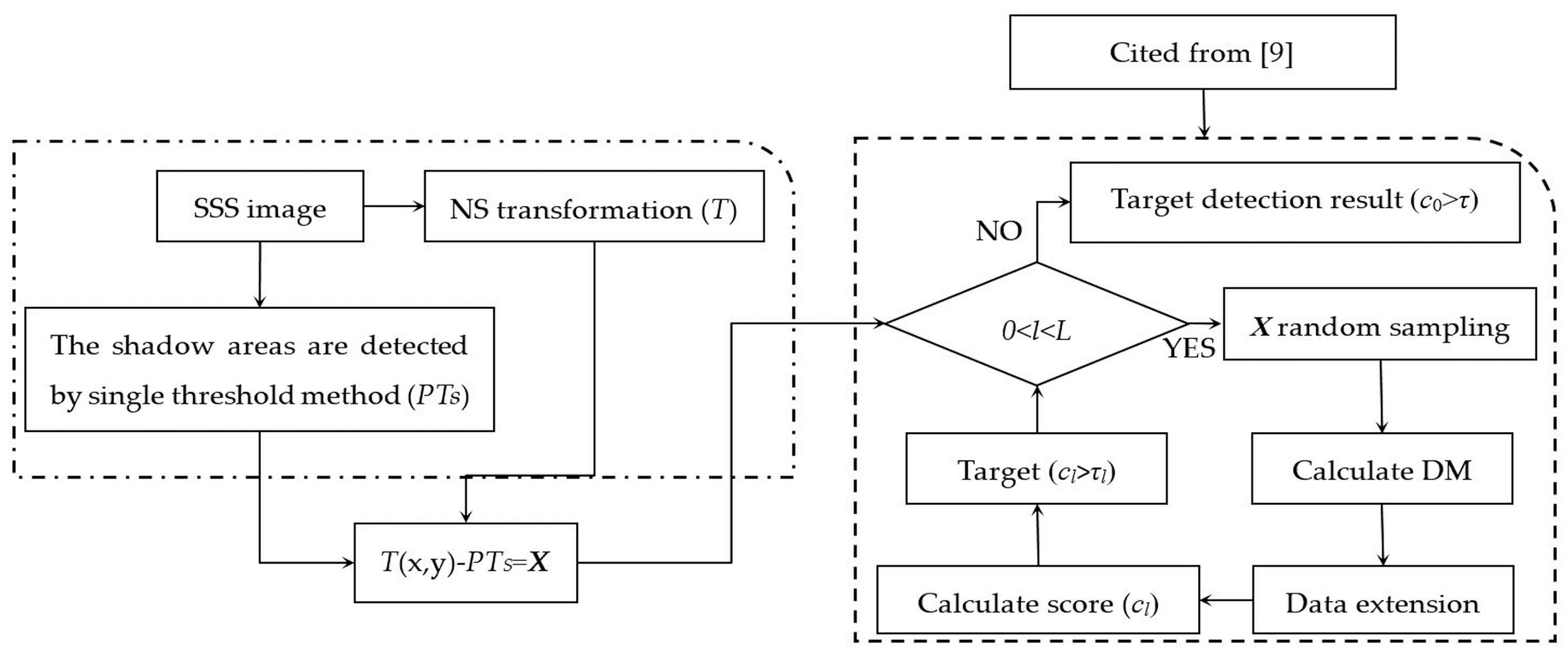
3.3. The NS + DM Algorithm for SSS Image Target Detection

Combining NS and DM, a novel target detection algorithm referred to here as NS + DM is proposed. The flow chart of the algorithm is shown in Figure 2, and the detection process is as follows.

Step 1. Transform the input SSS image into the NS domain using Equations (1)–(5) and obtain the T, I, and F subsets.

Step 2. Using the inputted raw SSS image, and considering the imaging mechanism of the shadowed areas in the SSS image with a low gray level, the single threshold method, an efficient algorithm, is recommended for the detection of the shadowed areas, and these pixels’ positions are saved as PT_s. The threshold value is obtained by calculating the image gray histogram and finding the gray level of the first wave crest. The shadowed areas are selected by finding those pixels that are less than the threshold value.

Step 3. Based on the T subset obtained by the NS transformation, the shadows’ positions saved as PT_s in Step 2 are removed from T. These residual subset pixels are labeled X. Then, X is used to calculate the diffusion map and detect the target areas.

SSS images are high-resolution; even if the image is 192 × 192 pixels, there are 36,864 data points. Calculating the DM is usually time-consuming. If the CPU is insufficiently strong, computing the DM for the entire dataset X is difficult. Therefore, to solve the problem, a DM can be constructed by using random samples of X and then by extending it to all points using the Nyström extension method [9,20].

Step 4. When the DM is constructed, and the diffusion distance provides metrics for target detection, the dissimilarity measure between two image patches can be defiened by [10]

$$c=1-exp\left\{-\frac{1}{k}{\displaystyle \sum }_{t=1}^k\frac{\raisebox{1ex}{$D\left(p_i,p_j\right)$}\!\left/ \!\raisebox{-1ex}{$2{\sigma }_k$}\right.}{1+3\times d_{position}\left(p_i,p_j\right)}\right\}$$

(13)

Equation (13) is defined as a target scoring equation, where k is the k most similar patches, d_position is the Euclidean distance between the image positions of patches p_i and p_j, D is the diffusion distance, and σ_k is the standard deviation of the distances to the kth neighbor.

In addition, considering the complex texture features of the sea bottom background image, when using Equation (13), the fractal texture feature is pulsed to c, and the fractal texture can be calculated by the fractal dimension (FD) that represents the geometrical complexity of an object. Different types of objects in the natural world generally have different FDs, and a certain correlation exists between the FD and the gray level of the image. The FD is matched for the surface roughness of the object, and the different texture images have a large difference in roughness [21]. Therefore, the fractal texture feature is useful for distinguishing artificial targets in natural sea bottom images. In the experiment, the FD was calculated using the differential box-counting method [21].

Step 5. With the aid of a mathematical morphology operation, such as open, closed, expansion, and erosion, the center contour of the targets’ areas in the input SSS image were finally obtained.

4. Experiments and Discussion

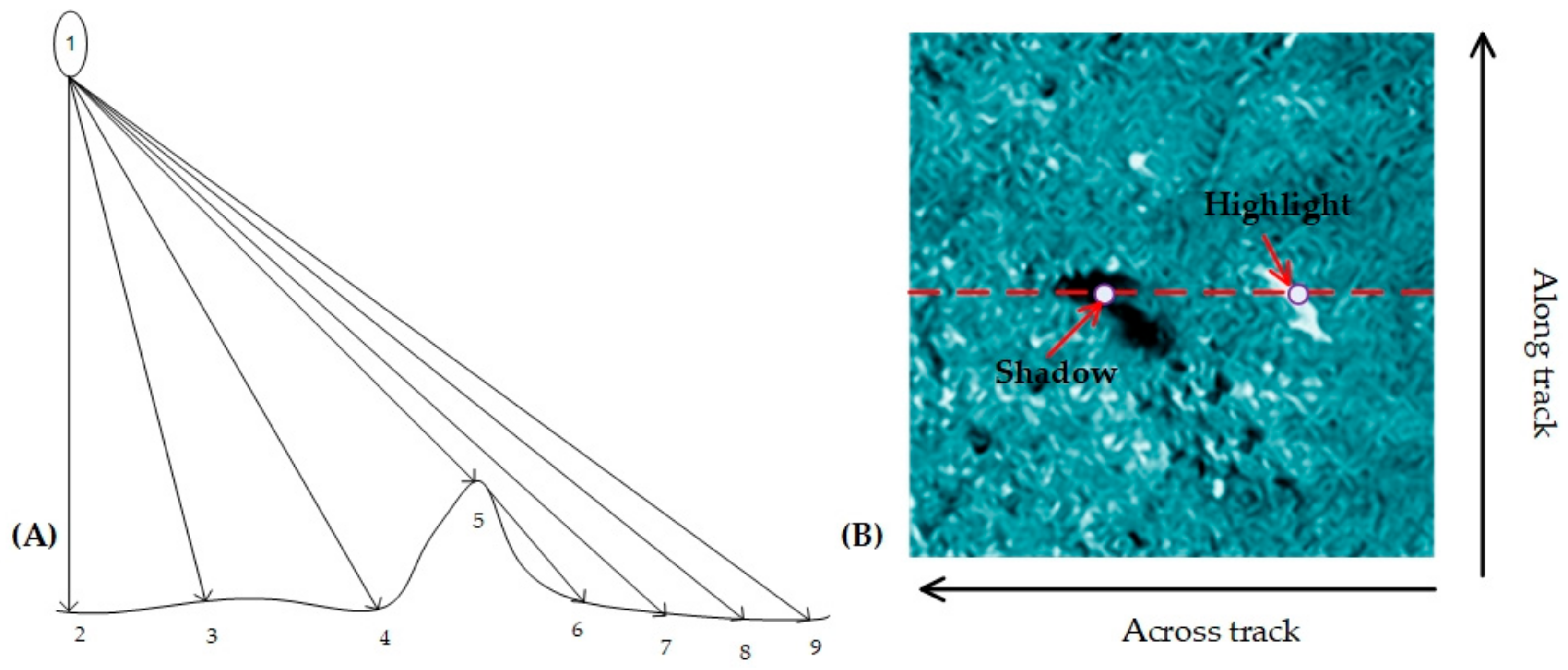
The SSS image of an obvious floating fish target with a resolution of 192 × 192 pixels shown in Figure 1B was used for the target detection experiment.

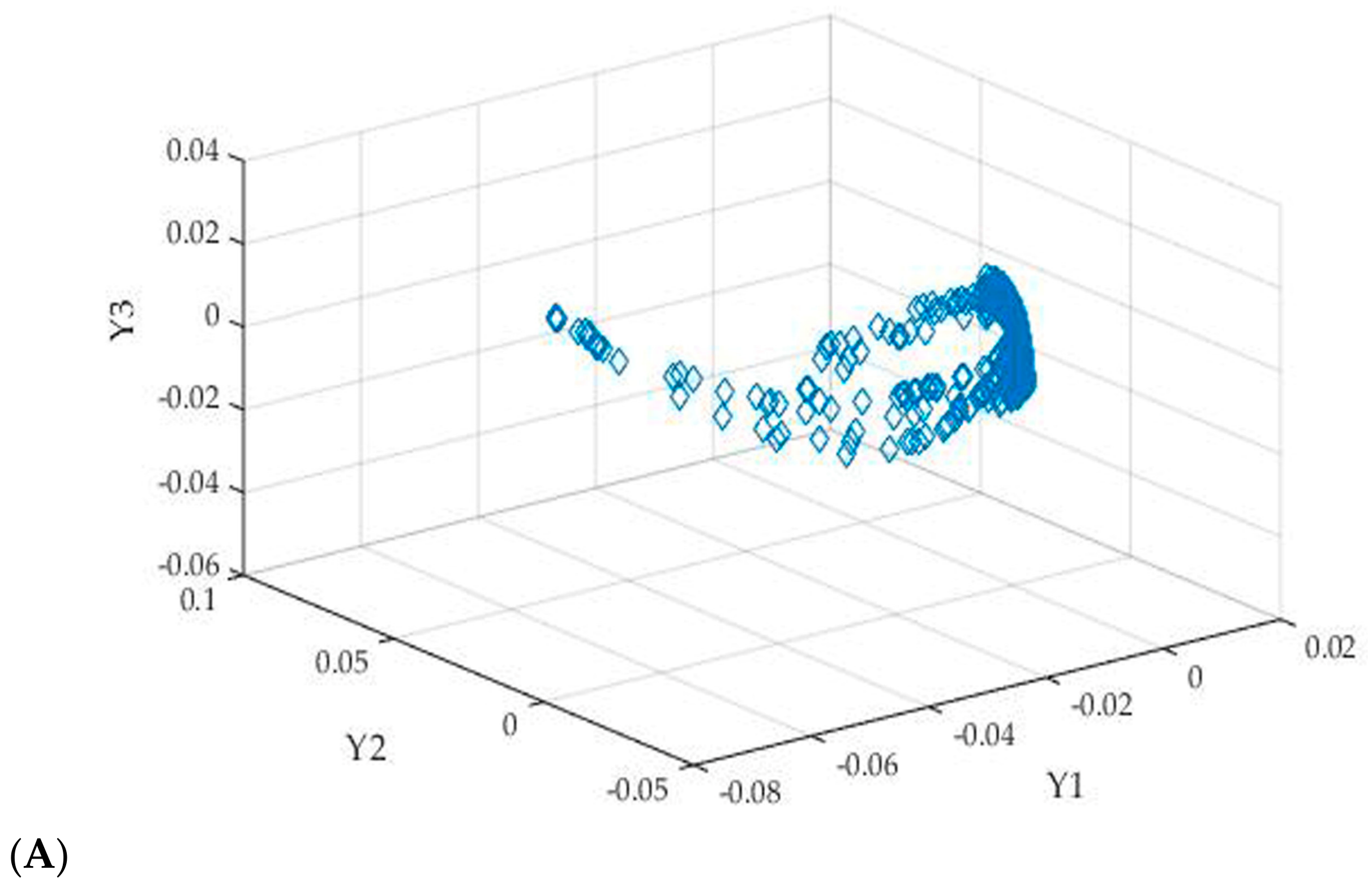
Diffusion maps are used to find a lower dimensional representation of the SSS image. For target detection, we assumed the target areas would be well separated from the background in the new embedding. In the embedding, background pixels have similar diffusion coordinates, lying in a dense neighborhood, whereas the target areas would be separated from the background and lie in a low-density neighborhood [9]. To solve the low efficiency problem in computing a diffusion map for high-resolution SSS images, a DM was constructed by using random samples of the image and then extending it to all points using the Nyström extension method as introduced in Step 4 in Section 3.3 [9,10,20]. After the DM and the out-of-sample extension were calculated, the diffusion coordinates of the diffusion map were obtained and are shown in Figure 3 and Figure 4.

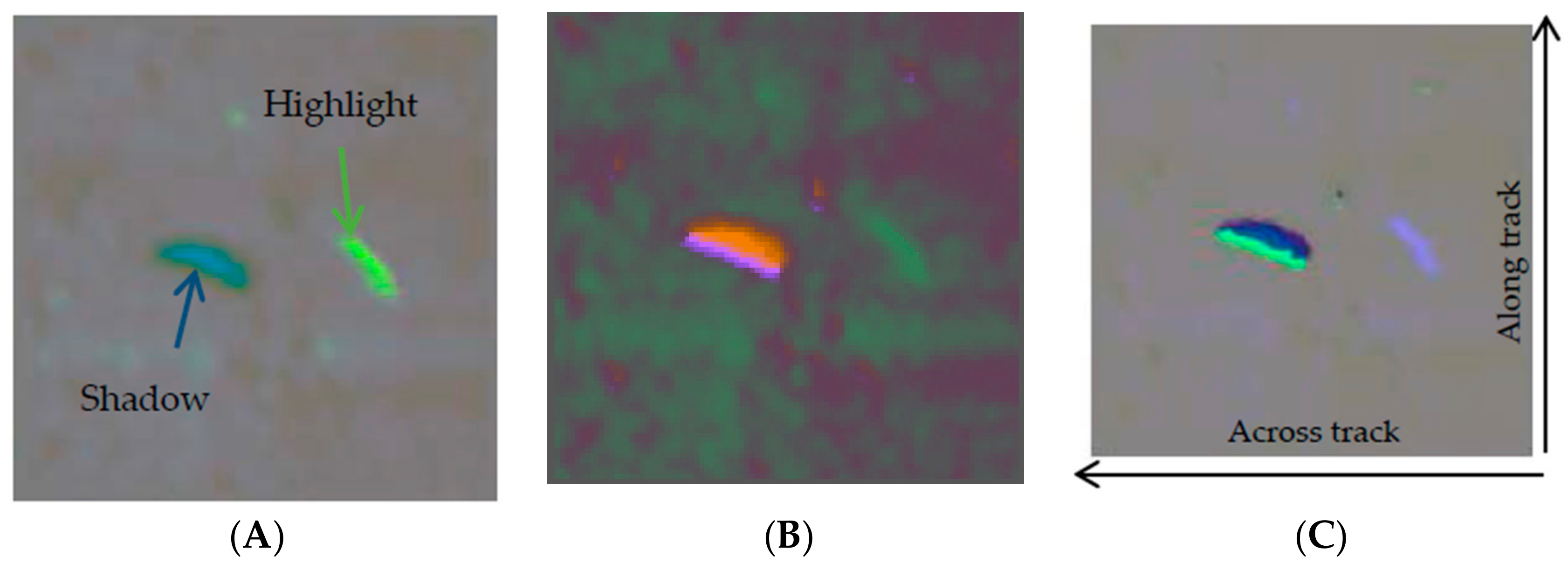
From Figure 3, the target (highlighted) areas have different colors from the background areas, which is useful for target detection. However, Figure 3 also shows that the diffusion coordinates of the shadowed areas also lie in a low-density neighborhood in the new embedding, and they are also separated from the background areas in the colored image. This characteristic will affect the accuracy of the target detection. Figure 4 further demonstrates that the diffusion coordinates in the new embedding are different in dense neighborhoods, which can be used to define the score equation for target detection, but the diffusion coordinates cannot distinguish highlighted and shadowed areas. Both Figure 3 and Figure 4 show that the anomaly areas (highlights and shadows) shape parameter change when the sampling rate decreases.

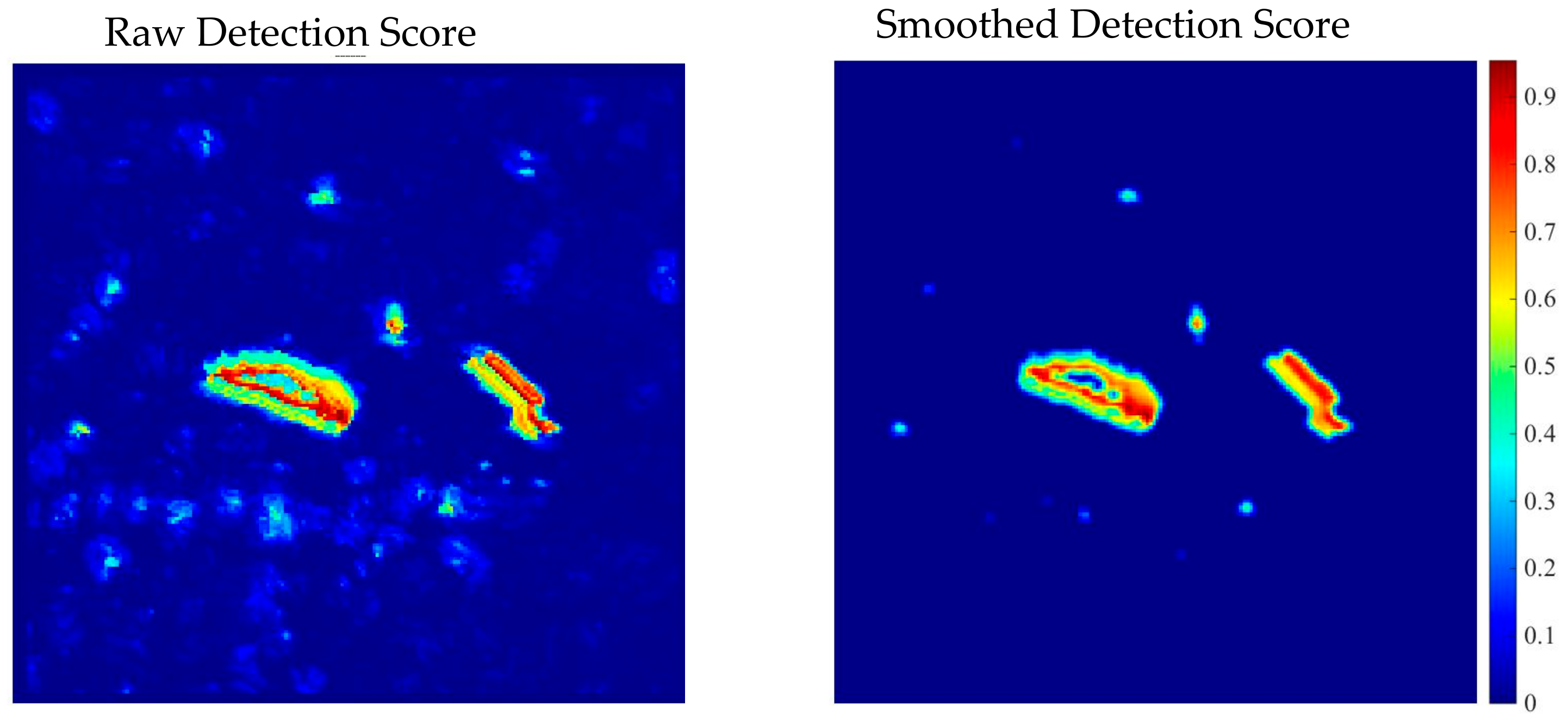
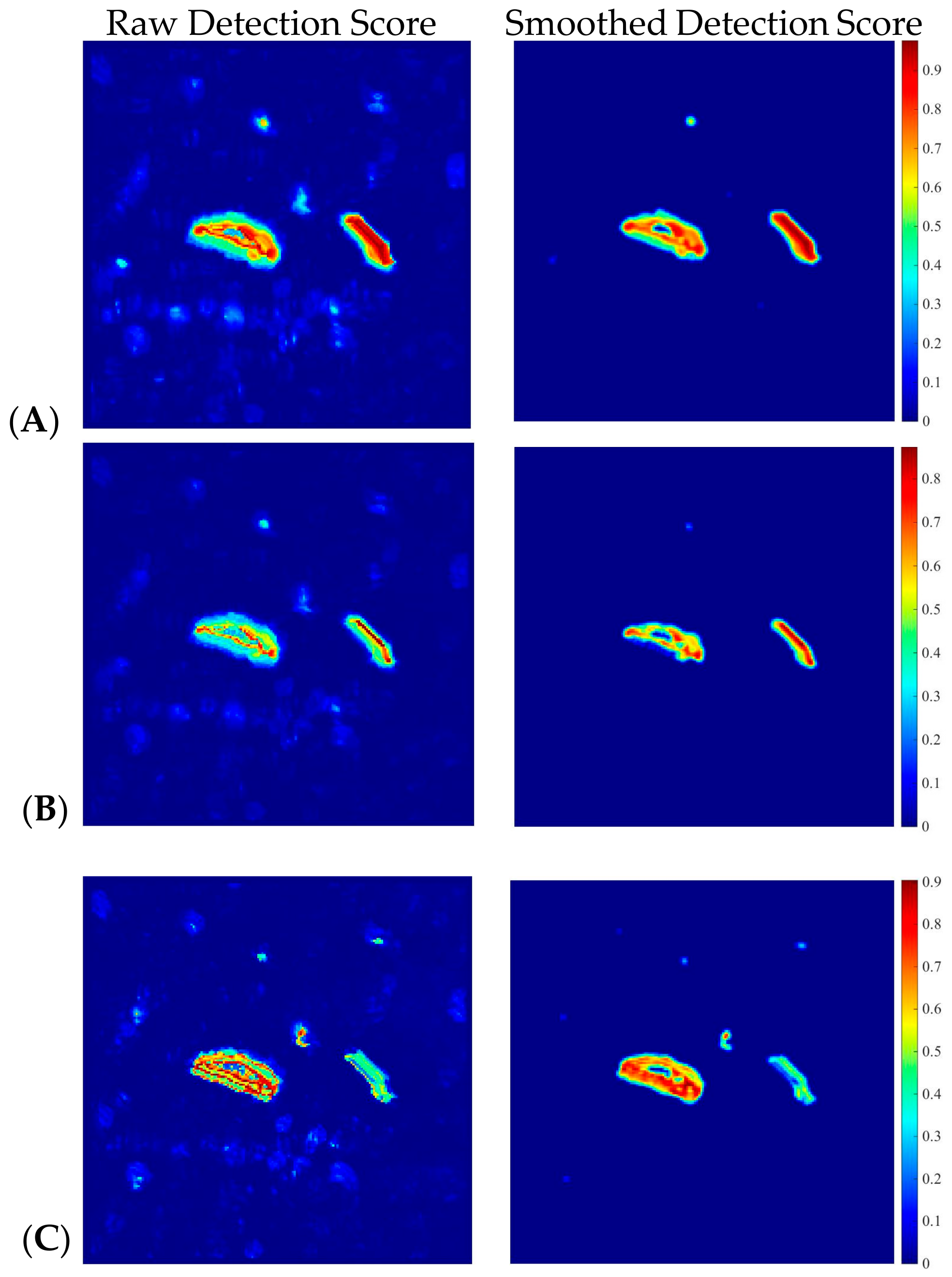
The target scoring was calculated using the equation defined in Step 4 of Section 3.3, and the parameter k used in Equation (13) was set to 64 during the calculation. The raw and smoothed target detection score are shown in Figure 5. The simple median filter was used for the smoothing process, and the filter window was defined as 5 × 5. In Figure 5, with different sample rates, the target detection score varies considerably. With the decrease in sample rate, the detection accuracy of the target contour decreases. Using the multiscale anomaly detection method [9], the method in this paper is referred to as the traditional DM method. The parameter L shown in Figure 2 is the Level of Gaussian pyramid and was set to 3 in the experiment. The target detection scores are shown in Figure 6. As can be seen in Figure 5 and Figure 6, the traditional DM can solve the problem caused when detection accuracy is influenced by using random samples. However, two additional problems influence the accuracy of target detection in the traditional DM: the influence of noises caused by the complex marine environment, and the shadowed areas. Notably, these two factors are the main characteristics of an SSS image. Therefore, we used the NS transformation to process an SSS image, and the shadowed areas were first detected before the DM was calculated. We refer here to this method as NS + DM.

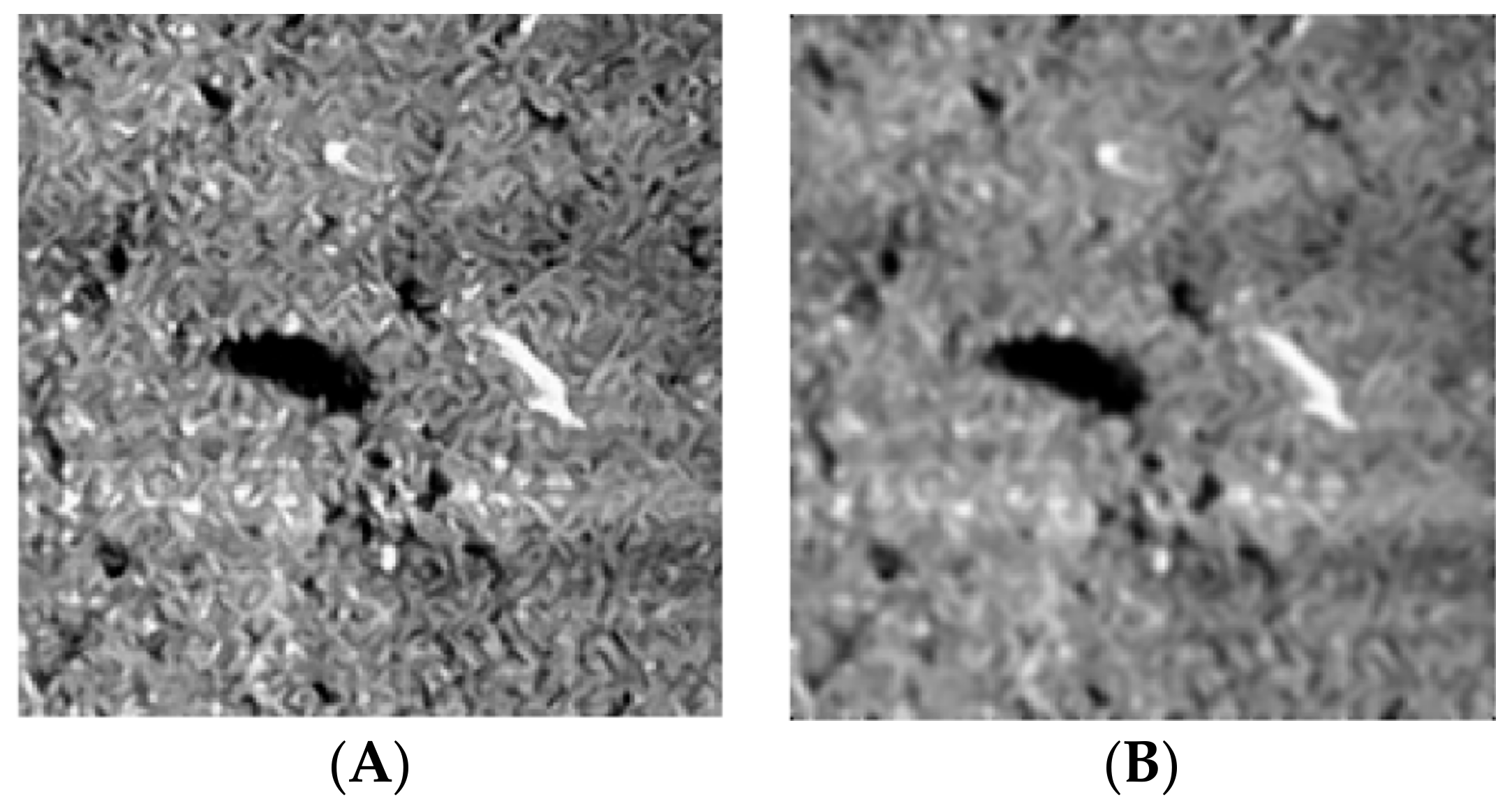
Figure 1B was first converted into a gray level image as shown in Figure 7A, and then it was transformed into the NS domain using Equations (1)–(5). The image of T_β was obtained as shown in Figure 7B. Compared with the original image, T_β contains the smooth image information due to the NS transformation process. Then, with the T_β image, the traditional DM method was applied, and the smoothed target detection score is shown in Figure 8. Comparing Figure 6 and Figure 8, the influence of the marine environment noise was removed, and only the target and shadowed areas were highlighted in the target scoring. The experiment demonstrates that the NS algorithm can reduce the variability in the SSS image and accurately detect targets from an SSS image. However, as shown in Figure 8, the shadowed areas also had a high target score and influenced the accuracy of the target detection.

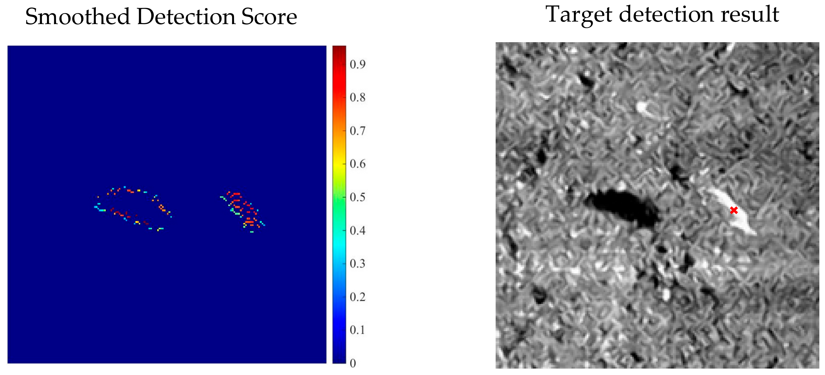
First, the shadowed areas were extracted using the threshold method; thus, in the sampling process for the DM calculation used by T_β, the shadow’s position is not always sampled. Based on the diffusion map calculated under this condition, the target score was then calculated. The smoothed target detection score and the detection result are shown in Figure 9. The target detection result is shown in the centroid of the target contour. The shadow’s edge is also highlighted when the detection score is calculated, but it is disconnected and can be easily discarded through the connected region and the contour center extracting process, which is implemented by the mathematical morphology operation. As a result, the target is accurately detected. The above experiment proved the feasibility of the proposed algorithm for an SSS image with an obvious single target.

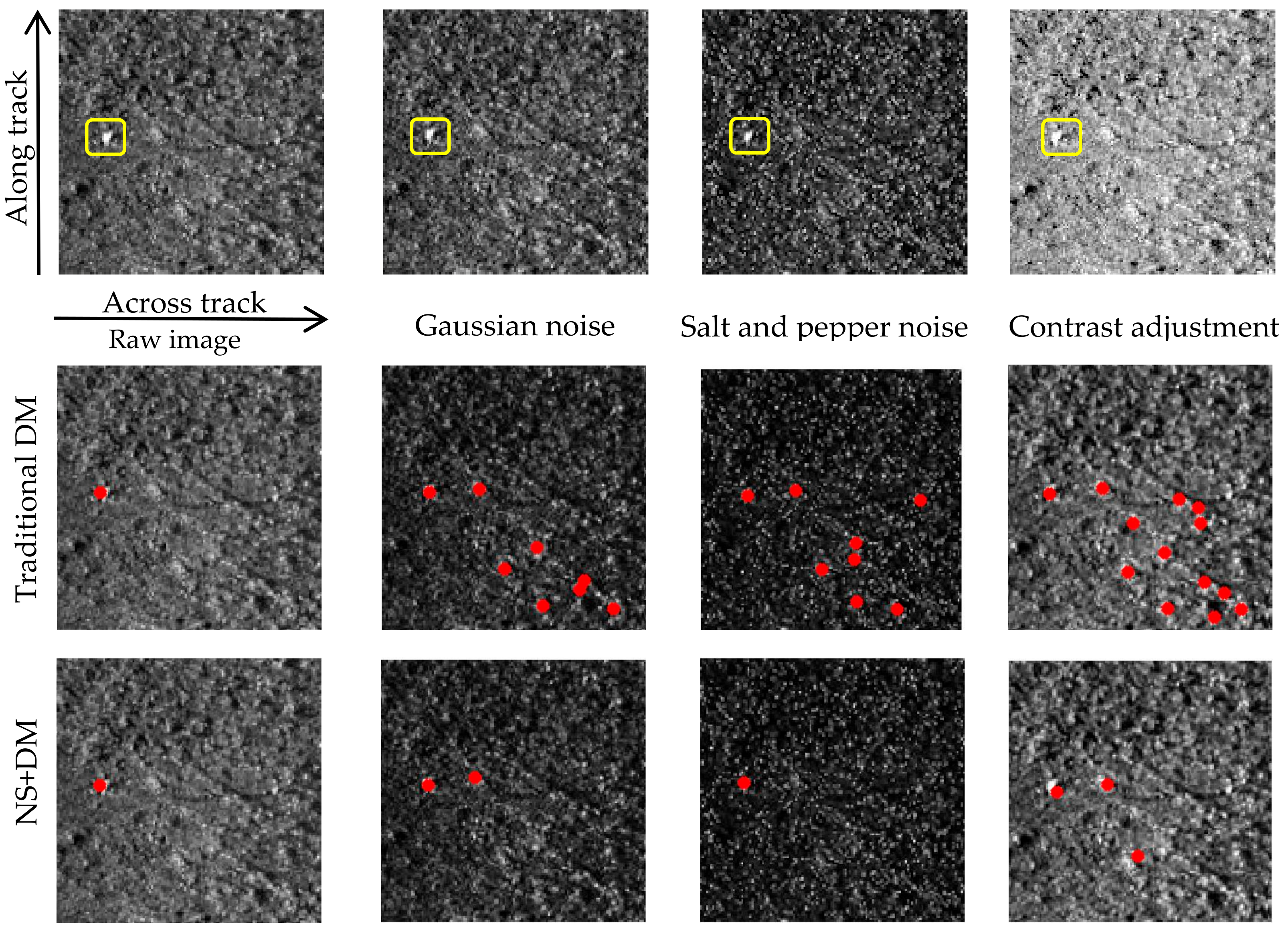
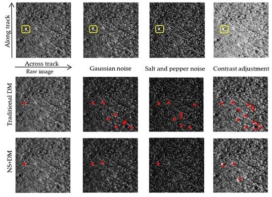
To verify the practicability of the proposed algorithm, an SSS image with complex features and an unclear target was selected for the next experiment. An SSS image is easily influenced by Gaussian and salt and pepper noises as well as radiation distortion. Therefore, the Gaussian and salt and pepper noises were respectively added to the image, and the contrast was adjusted for the experiment. The size of these images is 128 × 128 pixels. The images and the detection results are shown in Figure 10. One obvious target, a mine-like object, was detected by manual interpretation from the raw image. From Figure 10, both the traditional DM and NS + DM could accurately detect the target when no additional noise was added to the image. The traditional DM is not well suited to the handling noise and changes in image contrast and failed to detect many targets in the experiment. Conversely, the NS + DM algorithm showed good robustness to noise, and only a few missed detections occurred in the experiment. The experiment also demonstrated that, for accurate target detection in an SSS image, a pre-processing step is needed for SSS images, such as de-noising and radiation distortion correction.

These two experiments demonstrated that the proposed algorithm can accurately detect targets in SSS images with single clear or unclear targets.

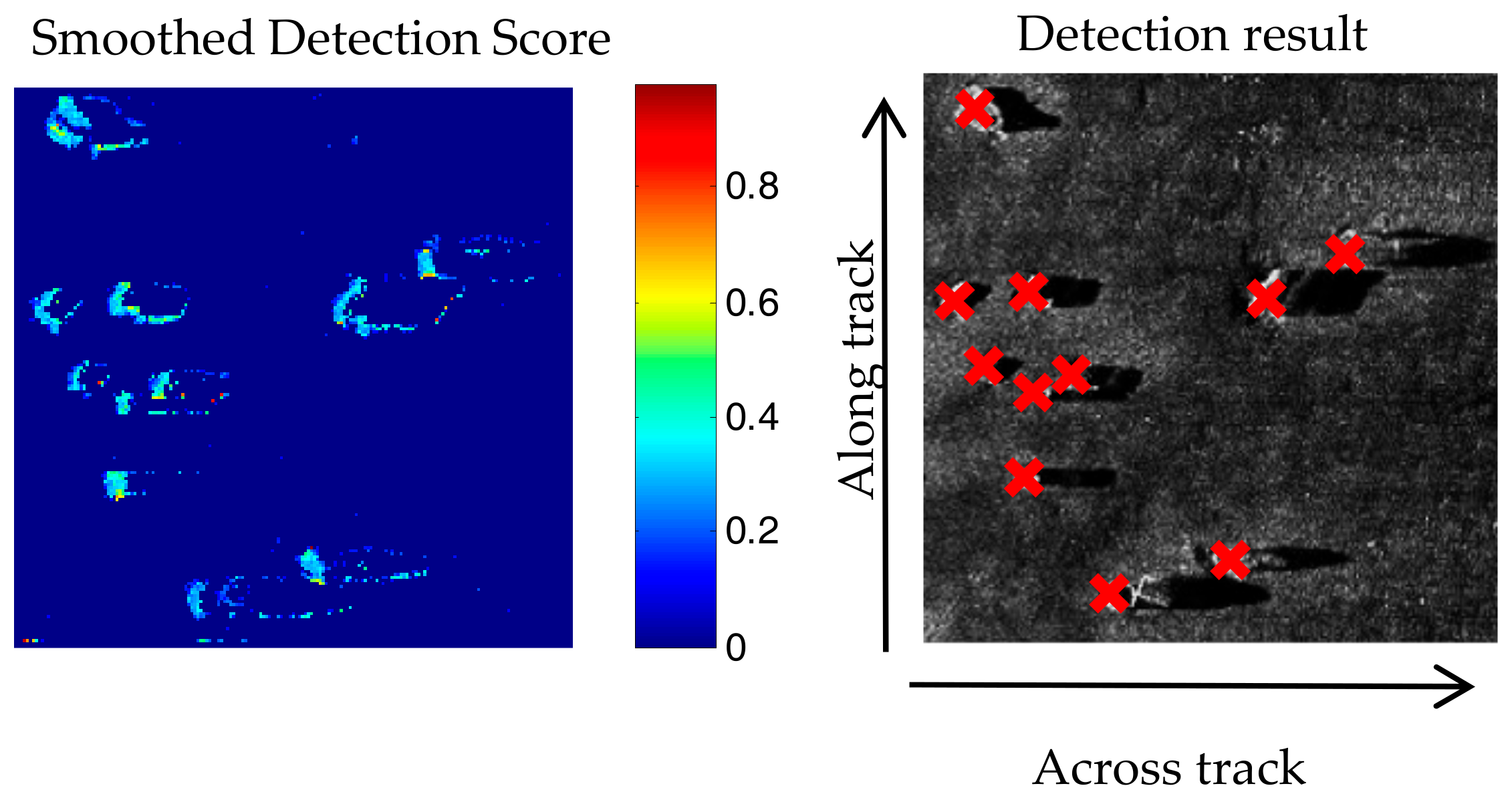
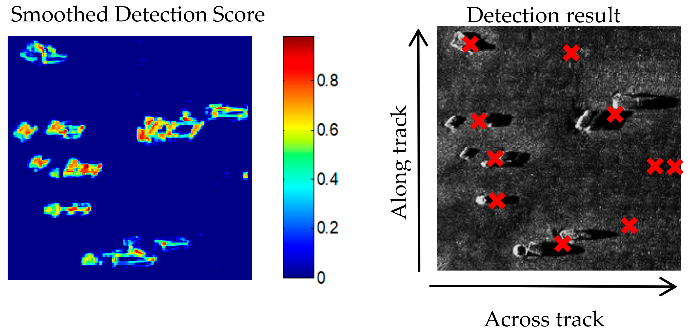
To further verify the practicability of the proposed algorithm, an SSS image with multi-targets with shadowed areas was used for a third target detection experiment. The detection results are shown in Figure 11 and Figure 12. Using the traditional DM method, 10 targets were detected, with two false detections and three missing detections. Eleven targets were detected by the NS + DM algorithm, with no false or missing detections.

Because the shadowed areas always follow behind the highlighted area in an SSS image, especially when the target is on the sea bottom, the diffusion coordinates of these shadowed areas are also different from the background areas. The shadow detection score was very high when calculating the target score. Also, being influenced by waves, currents, and other disturbances, noise always accompanies an SSS image, and result in the blurring of the target image. These characteristics mean accurately detecting multiple targets from an SSS image with shadowed areas using the traditional DM method is difficult. After NS transformation and considering the shadowed areas, the noise was partially eliminated after the NS operation, regardless of the position of the shadows’ areas in calculating DM. Although the shadows’ edge had a high detection score, it was discontinuous and would be discarded by the mathematical morphology operation, enabling the accurate detection of multiple targets with shadowed areas in an SSS image.

Finally, an SSS image with multiple targets with no obvious shadows was used for the fourth target detection experiment. The detection results are shown in Figure 13. NS + DM also accurately detected targets with no false or missing detections. The traditional DM had one false and two missing detections because the image was influenced by complex marine noise.

These two experiments demonstrated that the proposed algorithm can accurately detect targets in SSS images for multiple targets.

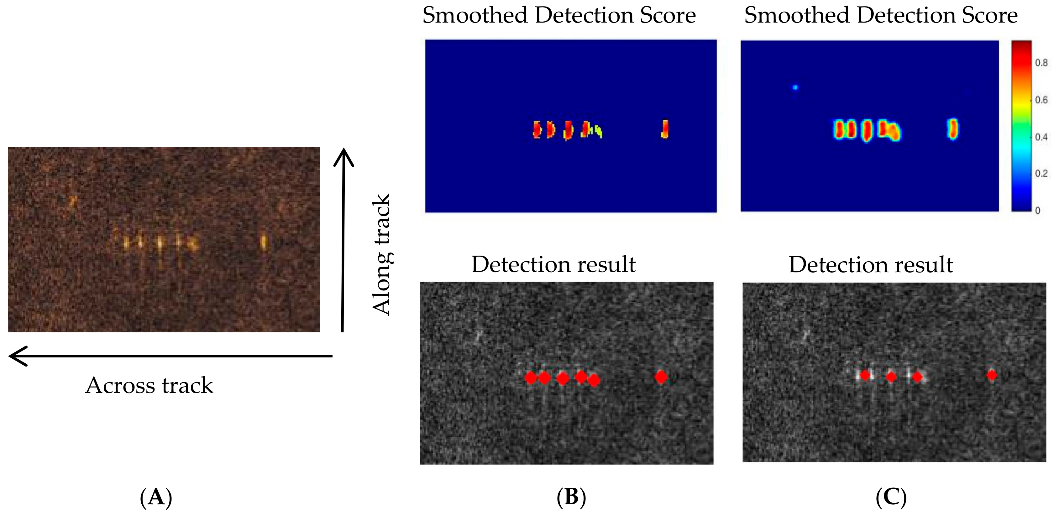
In the introduction, we mentioned that the accurate target detection with SSS images of sand wave terrain is complex. To further evaluate the NS + DM algorithm, we compared it with the methods mentioned in the introduction to detect targets in SSS images of sand wave terrain.

The real SSS measurements were conducted in the Nanhai Sea in China where sand terrain is significant. A dual-frequency Edgetech 4200 MP SSS system with a low frequency of 125 kHz and a high frequency of 425 kHz was used in the SSS measurement. During the data acquisition, the towed operation was used, the slant range of 125 m was set, and the Ping sample rate for the low and high band was 7234 and 10,848, respectively. With the help of the developed software [23], the raw SSS XTF (eXtended Triton Format) files were first decoded, and the low frequency (125 kHz) data were extracted for the experiment. As the raw backscatter data ranged between 0 and 32,767 (16 bit quantization), we re-quantized these backscatter data to 8-bit using the Bell μ-law proposed by Blondel [24]. In the image formation process, the resolution of the waterfall image was set to 0.6 m. To maintain the consistency of the resolution along and across the track, the ship speed correction was also completed. The SSS image was significantly influenced by the sound attenuation and the diffusion with the sound transmission distance and water properties. 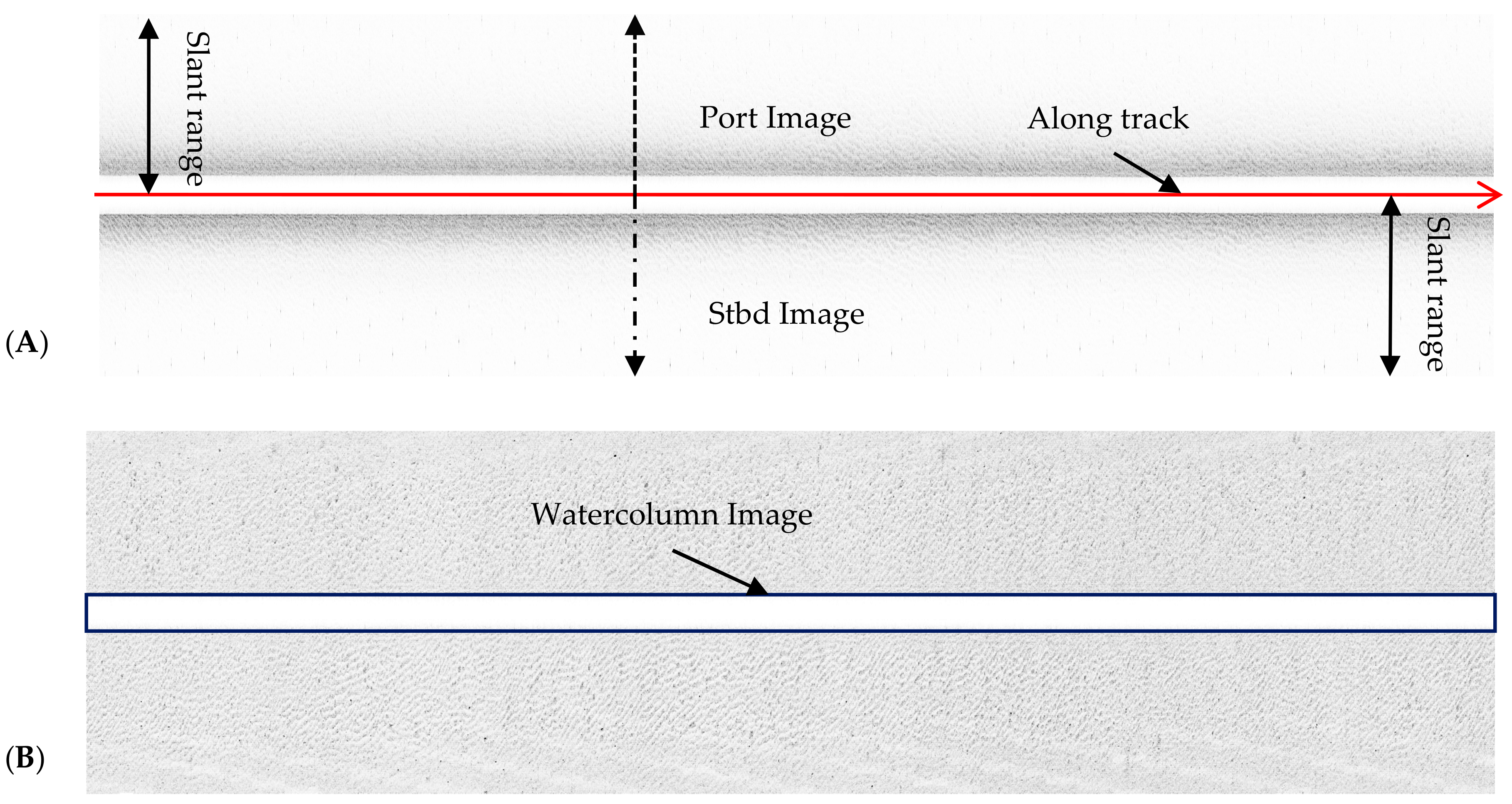Before the target detection process, the time vary gain (TVG) and radiation distortion correction were processed for the SSS image [25,26]. Single strips of a raw SSS image and a corrected image are shown in Figure 14. Both images were 4226 × 250 m. Figure 14A shows the raw SSS image, showing that the image is significantly influenced by sound attenuation and diffusion as the slant range increases. Figure 14B shows the corrected image, and the image’s gray level is balanced both along and across the track.

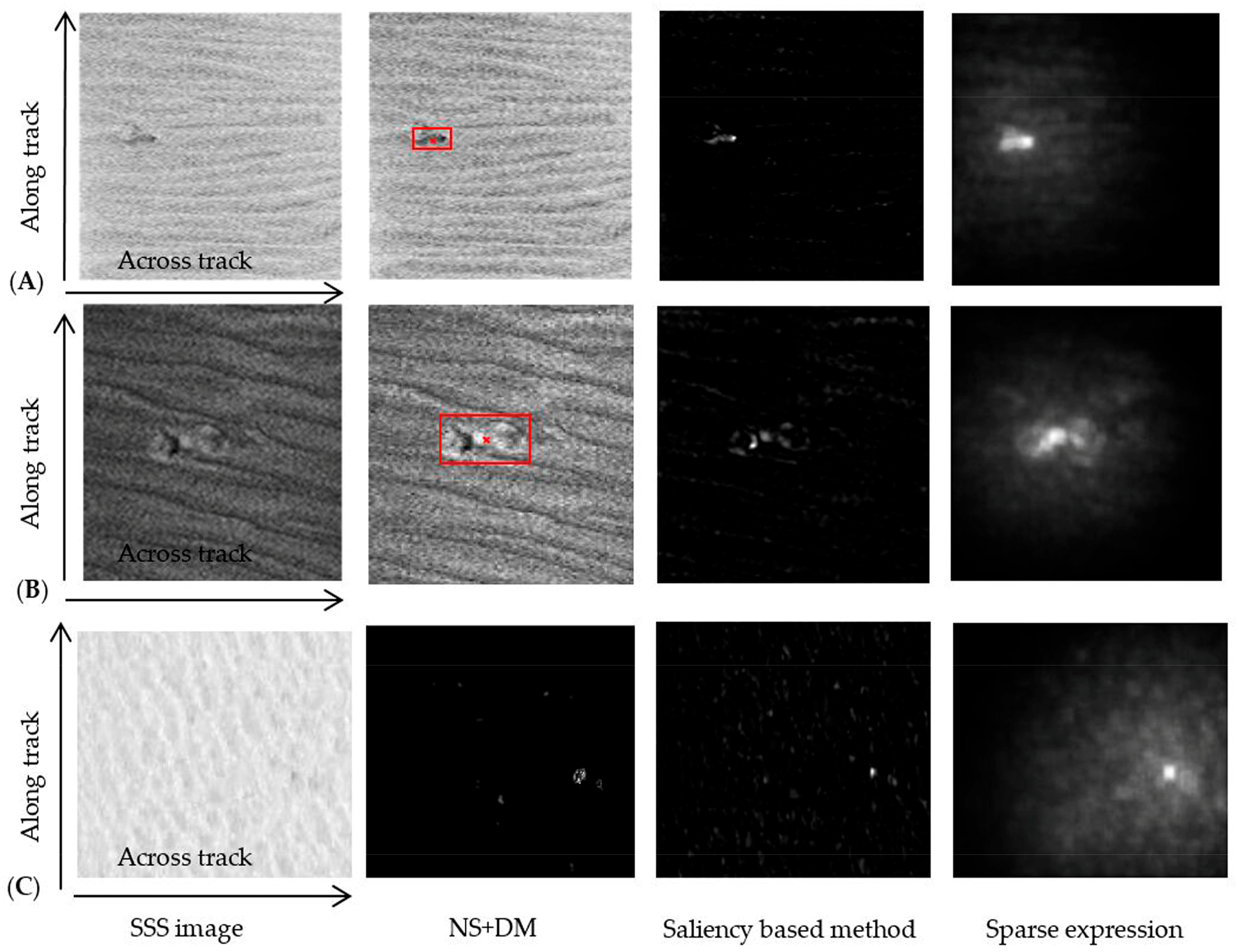
The partial image was intercepted from the entire waterfall image in different strips to complete the target detection experiments and their detection results are shown in Figure 15. Modeling the sand wave terrain textures and the shape feature for different targets with fixed parameters is difficult, so the statistical model and matching template-based methods were not used in the experiments. As can be seen in Figure 15A,B, NS + DM can accurately detect the target in an SSS image of sand wave terrain. In the detection results based on the saliency and the sparse representation methods [27,28], the value of the raised surface of the sand wave and the target of the binary image was mostly one, whereas the value of the background image was zero. The target areas were not accurately extracted, and its contour center could not be determined. That is, the target was not accurately detected. The reason for the target detection failure with the saliency-based method occurred because the provided saliency criterion could not accurately match the background and target areas of the sand wave terrain texture. The reason for the sparse representations was mainly because the dictionary-learning model of the sand wave texture was not accurate. Figure 15C shows an SSS image with no target in the sand wave terrain. In the target detection process, no target was detected by the NS + DM algorithm, and the target detection score was calculated (Figure 15C). Although some highlighted areas were found in the image, the score was very low, with the highest value being 0.16. When the right τ_l is given, some lower values were filtered as zero, and the remaining values included some scattered ones. The values were disconnected, and the targets’ centers could not be obtained. As can be seen in Figure 15C, the two other methods encountered the same problems as those indicated by Figure 15A,B. The NS + DM algorithm did not require the training samples, and no parameter estimates were required, providing an effective method of accurately detecting targets in SSS images. All of the above experiments verified the effectiveness of the NS + DM algorithm.

5. Conclusions

The main contribution of this paper is the novel SSS image target detection algorithm integrating an NS and a DM. In the algorithm, the SSS image was first transformed into the NS domain, and the subset of T_β can be seen as the de-noised image with high contrast, which is beneficial for improving the accuracy of the SSS image target detection. To further improve the accuracy, considering the imaging mechanism of the shadowed areas in SSS images with a low gray level, the single threshold method, an efficient algorithm, was used to remove the shadowed areas. When the DM was calculated, the position of the shadowed areas was not sampled, and the traditional DM method was then used to detect the target in an SSS image using the improved target scoring equation. Experimental results showed that the proposed algorithm improves the target detection accuracy for SSS images in different sea bottom sediments with different targets.