Abstract
In the dwindling natural mangrove today, mangrove reforestation projects are conducted worldwide to prevent further losses. Due to monoculture and the low survival rate of artificial mangroves, it is necessary to pay attention to mapping and monitoring them dynamically. Remote sensing techniques have been widely used to map mangrove forests due to their capacity for large-scale, accurate, efficient, and repetitive monitoring. This study evaluated the capability of a 0.5-m Pléiades-1 in classifying artificial mangrove species using both pixel-based and object-based classification schemes. For comparison, three machine learning algorithms—decision tree (DT), support vector machine (SVM), and random forest (RF)—were used as the classifiers in the pixel-based and object-based classification procedure. The results showed that both the pixel-based and object-based approaches could recognize the major discriminations between the four major artificial mangrove species. However, the object-based method had a better overall accuracy than the pixel-based method on average. For pixel-based image analysis, SVM produced the highest overall accuracy (79.63%); for object-based image analysis, RF could achieve the highest overall accuracy (82.40%), and it was also the best machine learning algorithm for classifying artificial mangroves. The patches produced by object-based image analysis approaches presented a more generalized appearance and could contiguously depict mangrove species communities. When the same machine learning algorithms were compared by McNemar’s test, a statistically significant difference in overall classification accuracy between the pixel-based and object-based classifications only existed in the RF algorithm. Regarding species, monoculture and dominant mangrove species Sonneratia apetala group 1 (SA1) as well as partly mixed and regular shape mangrove species Hibiscus tiliaceus (HT) could well be identified. However, for complex and easily-confused mangrove species Sonneratia apetala group 2 (SA2) and other occasionally presented mangroves species (OT), only major distributions could be extracted, with an accuracy of about two-thirds. This study demonstrated that more than 80% of artificial mangroves species distribution could be mapped.
1. Introduction
Mangroves are salt-tolerant evergreen woody plants, distributed in the inter-tidal region in tropical and subtropical regions [1]. They provide breeding and nursing grounds for marine and pelagic species and play an important role in windbreak, shoreline stabilization, purification of coastal water quality, carbon sequestration, and maintenance of ecological balance and biodiversity [2]. During the past 50–60 years, mangrove forests in China have been largely reduced from 420 km2; in the 1950s to 220 km2 in 2000 due to agricultural land reclamation, urban development, industrialization, and aquaculture [3]. However, in the past 20 years, with the increasing efforts in environmental protection from the Chinese government, artificial mangroves have been widely planted in China [4,5]. Artificial mangrove forests are designed and planted artificially (such as by artificially breeding seeds, modifying the topography and components of the ground, and changing the distance between plants) according to people’s needs, imitating the components of natural mangrove wetlands and planted in some certain geographical locations. Artificial mangroves have the characteristics of monoculture and low survival rates.
In order to understand the regeneration and expansion capability of artificial mangrove forests and provide species distribution data for mangrove reforestation, it is important to classify and map these artificial mangrove forests. Since mangrove forests are dense and located in intertidal zones and always inundated by periodic seawater, it is very difficult to access mangrove forests for the purpose of extensive field surviving and sampling. Therefore, remote sensing data have been widely used in mangrove mapping. Various remote sensing data have been used in mangrove forests research, ranging from high resolution aerial photos to middle and high resolution satellite imagery, and from the hyper-spectral data to the synthetic aperture radar (SAR) and light detection and ranging (LiDAR) data [6]. Pléiades-1 images, however, have been rarely used for mangrove forest mapping and classifying and should be able to map mangrove features due to their very high spatial resolution [7,8]. The classification of mangroves from remote sensing images can be divided into two general image analysis approaches: (1) classification based on pixels; and (2) classifications based on objects.
Previously, pixel-based approaches were frequently used to identify mangrove distribution. This may be caused by the coarse spatial resolutions of traditional remote sensing images before the launch of satellites equipped with high-resolution sensors. Kanniah et al. (2007) [9] found that the pixel-based maximum likelihood classification (MLC) using 4-m IKONOS data with corresponding texture information could achieve an 82% overall accuracy in mangrove species classification. Wang et al. (2008) [10] showed that clustering-based neural network classification utilizing 4-m IKONOS imagery with textural information from the panchromatic band could obtain an 0.93 Kappa value for discriminating mangrove species. Neukermans et al. (2008) [11] found that the pixel-based fuzzy classification using pan-sharpened QuickBird imagery could produce a 72% overall accuracy for the detection of mangrove species. Object-based approaches have been frequently applied for mapping mangrove species in recent years. For example, using QuickBird and IKONOS data, Wang et al. (2004) [12] utilized an object-based MLC algorithm to classify mangroves and found that overall classification accuracies were less than 76%. Kamal et al. (2015) [13] showed that the standard nearest neighbor (NN) algorithm using 0.5-m WorldView-2 imagery only achieved an overall classification accuracy of 54% for demarcating mangrove species communities.
For algorithm comparisons between pixel-based and object-based classifications, Wang et al. (2004) [14] contrasted a pixel-based MLC classification with an object-based NN classification on mangrove species mapping using IKONOS images and indicated that a hybrid object-based method achieved the highest classification accuracy (91.4%). Myint et al. (2008) [15] compared a pixel-based MLC algorithm with an object-based NN algorithm when extracting three mangrove species and surrounding land use classes using a Landsat TM image. Their results showed that object-based approaches outperformed traditional pixel-based methods with an overall accuracy greater than 90%. Kamal et al. (2011) [16], employing hyper-spectral CASI-2 (compact airborne spectrographic imager 2) data, made a comparison between a pixel-based spectral angle mapper, a pixel-based linear spectral unmixing, and an object-based NN classification method for distinguishing three mangrove species and surrounding land use types. They found that the object-based classification using an NN algorithm was more accurate than pixel-based methods with an overall accuracy greater than 75%.
In general, the above comparisons demonstrated that object-based methods were superior to pixel-based methods for mangrove species classifications, especially using high-spatial-resolution satellite images. However, unlike previous comparisons of pixel-based or object-based algorithms in isolation, many studies have employed relatively simple classification algorithms such as object-based classification using the NN algorithm and pixel-based classification using the MLC algorithm. Furthermore, the MLC is a probabilistic-based algorithm and is less suited to datasets that are multi-modal and non-normally distributed [10]. It is necessary to examine the performances of pixel-based and object-based classifications in mangrove species classification with relatively modern and robust algorithms such as the support vector machine (SVM) and random forest (RF). SVM has been used in mangrove remote sensing in recent years and performs well [17,18,19]. As a classic machine learning algorithm, decision tree (DT), referred to as CART (classification and regression tree) or C4.5 algorithm et al., is less used in mangrove classification. RF is a relatively new technique for mangrove species mapping, though it has been widely applied in land [20,21] and plant species [8,22] classification with different sensors in recent years. In addition, DT, RF and SVM all can be implemented in eCognition 9.0 (a popular object–based image analysis software, Trimble, Sunnyvale, CO, USA) with streamlined production models. Therefore, we selected these three algorithms.
The mangrove forests of Nansha Wetland are a typical artificial mangrove forest in China, consisting of a large number of Sonneratia apetala (a fast-growing, high survival rate, and exotic mangrove species). Against this background, the present study aimed to compare pixel-based and object-based image analysis approaches with selected modern and robust machine learning algorithms for the classification of artificial mangroves at a species community level using very high spatial resolution imagery in a typical artificial mangrove site in Guangdong. Three specific objectives were addressed:
- (1)
- To apply DT, SVM, and RF algorithms for both pixel-based and object-based classifications to distinguish species communities of artificial mangroves;
- (2)
- To conduct a visual assessment of the classification thematic maps and statistically compare pixel-based and object-based classifications; and
- (3)
- To assess the influences of pixel-based and object-based classifications on thematic maps from the landscape pattern perspective.
2. Data and Methods
2.1. Study Area
The Nansha Wetland (centered at latitude 22°36′ N and longitude 113°38′ E) is located in Lingding Bay of the Pearl River Estuary, Guangdong, China, covering an area of approximately 656 ha (Figure 1). As a typical tropical–subtropical wetland ecosystem in the Pearl River Estuary, the Nansha Wetland is the largest conservation area for artificial mangroves in Guangzhou city, China. The artificial mangroves Sonneratia apetala and Hibiscus tiliaceus are the dominant vegetation species with other mangroves, phragmites, banyan tree, lotus and grass occasionally presented. The place of Nansha Wetland was originally an estuary mudflat, so the terrain is still very flat. This region belongs to the subtropical monsoon climate, and the annual average temperature is 21.8 °C, and the average annual rainfall is 1635.6 mm.
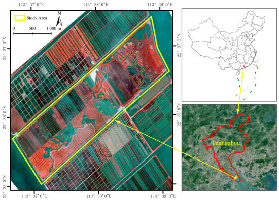
Figure 1.
The location and false color combination of Pléiades-1 data of the study area (Coordinate system: Universal Transverse Mercator Zone 49N, WGS84).
2.2. Field Survey
Field data were collected during March to May 2014 in the Nansha Wetland, which was not consistent with the remotely sensed time of the imagery employed (22 September 2012). However, the field data were still valid and could be used as training and validating samples for classification, as the community composition of Nansha has not experienced any large changes since that time, according to consultation with staff at the park. The staff stated that there was no record of any natural or human disturbances that could devastate the mangroves during this period. In addition, if the planted mangroves died, they would replant the same mangrove species in the same places.
We collected a total of 219 field samples. A sample was defined as a homogeneous patch of at least 25 m2, which is at least 100 pixels in the Pléiades-1 image. The shape of the sample is circular or approximately square. These field samples were obtained through the random sampling technique along almost all the accessible riverways of the Nansha Wetland and covered most of the study area to ensure all of the mangrove species represented. At the same time, we used Google Earth for mobile with an assisted global positioning system (A-GPS) to record the coordinates of each mangrove sample and available species. In any case, all samples were selected from sites that were located away from the edges and where no community composition changes had occurred to avoid any errors in classification due to natural growth, regeneration, or vegetation decline.
Through our investigations, there are 17 kinds of replanted mangroves in the Nansha Wetland, of which 10 types are true mangroves and seven types are semi-mangroves [23]. Sonneratia apetala and Hibiscus tiliaceus were the dominant species of the north and south, respectively, and accounted for nearly 80% of the total mangrove area [24,25]. Based on community structures and tree characters, Sonneratia apetala can be divided into two kinds: Sonneratia apetala group 1 (SA1), and Sonneratia apetala group 2 (SA2). SA1 is a mature and pure species community; SA2 is a young community partially mixed with other species. Thus, the 17 species were divided into four groups: SA1, SA2, HT (Hibiscus tiliaceus), and OT (other mangroves).
All samples were divided into two sets based on their spatial distribution, with one set designated for training the classifier and the other for assessing classification accuracy (Figure 2). The number of training and validating samples collected in the field for each mangrove species is shown in Table 1.
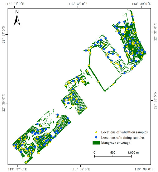
Figure 2.
The location of field samples available for training and validation purposes.

Table 1.
Number of training and validating samples for each mangrove species.
2.3. Remote Sensing Data and Pre-Processing
The Pléiades-1 (Pléiades-1A, launched on December 2011) images of Nansha consisted of one panchromatic image at 0.5-m resolution and one multispectral image at 2-m resolution, which were acquired on 22 September 2012. The multispectral image provided four bands: blue, green, red, and near infrared. The Pléiades-1 images were radiometrically corrected. First, digital numbers were converted to at-sensor radiance values. Second, the radiance value was converted to surface reflectance using the FLAASH (fast line-of-sight atmospheric analysis of the spectral hypercubes) model in ENVI 5.3 (Harris Geospatial, Melbourne, FL, USA). Finally, the Gram–Schmidt spectral sharpening method was used to fuse the 0.5-m panchromatic image and 2-m multispectral image to produce a 0.5-m pan-sharpened image [26].
2.4. Feature Selection, Mangroves Classification, and Image Segmentation
Mangroves were classified with a three-level hierarchy model. The first level discriminated vegetation and non-vegetation; the second level separated mangroves and non-mangroves within the vegetation class and generated a mask of mangroves; and the third level demarcated four mangrove species groups using either pixel-based or object-based classification within the mangrove class image (Figure 3). Level 1 and Level 2 were processed using the object-based image analysis method.
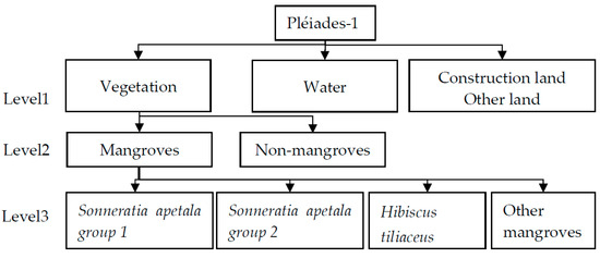
Figure 3.
The three-level hierarchy model of mangroves classification.
The object-based image analysis is based on segmentation, which can divide the image into ecologically significant, spatially continuous, and spectrally homogeneous objects or pixel groups [18]. Image segmentation was processed in eCogniton Developer 9.0 using the multi-resolution segmentation (MRS) algorithm, which is a very popular segmentation algorithm for land use and mangrove classification [17,20,27,28,29]. MRS is a “bottom-up” merging approach, which begins with pixel-sized objects and iteratively grows to merge small objects into a larger one until the homogeneous threshold of the image object is exceeded. The homogeneous threshold is determined by user-defined parameters such as scale, color/shape, compactness/smoothness, and image layer weights, of which scale is the most important parameter, directly controlling the size of image objects. Usually, an appropriate segmentation is that each object visually corresponds to the outline of a real-world individual entity of interest [18,20]. In this research, we tested a serial of scale parameters and other parameters from high to low until a satisfactory match between image objects and landscape features of the study area was achieved. Consequently, the segmentation parameters were set as follows: scale (200), color (0.9), shape (0.1), compactness (0.5), and smoothness (0.5).
At Level 1, as normalized difference water index (NDWI) values greater than or equal to zero represent all types of water features, NDWI was introduced as a threshold value to extract water [30].
NDWI = (Green − NIR)/(Green + NIR),
Due to some normalized difference vegetation index (NDVI) values of soil overlapping with vegetation and the brightness of the soils being greater than the vegetation, the brightness values were used with NDVI to separate vegetation from soil and others, that is, two threshold conditions are satisfied at the same time. The remaining objects at Level 1 were classified as “construction–other land” (including building, roads, soil and mudflats).
where is the brightness of object v, is the brightness weight of image layer k with ; K is the number of image layer k used for calculation; w is the sum of brightness weights of all image layers; is mean intensity of image layer k of image object v.
NDVI = (NIR − R)/(NIR + R),
At Level 2, for high resolution images, NIR and red bands were found useful for separating mangroves from non-mangroves [13]. As the ratio of the length to width of non-mangrove objects was higher than the mean ratio of the length to width of mangrove objects, the ratio combined with the NIR mean was introduced as a threshold value for extracting mangroves. In addition, the extracted mangrove objects were examined and manually edited, which produced a precise mask of mangrove forests.
At Level 3, the mangrove species classifications were performed within the mask of mangrove forests. Before classification, the features were selected for object-based and pixel-based classifications, individually, based on past experience and user knowledge or some feature selection algorithms [12,31]. For object-based classification, three kinds of object features were selected: spectral features, geometry features, and texture features. Spectral features were the mean value of R/G/B/NIR/Brightness and NDVI. Geometry features were the shape index. Texture features were contrast, entropy, and correlation (at four directions from a gray level co-occurrence matrix (GLCM) after Haralick). The texture values of objects were calculated based on the mean value of four layers (R/G/B/NIR). For pixel-based image classification, we selected four bands of Pléiades-1 pan-sharpened imagery and the NDVI layer, and calculated the texture of contrast, entropy, and correlation for the five layers using the “co-occurrence measures” tool in ENVI 5.3. Finally, the total number of variables used in pixel-based classification was 20, which was approximately equal to that of object-based classification (19).
2.5. Tuning of Machine Learning Algorithm Parameters
The parameter tuning and algorithm implementation of object-based machine learning algorithms were carried out using the classifier module of eCogniton Developer 9.0. For pixel-based machine learning algorithms, the same processes were realized in three related packages developed by IDL (interactive data language). The pixel-based DT algorithm used the RuleGen v1.02 package [32] which implemented the CART algorithm. The pixel-based SVM and RF algorithms used imageSVM and imageRF, respectively, which are IDL-based tools and embedded in the free available software EnMAP-Box (EOC of DLR, Cologne, Germany) [33]. Due to platform independence, EnMAP-Box can also be installed and run in an IDL virtual machine, python, R, MATLAB, or ENVI. The k-fold cross validation was employed to optimize classification models for DT and SVM algorithms, while the RF algorithm used out-of-bag error technique. For detailed descriptions of out-of-bag error technique, refer to [34,35].
The DT algorithm is like a “white box”, so the relationship between the response variables of classes and the explanatory variables of imagery can be interpreted. In DT-based classifications, the important parameter “maximum tree depth” needs to be tuned. It controls the maximum number of allowed levels below the root node. Usually, the larger the maximum tree depth value, the more complex the decision tree and the higher the classification accuracy. Through multiple trials and the 10-fold cross validation, a maximum tree depth value of seven was selected for object-based DT classification, which caused the highest overall accuracy to reach 75.93%. For pixel-based DT classification, when the tree grew to nine, the highest overall accuracy was obtained (65.74%).
The SVM algorithm is a universal machine learning algorithm, especially for modeling complex, non-linear boundaries, and high dimensional feature spaces classification [17]. The two model tuning parameters for SVM are the gamma parameter (g) of the kernel function, and the penalty parameter (C). The C controls the trade-off between the maximization of the margin between the training data vectors and the decision boundary plus the penalization of the train error to optimize the hyper-plane. Therefore, the influence of the individual training data vectors is directly limited by C. The g defines the width of the kernel function, which controls the radial action range of the function. For object-based SVM classification, we examined several groups of C and g based on the radial basis function (RBF) kernel. The parameter values (C = 300, g = 0.0001) that produced the highest accuracies (overall accuracy of 73.15%) were selected after several trials. For the C, we tested the following values: 2, 50, 100, 200, 300, 400, and 500; for the g, 0.25, 0.1, 0.01, 0.001, 0.0001, and 0.00001 were examined. In pixel-based SVM classification, a two-dimensional grid search with internal validation was employed to search optimal values of C and g [21]. A total of ten values for the parameter C (1, 2, 4, 8, 16, 32, 64, 128, 256, and 512) and a total of eight values for the g (0.00001, 0.0001, 0.001, 0.01, 0.1, 1, 10, and 100) were tested in the pixel-based SVM classification. Finally, a group of optimal parameters (C = 32, g = 0.1) were automatically produced by imageSVM (overall accuracy of 79.63%).
The RF algorithm developed by Breiman (2001) [34] is an ensemble algorithm for supervised classification based on classification and regression trees (CART). By combining the characteristics of CART, bootstrap aggregating, and random feature selection, independent predictions can be established and therefore improve accuracies. For the RF algorithm, the tuning parameters mainly included “number of features” and “max tree number” [36]. Usually, a “max tree number” value larger than 500 has been shown to have little influence on the overall classification accuracy [20], so the value was set to 500 for both. The parameter “number of features”, controlling the size of a randomly selected subset of features at each split in the tree building process, is considered to have a “somewhat sensitive” impact on classification [20]. To avoid large generalization errors and reduce the links between trees, Rodriguez-Galiano et al. [37] recommended using a relatively small “number of features”. Based on the highest overall classification accuracy (69.44%), this study set the “number of features” value to default (the total number of variables used in classification) for pixel-based classification. When it was set to two or six, the overall classification accuracy was 65.74% and 64.81%, respectively. For RF object-based classification, when the “number of features” was set to eight, the highest accuracy (82.40%) was obtained.
2.6. Accuracy Assessment
The accuracy of the produced thematic maps was assessed by confusion matrix. According to this, the overall classification accuracy, Kappa coefficients, producer’s accuracy, and user’s accuracy were calculated [38]. The overall classification accuracy can directly evaluate the proportion of imagery being correctly classified, while the Kappa coefficient is usually used to assess the statistical difference between classification algorithms. However, in previous studies, the same training and validating samples were used for comparisons of multiple classification algorithms, which made the assumption that the samples utilized in their calculation were independent false. Therefore, a statistical comparison using the Kappa coefficient was unwarranted [20,39]. As a result, the Monte Carlo test [20], McNemar’s test [40], Kruskal–Wallis test [21], Nemenyi post-hoc test [21] et al. statistical test methods were recommended for assessing whether there was a statistically significant difference between the classification methods. McNemar’s test is non-parametric and based on the error matrices of the classifier, determining if column and row frequencies are equal (null hypothesis) [40,41]. It has been used for the comparison of pixel-based and object-based classifications by other scholars [20,40,42], so we selected McNemar’s test to assess whether there was a statistically significant difference between pixel-based and object-based classifications when using the same machine learning algorithm, and whether there was a statistically significant difference between different machine learning algorithms when using either pixel-based or object-based classification.
2.7. Comparison of Landscape Pattern Analysis
After classifying the remote sensing images of mangroves, the produced thematic map is usually used to analyze the spatial structure, landscape pattern, and ecosystem services of mangroves [5,43,44]. Landscape metrics are a meaningful and robust method for quantifying the spatial patterns of landscape, which can be further used to unravel the relationship between pattern and process. To further investigate the discrepancies between pixel-based and object-based classifications, we calculated several landscape metrics in Fragstats 4.2 (UMASS, Amherst, MA, USA) based on the thematic maps from pixel-based and object-based classifications that were the highest overall classification accuracy results of pixel-based and object-based methods, respectively. The landscape metrics were selected from four aspects [45]: area–edge, shape, aggregation, and diversity, of which seven metrics—total area (TA), number of patches (NP), largest patch index (LPI), mean patch area (AREA_MN), area-weighted mean fractal dimension index (FRAC_AM), contagion (CONTAG), Shannon’s diversity index (SHDI)—were calculated at landscape level and four metrics—percentage of landscape (PLAND), number of patches (NP), area-weighted mean fractal dimension index (FRAC_AM), aggregation index (AI)—were calculated at class level.
3. Results and Analysis
3.1. Visual Examination
3.1.1. Pixel-Based Classifications
By visual overview, the major difference for pixel-based classifications between the three thematic maps was in the north and center of the study area (Figure 4). In the north of this study area, SA1 was the dominant species, but the amount of HT and/or OT scattered within SA1 was noticeably different. For DT classification, the north contained many small group pixels of HT and OT, whereas the map produced by SVM was only dotted with a few OT patches. The RF classification of this area appeared to show both speckled OT and HT patches, but their visual amount was significantly less than that of DT and slightly greater than that of SVM. Through a visual comparison with the field survey data and the original 0.5-m image, we found that the north was almost covered with SA1 (in the west) and SA2 (in the east), which indicated that Sonneratia apetala was apparently under-represented in pixel-based classification, especially in DT. At the center of the study area, the map of SVM classification presented an almost identical amount of HT and OT, but the RF and DT based classifications showed that HT was noticeably less than OT (the area ratio of HT to OT was 37:63 and 42:58, respectively). To the south of the study area, even though almost every artificial island had two or more replanted mangrove species, the dominant cover type was HT, which was shown by all three thematic maps. Overall, a speckled “salt-and-pepper” appearance was presented by all three pixel-based classifications, of which the map based on the SVM algorithm appeared to contain less small groups of pixels or individual pixels and fewer errors of commission.
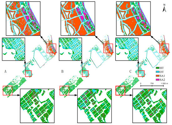
Figure 4.
Comparison of pixel-based classification: (A) decision tree-based classification; (B) support vector machine based classification; and (C) random forest-based classification.
3.1.2. Object-Based Classifications
As with the pixel-based classifications, the major visual difference interpreted between object-based classification maps was also in the north and center of the study area (Figure 5). For the classification of DT and RF, SA1 and SA2 were the dominant species to the northwest and northeast, respectively, whereas the map produced by SVM showed there were not only SA1 and SA2, but also some large patches of HT. In the center of the study area, OT was the dominant community displayed by the object-based classification using the DT algorithm, but in the map produced by the SVM classification, HT was the dominant community, and the map produced by RF classification nearly depicted the same amount of HT and OT. Compared with the field surveying data and original images, we found that half of these islands in the center were covered with HT and the other half were OT, which indicated that the RF based classification was more consistent with real mangrove species. For the south of the study area, HT almost covered every island in the resultant map of SVM and presented regular and complete shape. However, the DT and RF classifications depicted this area as being covered with some large SA2 patches.
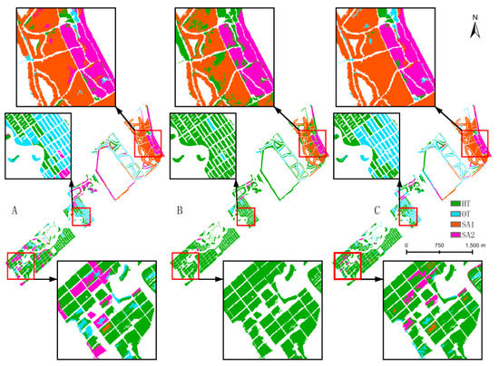
Figure 5.
Comparison of object-based classification: (A) decision tree-based classification; (B) support vector machine-based classification; and (C) random forest-based classification.
3.1.3. Visual Comparison of Pixel-Based and Object-Based Classifications
An overview of all the thematic maps produced by the pixel-based and object-based approaches using the DT, SVM, RF algorithms showed that they had similar depictions of mangrove species, but the local discrepancy was apparent. When the same machine learning algorithm was compared, the representation of SA2, OT/HT, and SA2/OT were major disparities in the DT, SVM and RF classifications, respectively, between the pixel-based and object-based approaches. The classified species patches based on an object-based approach were relatively large in size, and had distinct partition zones and a visually appealing generalized appearance of mangrove species, while the species patches produced by the pixel-based approaches were small and patchier, and presented a noticeable “salt-and-pepper” appearance.
In the Nansha Wetland, SA1, mainly located in the north, is a constructive species and pioneer mangrove species. Due to their generalized appearance and absolute dominance, SA1 was well extracted by all methods, especially in the object-based RF algorithm. The cultivated SA2 was mainly situated in the right side of the north and the center of the study area, which was better represented by the object-based classification than the pixel-based classification. SA2 was well portrayed by the object-based DT and RF algorithms, and was under-represented by all pixel-based image analysis methods. HT was a constructive and dominant community in the south and was planted on regular small islands, which formed an individual Hibiscus tiliaceus community. HT appeared to be better classified by the object-based approach especially in the SVM and RF classifications, but was over-represented from the south to north in the study area by the SVM classification. OT, a combination of eight mangrove species, was over-represented by the pixel-based classifications, and was also under-represented by the object-based classifications.
3.2. Accuracy Assessment and Statistical Comparison
Based on the “hold-out” test data and confusion matrix, the overall classification accuracies of different machine learning algorithms and image analysis approaches were calculated and compared (Table 2). In general, the overall accuracy of the object-based classification outperformed the pixel-based classification except for the SVM algorithm. When using pixel-based methods, the resultant classification using the SVM algorithm had the highest overall classification accuracy (79.63%), followed by the RF (69.44%) and DT (65.74%) classifications. However, when using object-based methods, the resultant classification utilizing the RF algorithm had the highest overall classification accuracy (82.40%), followed by the DT (75.93%) and SVM (73.15%) classifications. It concluded that the SVM algorithm was the most stable classification algorithm for artificial mangrove species, but the object-based RF algorithm produced the best overall classification accuracy.
Table 2.
Confusion matrices and associated classifier accuracies based on test data. SA1 = Sonneratia apetala group 1, SA2 = Sonneratia apetala group 2, HT = Hibiscus tiliaceus, OT = other mangroves. Oa = overall classification accuracy, Pa = producer’s accuracy, Ua = user’s accuracy.
In terms of the user’s accuracy, SA1 was consistent for all classifications and had higher accuracy (>90%), but the other three types had apparent differences. For example, the user’s accuracy for the HT type ranged from 61.64 to 91.43%. In addition, the user’s accuracy of OT was lowest in all mangrove species type on average, especially in pixel-based classifications (about 50%), which indicated that the OT objects had a number of misclassified classifications. Table 2 shows that OT/HT and SA2/OT were the maximum variation types with respect to the user’s accuracy (>25%) between the pixel-based and object-based classifications using the SVM and RF algorithms, respectively, which were consistent with the above visual examination. For the DT classification, the maximum variation species was HT, which exceeded 20%. In terms of the producer’s accuracy, SA1 was still the stable type in all classifications and had higher accuracy, followed by HT, while the other two types varied in different classifications and had lower accuracies, especially for SA2. However, in object-based DT and RF classifications, about two-thirds of HT and OT were still accurately extracted. The producer’s accuracy of HT in the object-based classification using the SVM algorithm was 100%, which further demonstrated the over-fitting phenomenon of HT.
Based on the optimized classification models generated by parameter tuning and “hold-out” validations, we compared different thematic maps using McNemar’s test to examine whether there were statistically significant differences. When comparing the pixel-based with the object-based classifications using the same machine learning algorithm, McNemar’s test showed that the observed difference of DT and SVM models was not statistically significant (p > 0.05) (Table 3), there was even a variation of 10% in the overall classification accuracy between the pixel-based and object-based classifications using the DT algorithm, while it was statistically significant (p = 0.05) between classifications of pixel-based and object-based utilizing the RF algorithm (p = 0.0027).
Table 3.
Statistically significant comparison between pixel-based and object-based classifications when using the same machine learning algorithm.
For the pixel-based classification, statistically significant differences (p = 0.05) between models using the DT and SVM algorithms (p = 0.0027), and SVM and RF algorithms (p = 0.0105) were observed, which was the reason for the outperformance of the SVM algorithm (Table 4). For object-based classification, a statistically significant difference (p = 0.05) was only found between the SVM and RF models (p = 0.0075) with nearly a difference of 10% in overall classification accuracy between them (Table 5).
Table 4.
Statistically significant comparison between three pixel-based machine learning algorithms.
Table 5.
Statistically significant comparison between three object-based machine learning algorithms.
3.3. Comparison of Landscape Pattern
Based on landscape pattern metrics generated by two thematic classification maps, the spatial structure, heterogeneity, fragmentation, and connectivity of the artificial mangroves were compared and analyzed briefly. Before calculating landscape metrics, a filter for both results was performed using the tool “eliminate” in ArcGIS 10.2 (ESRI, Redlands, CA, USA). Polygons less than 10 m2 were merged with the neighboring polygon that has the longest shared border. The comparison of the landscape pattern metrics of the object-based RF classification and pixel-based SVM classification maps at the landscape level and class level are illustrated in Table 6 and Figure 5, respectively.
Table 6.
The comparison of landscape pattern metrics of random forest (RF) object-based and support vector machine (SVM) pixel-based classifications at landscape level.
The total number of mangrove patches (NP) of the study area was 650 for the object-based classification result, while the NP of the pixel-based classification was 6645. The mean patch area (AREA_MN) of mangroves computed from the classifications of RF and SVM were 0.2054 ha/m2 and 0.0201 ha/m2, respectively. The above comparisons of NP and AREA_MN showed that the mangrove species obtained by the object-based classification were far more complete. The largest mangrove species patch (LPI) of object-based classification occupied 8.00% of the total area of mangrove forests, while the LPI of pixel-based classification was just 2.62%. FRAC_AM reflects the shape complexity. Usually, if the shapes are sample perimeters such as squares, FRAC_AM approaches one; if a shape has highly convoluted perimeters, it approaches two. The FRAC_AM of object-based classification was 1.3197 lower than the value of pixel-based classification, indicating that the shape of the object-based map was simpler. CONTAG reflects the aggregation degree of different patch types at a landscape level. Low levels of patch type dispersion (i.e., high proportion of like adjacencies) and low levels of patch type interspersion (i.e., inequitable distribution of pair-wise adjacencies) resulted in a high contagion value approaching 100, and vice versa a value approaching 0. As mangroves were afforested in isolated islands, the CONTAG values of the object-based RF and pixel-based SVM classification were intermediate (52.06 and 50.61, respectively), and mangrove species communities produced by the object-based classification were relatively more aggregate. Shannon’s diversity index (SHDI) is a popular indicator for measuring diversity in community ecology [45]. The SHDI of object-based classification was higher than that of the pixel-based classification.
The area percentage of HT was the largest and its variation the lowest in the pixel-based and object-based classifications, indicating that it was the primary mangrove species in the Nansha Wetland. However, the variations of PLAND for the other three species were apparent, of which OTs were the biggest (Figure 6A). For pixel-based and object-based classifications, the number of patches of the four types differed greatly. The NP of the SA2 in the object-based RF classification was 27 times larger than that of the pixel-based SVM classification, and the NP of the other three mangrove species calculated from the object-based map were about 6 times larger than that of the pixel-based map (Figure 6B). The variation of FRAC_AM for the different mangrove species between pixel-based and object-based classifications ranged from 0.0069–0.1449, and the FRAC_AM of each mangrove species produced by SVM pixel-based classification was bigger than that of object-based classification, except for SA1 (Figure 6C). With respect to aggregation, the AI value of each species produced by object-based classification was greater than that of pixel-based classification, of which the variation of SA1 was the lowest and variation of SA2 was the biggest (Figure 6D).
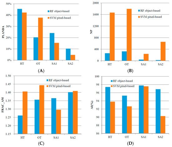
Figure 6.
The comparison of landscape pattern metrics of RF object-based and SVM pixel-based classification at class level: (A) PLAND represents the percentage of landscape; (B) NP represents the number of patches; (C) FRAC_AM represents the area-weighted mean patch fractal dimension; and (D) AI represents the aggregation of patches.
4. Discussion
4.1. The Selection of Pixel-Based and Object-Based Image Analysis Approaches
How to construct a simple, faster, accurate, and repetitive model for extracting mangrove information for a required scale is of concern to geographers, ecologists, and mangrove managers. This study provided streamlined production models for image analysis approaches where the object-based scheme was carried out with the eCognition developer 9.0 software and the pixel-based scheme was implemented with IDL based tools. The results of this study demonstrated that the object-based image analysis approach generally outperformed the pixel-based approach, which is consistent with previous studies [14,20,27,42].
When using McNemar’s test to examine whether there was a statistically significant difference between pixel-based and object-based classifications utilizing the same DT, SVM, and RF algorithms, however, only the RF classification had a statistically significant difference (Table 3). Likewise, based on McNemar’s test, Dingle Robertson and King (2011) [40] and Duro et al. (2012) [20] found no statistically significant difference between the pixel-based and object-based classifications. These studies—including our results—suggested that traditional pixel-based classification could also be used to classify land cover or artificial mangrove species with respect to overall classification accuracy (Table 2).
Usually, when using medium (pixel size 10–30 m) to high (pixel size < 10 m) spatial resolution imagery for vegetation classification in a community level or above, object-based classification can present a more generalized appearance and more contiguous depiction of land cover or target objects, which corresponds more to the actual entity. Whiteside et al. [42] demonstrated this phenomenon and found that the object-based method utilizing the mean spectral value of the segmented object exaggerated the spectral discrimination between spectral mixed species, which could overcome pixel misclassifications in a community-level classification of tropical savanna. In our study, when demarcating spectral mixed mangrove species communities like HT and SA2, this advantage also had an effect (Figure 5). Furthermore, with the increasing computer processing ability, the use of spatial information such as texture and contextual information has become a consensus in image classification for the object-based approach. Pixel-based classification usually only utilizes spectral information. To compensate for the lack of spatial information, we figured out the texture layers and used them for pixel-based supervised classification. Before using texture information, separability values between the four mangrove species calculated by training samples were all below 1.5. While after utilizing the texture layers, these separability values increased to 1.8~2.0. Thus, it was necessary to combine texture with spectral information for both approaches.
However, the object-based classification also has some disadvantages. As segmentation is the basis for object-based classification, some segmented objects contain not only one class of pixels, and larger objects may absorb small rare classes [14,40]. For example, in this study, when we set the scale parameter to the optimal value of 200, there were still some patches of grass or scrub in the mangrove objects. In addition, tuning parameters and the executions of object-based approach were more labor intensive and time consuming in comparison with the pixel-based method.
4.2. The Comparison and Selection of Machine Learning Algorithms
With the development of machine learning algorithms, many new classification models have been produced and provide more choices for classifications of remote sensing images. Every machine learning algorithm has its own suitability and advantages. In this study, RF and SVM performed best in object-based and pixel-based classifications, respectively, with respect to visual examination and overall classification accuracy. Kanniah et al. [19] found that SVM performed worse than MLC for monitoring mangroves. Li et al. [46] declared that SVM outperformed RF for classifying urban tree species. Ghosh and Joshi [47] reported that the RF classification performed worse than the SVM classification for mapping bamboo. Zhang et al. [48], however, found that RF produced higher overall accuracy than SVM for mapping coastal vegetation. Louarn et al. [22] shown that RF slightly outperformed SVM for urban tree species classification. These results showed that when employing different remote sensing images with different classification purposes, machine learning algorithms performed differently.
In general, the DT algorithm was sensitive to segmentation scale variation and robust to the selection of object features, and could perform well at an optimal segmentation scale [21]. For artificial mangrove species discrimination, DT showed an obvious difference between pixel-based and object-based image analysis, and performed poorly in the face of complex mangrove species. Another characteristic of the DT algorithm was that it could export a decision tree plot of a classification, which was very useful for interpreting the logical relationships of classification rule sets [49]. In the study, a decision tree plot helped us to understand how mangrove species were discriminated step by step and which object features with concrete values were used at every tree node.
Likewise, the SVM algorithm was stable with regard to scale and relatively robust in the selection of object features and could perform better with limited training samples than other algorithms [21,50,51]. In this study, the performance of SVM was most stable in different image analysis approaches, but could not only well extract mature and pure mangrove species (SA1), but could also extract partially mixed mangrove species (HT) due to its ability to locate an optimal separating hyperplane for high dimensional features. However, the SVM classification model also suffered from some limitations. The most obvious one was the selection of key parameters of SVM: g (gamma parameter of kernel function) and C (penalty parameter). If g is a small value, it may lead to over-fitting; a large g value may lead to over-smoothing [50]. Due to a lack of heuristics for selecting these SVM parameters, a large number of researchers (including ourselves) have utilized a trial-and-error approach to obtaining the relatively best values [17,19]. In this study, the pixel-based SVM classification was modified in an imageSVM tool [52], which can determine the best fitting values of g and C through an iterative process. However, for the object-based SVM classification, the eCognition developer 9.0 could not optimize these parameters, so we had to test several groups of g and C values and recorded its accuracy after every trial until the relatively highest accuracy was achieved.
As an ensemble classifier, the RF algorithm was robust to the selection of object features and more stable to segmentation scale variation [21,53]. Compared with other state-of-the-art machine learning algorithms, it was more sensitive to training set size and sampling design [54]. On the contrary, RF could greatly benefit from a large and unbiased sample set, which results in high classification accuracy and stable performance [55]. It may be one of the reasons why, in the case of relatively small training samples of artificial mangrove species (111 in this study), the performance of RF also had a conspicuous discrepancy in different image analysis approaches. In addition, the RF classification technique has the ability to handle high dimensional datasets, to measure variable importance, and to keep stable to the parameter configuration [53]. Thus, in the face of partially mixed semi-mangrove species HT, the RF algorithm also extracted it well.
In conclusion, the DT, SVM and RF algorithms could all well map the pure and dominant mangrove species as well as the partly mixed and regular shape mangrove species, but, in the face of complex and easily-confused mangrove species, DT and SVM performed poorly and only the RF algorithm using an object-based image analysis could extract about two-thirds of them. Based on the above results and discussions, for mangrove forest mapping at species level using high spatial resolution images, we recommended the object-based RF classification. In addition, the object-based RF classification may be generalized to classifications of other plants based on high spatial resolution imagery due to the processing chain of them can be easily repeated and applied with nearly no fine tuning [8].
4.3. Feasibility Analysis of Artificial Mangrove Species Classification
Artificial mangroves have long been ignored by researchers. Previous studies have focused on natural mangrove wetlands listed by the Ramsar Convention such as Moreton Bay [13] (Australia), Sungai Pulai, Pulau Kukup, and Tanjung Piai [19] (Malaysia), and Mai Po [56] (Hong Kong). In China, to improve the survival rates and increase the extension of mangroves rapidly, only a few species of native mangroves (Sonneratia caseolaris, Kandelia obovata, Rhizophora stylosa) and exotic species (Sonneratia apetala) have been frequently planted in monoculture for most reforestation projects, which have led to a significant difference between artificial mangrove ecosystems and natural mangrove ecosystems in the community structure and ecological process [4].
For mangrove species classification, there were three challenges, which were as follows [56]: (1) due to the seasonal, tidal, and spectral variability of mangrove species communities, the accurate demarcation of the species community boundaries is very difficult [13,18]; (2) spectral reflectance values of mangroves are often mixed with information of bottom mudflats, water and marginal non-mangrove vegetation [17]; and (3) the spectral differences among mangrove species are subtle [57]. For these reasons, the remote sensing data and methods that have been successfully applied in discriminating terrestrial vegetation species performed poorly in mangrove classification [18]. However, when compared with natural mangrove forests, the community structures of reforested mangroves are relatively simple, most of which are monoculture plantations. Therefore, artificial mangrove classifications using remote sensing techniques are feasible at individual tree species level. Comparing our classification of the highest accuracy with a mangrove thematic map of the same place produced by Qiu et al. [25] by means of manual visual interpretation and quadratic surveys, the area percentage difference of SA and OT between these two classifications were about 6%, and the difference of HT was about 9%, which further demonstrates that artificial mangrove classification is feasible.
Spatial information is essential for artificial mangrove classification. The effectiveness of spatial information (texture in this study) was verified by this study, which could improve the discrimination between mangrove species, especially in pixel-based classification. This was consistent with the conclusions of previous research in mangrove species classifications [28,56]. In general, Landsat TM can only identity vegetation boundaries and mangrove stands, while WorldView-2 can detect all the five scales of mangrove features mentioned above. However, Kamal et al. (2015) [13] showed that in the scale of mangrove zonation, individual tree crowns and species communities, regardless of whether using ALOS AVNIR-2, WorldView-2, or WorldView-2 combined with LIDAR image data, the overall classification accuracies were no more than 70%. When Zhu et al. [28] and Wang et al. [56] used WorldView-2 and WorldView-3 to discriminate the mangroves, respectively, the overall classification accuracies all exceeded 87%. Through comparison, we found that Kamal et al. [13] only used image spectral, distance, and elevation information, but Zhu et al. [28] additionally used shape attributes and the NDVI of objects, and Wang et al. [56] used extra textural and differential spectral features.
In this study, the highest overall classification accuracy was 82.4%, lower than that of Zhu et al. [28] (87.68%) and Wang et al. [56] (90.93%). Their study areas are also located in the Pearl River Estuary and within 45 km of the Nansha Wetland. One of the reasons may be spectral band discrepancies. Like the multispectral image of Pléiades-1, which only has four bands, WorldView-2/3 not only has the same four bands as Pléiades-1 but also has coastal, yellow, red-edge and NIR2 bands. This inference can be supported by the study of Wang and Sousa [57], who distinguished mangrove species with laboratory measurements of hyper-spectral leaf reflectance and asserted that wavebands at 780, 790, 800, 1480, 1530 and 1550 nm were most useful for mangrove species classifications. Likewise, Heenkenda et al. [18] showed that the high spectral resolution was important in obtaining high accuracy for mangrove species identification through a comparison of WorldView-2 with aerial photographs. However, the finding was a limiting factor for purchasing full spectral resolution and high-resolution images (the price of WorldView-2 was 48 U.S.$/km2, and Pléiades-1 was 30 U.S.$/km2, in China, 2017), and now manual visual interpretations and field surveys are the main method for geographers and ecologists to extract mangroves. Therefore, many researchers and managers selected relatively cheap images such as Geoeye-1, Pléiades-1, and GaoFen-1 et al., like Qiu et al. [25]. This is also an important reason as to why we chose Pléiades-1 images as data resources for our research. Compared with a single-data image, bi-temporal Pléiades images can improve the discrimination between tree species, which have been demonstrated by Louarn et al. [22]. In this study, we only used a single-season Pléiades image with all overall classification accuracies below 85%. Therefore, bi-temporal Pléiades images may be an alternative solution in the future. Besides this, we plan to test the new free Sentinel-2 satellite images for mangrove species classifications, which has thirteen appropriate spectral bands ranging from 433 to 2200 nm and provides a consistent time series [8,58]. In conclusion, the appropriate textures and spectrum features can reduce intra-species variability and increase inter-species distinction for mangroves species discriminations.
Geographical location also affects the accuracy of mangrove classification, and the ecological characteristics of a mangrove system in different regions will be obviously discrepant due to variations of water and soil salinity, ocean circulation, tides, topography, soil, climate, and differences in biological factors. Therefore, when the same data and methods are employed in different regions for the remote sensing classification of mangroves, the classification accuracies will be different and the feasibilities may change [18].
5. Conclusions
This study evaluated pixel-based and object-based image analysis approaches with three machine learning algorithms using 0.5-m pan-sharpened images of Pléiades-1 for the purpose of mapping artificial mangrove species in the Nansha Wetland Park, Guangzhou, China. It is the first study dedicated to artificial mangrove species classification using high-resolution remotely sensed imagery.
(1) Both the object-based and pixel-based methods could identity major artificial mangrove species on a community level, but the object-based method had a better performance overall. When conducting the pixel-based image analysis, the SVM algorithm produced the highest overall classification accuracy of 79.63%. When conducting object-based image analysis, the RF algorithm produced the highest overall classification accuracy of 82.40%. The mangrove species patches produced by the object-based approach were relatively large in size, and were more complete and aggregate; while the patches produced by the pixel-based approach were small and patchier, and presented a noticeable “salt-and-pepper” appearance.
(2) When the same machine learning algorithms were compared, a statistically significant difference between the pixel-based and object-based classifications was only found within the RF algorithm. For the pixel-based image analysis, the SVM algorithm produced a classification accuracy that had a statistical difference when compared to the DT and RF algorithms. For object-based image analysis, the statistical difference only existed the between SVM and RF classifications.
(3) When compared to pixel-based approaches with object-based approaches using the same machine learning algorithms, the representation of SA2, OT/HT, and SA2/OT had major discrepancies in the DT, SVM, and RF algorithms, respectively. These discrepant species also had larger omission and commission errors than other species types. Based on visual examination and accuracy reports, the dominant and homogeneous species SA1 could be well classified and the depiction of it was consistent across all classifications, followed by partly mixed and regular shaped mangrove HT, while mixed SA2 and other occasionally presented mangrove species OT could only be identified by major characters with an accuracy of about two-thirds.
The obtained findings make a valuable contribution to the classification methodologies of artificial mangrove species. We recommend repeating this process on larger and more complex study areas with a large area of artificial mangroves restored individually or planted with natural mangrove forests.
Acknowledgments
This study is supported by the National Key Research & Development (R&D) Plan of China (NO. 2016YFB0502304) and the National Science Foundation of China (NO. 41361090). Authors also thank Songjun Xun (School of Geographical Sciences, South China Normal University), who led us when carrying out the mangroves field survey in the Nansha Wetland Park.
Author Contributions
Dezhi Wang, Bo Wan and Xincai Wu conceived and designed the experiments; Dezhi Wang and Bo Wan performed the experiments, analyzed the data and wrote the paper; Yanjun Su, Penghua Qiu and Qinghua Guo contributed to editing and reviewing the manuscript.
Conflicts of Interest
The authors declare no conflict of interest.
References
- Giri, C. Observation and monitoring of mangrove forests using remote sensing: Opportunities and challenges. Remote Sens. 2016, 8, 783. [Google Scholar] [CrossRef]
- Giri, C.; Ochieng, E.; Tieszen, L.L.; Zhu, Z.; Singh, A.; Loveland, T.; Masek, J.; Duke, N. Status and distribution of mangrove forests of the world using earth observation satellite data. Glob. Ecol. Biogeogr. 2011, 20, 154–159. [Google Scholar] [CrossRef]
- Baowen, L.; Qiaomin, Z. Area, distribution and species composition of mangroves in china. Wetl. Sci. 2014, 12, 435–440. (In Chinese) [Google Scholar]
- Chen, L.; Wang, W.; Zhang, Y.; Lin, G. Recent progresses in mangrove conservation, restoration and research in china. J. Plant Ecol. 2009, 2, 45–54. [Google Scholar] [CrossRef]
- Jia, M.M.; Liu, M.Y.; Wang, Z.M.; Mao, D.H.; Ren, C.Y.; Cui, H.S. Evaluating the effectiveness of conservation on mangroves: A remote sensing-based comparison for two adjacent protected areas in shenzhen and hong kong, china. Remote Sens. 2016, 8, 627. [Google Scholar] [CrossRef]
- Kuenzer, C.; Bluemel, A.; Gebhardt, S.; Quoc, V.T.; Dech, S. Remote sensing of mangrove ecosystems: A review. Remote Sens. 2011, 3, 878–928. [Google Scholar] [CrossRef]
- Kamal, M.; Phinn, S.; Johansen, K. Characterizing the spatial structure of mangrove features for optimizing image-based mangrove mapping. Remote Sens. 2014, 6, 984–1006. [Google Scholar] [CrossRef]
- Ng, W.-T.; Rima, P.; Einzmann, K.; Immitzer, M.; Atzberger, C.; Eckert, S. Assessing the potential of sentinel-2 and pléiades data for the detection of Prosopis and Vachellia spp. in Kenya. Remote Sens. 2017, 9, 74. [Google Scholar] [CrossRef]
- Kanniah, K.D.; Wai, N.S.; Shin, A.; Rasib, A.W. Per-pixel and sub-pixel classifications of high-resolution satellite data for mangrove species mapping. Appl. GIS 2007, 3, 1–22. [Google Scholar]
- Wang, L.; Silván-Cárdenas, J.L.; Sousa, W.P. Neural network classification of mangrove species from multi-seasonal ikonos imagery. Photogramm. Eng. Remote Sens. 2008, 74, 921–927. [Google Scholar] [CrossRef]
- Neukermans, G.; Dahdouh-Guebas, F.; Kairo, J.G.; Koedam, N. Mangrove species and stand mapping in gazi bay (Kenya) using quickbird satellite imagery. J. Spat. Sci. 2008, 53, 75–86. [Google Scholar] [CrossRef]
- Wang, L.; Sousa, W.P.; Peng, G.; Biging, G.S. Comparison of ikonos and quickbird images for mapping mangrove species on the caribbean coast of panama. Remote Sens. Environ. 2004, 91, 432–440. [Google Scholar] [CrossRef]
- Kamal, M.; Phinn, S.; Johansen, K. Object-based approach for multi-scale mangrove composition mapping using multi-resolution image datasets. Remote Sens. 2015, 7, 4753–4783. [Google Scholar] [CrossRef]
- Wang, L.; Sousa, W.; Gong, P. Integration of object-based and pixel-based classification for mapping mangroves with ikonos imagery. Int. J. Remote Sens. 2004, 25, 5655–5668. [Google Scholar] [CrossRef]
- Myint, S.W.; Giri, C.P.; Wang, L.; Zhu, Z.L.; Gillette, S.C. Identifying mangrove species and their surrounding land use and land cover classes using an object-oriented approach with a lacunarity spatial measure. GISci. Remote Sens. 2008, 45, 188–208. [Google Scholar] [CrossRef]
- Kamal, M.; Phinn, S. Hyperspectral data for mangrove species mapping: A comparison of pixel-based and object-based approach. Remote Sens. 2011, 3, 2222–2242. [Google Scholar] [CrossRef]
- Heumann, B.W. An object-based classification of mangroves using a hybrid decision tree—Support vector machine approach. Remote Sens. 2011, 3, 2440–2460. [Google Scholar] [CrossRef]
- Heenkenda, M.; Joyce, K.; Maier, S.; Bartolo, R. Mangrove species identification: Comparing worldview-2 with aerial photographs. Remote Sens. 2014, 6, 6064–6088. [Google Scholar] [CrossRef]
- Kanniah, K.; Sheikhi, A.; Cracknell, A.; Goh, H.; Tan, K.; Ho, C.; Rasli, F. Satellite images for monitoring mangrove cover changes in a fast growing economic region in southern peninsular malaysia. Remote Sens. 2015, 7, 14360–14385. [Google Scholar] [CrossRef]
- Duro, D.C.; Franklin, S.E.; Dubé, M.G. A comparison of pixel-based and object-based image analysis with selected machine learning algorithms for the classification of agricultural landscapes using spot-5 HRG imagery. Remote Sens. Environ. 2012, 118, 259–272. [Google Scholar] [CrossRef]
- Li, M.; Ma, L.; Blaschke, T.; Cheng, L.; Tiede, D. A systematic comparison of different object-based classification techniques using high spatial resolution imagery in agricultural environments. Int. J. Appl. Earth Obs. Geoinf. 2016, 49, 87–98. [Google Scholar] [CrossRef]
- Louarn, M.L.; Clergeau, P.; Briche, E.; Deschamps-Cottin, M. “Kill two birds with one stone”: Urban tree species classification using bi-temporal pléiades images to study nesting preferences of an invasive bird. Remote Sens. 2017, 9, 916. [Google Scholar] [CrossRef]
- Li, M.; Lee, S. Mangroves of china: A brief review. For. Ecol. Manag. 1997, 96, 241–259. [Google Scholar] [CrossRef]
- Penghua, Q.; Songjun, X.; Ying, F.; Gengzong, X. A primary study on plant community of wangqingsha semi-constructed wetland in nansha district of guangzhou city. Ecol. Sci. 2011, 30, 43–50. (In Chinese) [Google Scholar]
- Ni, Q.; Songjun, X.; Penghua, Q.; Yan, S.; Anyi, N.; Guangchan, X. Species diversity and spatial distribution pattern of mangrove in nansha wetland park. Ecol. Environ. Sci. 2017, 26, 27–35. (In Chinese) [Google Scholar]
- Sarp, G. Spectral and spatial quality analysis of pan-sharpening algorithms: A case study in istanbul. Eur. J. Remote Sens. 2014, 47, 19–28. [Google Scholar] [CrossRef]
- Vo, Q.T.; Oppelt, N.; Leinenkugel, P.; Kuenzer, C. Remote sensing in mapping mangrove ecosystems—An object-based approach. Remote Sens. 2013, 5, 183–201. [Google Scholar] [CrossRef]
- Zhu, Y.; Liu, K.; Liu, L.; Wang, S.; Liu, H. Retrieval of mangrove aboveground biomass at the individual species level with worldview-2 images. Remote Sens. 2015, 7, 12192–12214. [Google Scholar] [CrossRef]
- Costa, H.; Foody, G.M.; Boyd, D.S. Using mixed objects in the training of object-based image classifications. Remote Sens. Environ. 2017, 190, 188–197. [Google Scholar] [CrossRef]
- McFeeters, S.K. The use of the normalized difference water index (NDWI) in the delineation of open water features. Int. J. Remote Sens. 1996, 17, 1425–1432. [Google Scholar] [CrossRef]
- Van Coillie, F.M.; Verbeke, L.P.; De Wulf, R.R. Feature selection by genetic algorithms in object-based classification of ikonos imagery for forest mapping in flanders, belgium. Remote Sens. Environ. 2007, 110, 476–487. [Google Scholar] [CrossRef]
- Vaudour, E.; Carey, V.A.; Gilliot, J.M. Digital zoning of south african viticultural terroirs using bootstrapped decision trees on morphometric data and multitemporal spot images. Remote Sens. Environ. 2010, 114, 2940–2950. [Google Scholar] [CrossRef]
- Van der Linden, S.; Rabe, A.; Held, M.; Jakimow, B.; Leitão, P.; Okujeni, A.; Schwieder, M.; Suess, S.; Hostert, P. The enmap-box—A toolbox and application programming interface for enmap data processing. Remote Sens. 2015, 7, 11249–11266. [Google Scholar] [CrossRef]
- Breiman, L. Random forests. Mach. Learn. 2001, 45, 5–32. [Google Scholar] [CrossRef]
- Immitzer, M.; Atzberger, C.; Koukal, T. Tree species classification with random forest using very high spatial resolution 8-band worldview-2 satellite data. Remote Sens. 2012, 4, 2661–2693. [Google Scholar] [CrossRef]
- Su, Y.; Ma, Q.; Guo, Q. Fine-resolution forest tree height estimation across the sierra nevada through the integration of spaceborne lidar, airborne lidar, and optical imagery. Int. J. Digit. Earth 2017, 10, 307–323. [Google Scholar] [CrossRef]
- Rodriguez-Galiano, V.F.; Ghimire, B.; Rogan, J.; Chica-Olmo, M.; Rigol-Sanchez, J.P. An assessment of the effectiveness of a random forest classifier for land-cover classification. ISPRS J. Photogramm. Remote Sens. 2012, 67, 93–104. [Google Scholar] [CrossRef]
- Stehman, S.V. Thematic map accuracy assessment from the perspective of finite population sampling. Int. J. Remote Sens. 1995, 16, 589–593. [Google Scholar] [CrossRef]
- Foody, G.M. Thematic map comparison: Evaluating the statistical significance of differences in classification accuracy. Photogramm. Eng. Remote Sens. 2004, 70, 627–633. [Google Scholar] [CrossRef]
- Robertson, L.D.; King, D.J. Comparison of pixel- and object-based classification in land cover change mapping. Int. J. Remote Sens. 2011, 32, 1505–1529. [Google Scholar] [CrossRef]
- Foody, G.M. Sample size determination for image classification accuracy assessment and comparison. Int. J. Remote Sens. 2009, 30, 5273–5291. [Google Scholar] [CrossRef]
- Whiteside, T.G.; Boggs, G.S.; Maier, S.W. Comparing object-based and pixel-based classifications for mapping savannas. Int. J. Appl. Earth Obs. Geoinf. 2011, 13, 884–893. [Google Scholar] [CrossRef]
- Vaz, E. Managing urban coastal areas through landscape metrics: An assessment of mumbai’s mangrove system. Ocean Coast. Manag. 2014, 98, 27–37. [Google Scholar] [CrossRef]
- Li, H.; Wu, J. Use and misuse of landscape indices. Landsc. Ecol. 2004, 19, 389–399. [Google Scholar] [CrossRef]
- Wang, D.; Qiu, P.; Fang, Y. Scale effect of li-xiang railway construction impact on landscape pattern and its ecological risk. Chin. J. Appl. Ecol. 2015, 26, 2493–2503. [Google Scholar]
- Li, D.; Ke, Y.H.; Gong, H.L.; Li, X.J. Object-based urban tree species classification using bi-temporal worldview-2 and worldview-3 images. Remote Sens. 2015, 7, 16917–16937. [Google Scholar] [CrossRef]
- Ghosh, A.; Joshi, P.K. A comparison of selected classification algorithms for mapping bamboo patches in lower gangetic plains using very high resolution worldview 2 imagery. Int. J. Appl. Earth Obs. Geoinf. 2014, 26, 298–311. [Google Scholar] [CrossRef]
- Zhang, C.Y.; Xie, Z.X. Data fusion and classifier ensemble techniques for vegetation mapping in the coastal everglades. Geocarto Int. 2014, 29, 228–243. [Google Scholar] [CrossRef]
- Mallinis, G.; Koutsias, N.; Tsakiri-Strati, M.; Karteris, M. Object-based classification using quickbird imagery for delineating forest vegetation polygons in a mediterranean test site. ISPRS J. Photogramm. Remote Sens. 2008, 63, 237–250. [Google Scholar] [CrossRef]
- Mountrakis, G.; Im, J.; Ogole, C. Support vector machines in remote sensing: A review. ISPRS J. Photogramm. Remote Sens. 2011, 66, 247–259. [Google Scholar] [CrossRef]
- Silva, J.; Bacao, F.; Caetano, M. Specific land cover class mapping by semi-supervised weighted support vector machines. Remote Sens. 2017, 9, 181. [Google Scholar] [CrossRef]
- Okujeni, A.; van der Linden, S.; Suess, S.; Hostert, P. Ensemble learning from synthetically mixed training data for quantifying urban land cover with support vector regression. IEEE J. Sel. Top. Appl. Earth Obs. Remote Sens. 2017, 10, 1640–1650. [Google Scholar] [CrossRef]
- Pelletier, C.; Valero, S.; Inglada, J.; Champion, N.; Dedieu, G. Assessing the robustness of random forests to map land cover with high resolution satellite image time series over large areas. Int. J. Remote Sens. 2016, 187, 156–168. [Google Scholar] [CrossRef]
- Belgiu, M.; Dragut, L. Random forest in remote sensing: A review of applications and future directions. ISPRS J. Photogramm. Remote Sens. 2016, 114, 24–31. [Google Scholar] [CrossRef]
- Millard, K.; Richardson, M. On the importance of training data sample selection in random forest image classification: A case study in peatland ecosystem mapping. Remote Sens. 2015, 7, 8489–8515. [Google Scholar] [CrossRef]
- Wang, T.; Zhang, H.; Lin, H.; Fang, C. Textural–spectral feature-based species classification of mangroves in mai po nature reserve from worldview-3 imagery. Remote Sens. 2016, 8, 24. [Google Scholar] [CrossRef]
- Wang, L.; Sousa, W.P. Distinguishing mangrove species with laboratory measurements of hyperspectral leaf reflectance. Int. J. Remote Sens. 2009, 30, 1267–1281. [Google Scholar] [CrossRef]
- Barton, I.; Király, G.; Czimber, K.; Hollaus, M.; Pfeifer, N. Treefall gap mapping using sentinel-2 images. Forests 2017, 8, 426. [Google Scholar] [CrossRef]


© 2018 by the authors. Licensee MDPI, Basel, Switzerland. This article is an open access article distributed under the terms and conditions of the Creative Commons Attribution (CC BY) license (http://creativecommons.org/licenses/by/4.0/).