Abstract
Coastal water-quality is both a primary driver and also a consequence of coastal ecosystem health. Turbidity, a measure of dissolved and particulate water-quality matter, is a proxy for water quality, and varies on daily to interannual periods. Turbidity is influenced by a variety of factors, including algal particles, colored dissolved organic matter, and suspended sediments. Identifying which factors drive trends and extreme events in turbidity in an estuary helps environmental managers and decision makers plan for and mitigate against water-quality issues. Efforts to do so on large spatial scales have been hampered due to limitations of turbidity data, including coarse and irregular temporal resolution and poor spatial coverage. We addressed these issues by deriving a proxy for turbidity using ocean color satellite products for 11 Gulf of Mexico estuaries from 2000 to 2014 on weekly, monthly, seasonal, and annual time-steps. Drivers were identified using Akaike’s Information Criterion and multiple regressions to model turbidity against precipitation, wind speed, U and V wind vectors, river discharge, water level, and El Nino Southern Oscillation and North Atlantic Oscillation climate indices. Turbidity variability was best explained by wind speed across estuaries for both time-series and extreme turbidity events, although more dynamic patterns were found between estuaries over various time steps.
1. Introduction
The quality of estuarine and other coastal waters is a complex function of hydrological, meteorological, oceanographic, and human drivers [1,2,3,4]. The relative influence of these processes affects water-quality trends, variability, and the occurrence of extreme water-quality events. Identifying the primary drivers of such events can be useful for management and mitigation purposes. For example, a state of emergency was declared in two Florida counties in 2016 as a result of thick algal mats growing along highly populated coastal waterways in the St. Lucie and Caloosahatchee estuaries, causing massive fish kills [5]. This emergency was caused by the release of nutrient-rich waters from Lake Okeechobee. A commentary published by Michalak [5] called for targeted research to determine which environmental conditions, and in what combination, increase the likelihood of extreme water-quality issues.
Turbidity is an index of water quality used by the U.S. Environmental Protection Agency (EPA) that measures light transparency in aquatic environments. Turbidity may be modulated by changes in the concentration of colored dissolved organic matter and suspended particulates including sediment and phytoplankton, which are affected by changes in hydrological, meteorological, and oceanographic phenomena [2,6,7].
According to the 2012 EPA National Coastal Condition Report (NCCR), the overall rating of Gulf coast waters was 2.4 out of 5, or “fair” [8]. Approximately 10% of the coastal waters were rated “poor”, and 53% were rated “fair” for water quality index. More specifically, water clarity was rated poor for 21% of the area. In Tampa Bay, Florida, water quality—measured by turbidity and average chlorophyll concentration—has improved since the 1970s [4,9]. This is primarily attributed to the upgrade of wastewater treatment plants to tertiary level starting in 1979. This reduced point-source pollution to the bay. Greening et al. [10] found that the point and nonpoint sources of nitrogen to Tampa Bay were 60.3% and 23.9%, respectively, of the total nitrogen loadings in the 1970s. By the 2000s, the total pollution was reduced by about half, but relative contributions were inverted, with point sources contributing about 19.5% and nonpoint 57.4% to nitrogen discharges into the bay. Comparing these results to other Gulf of Mexico (GoM) estuaries is difficult given the lack of robust water quality monitoring programs, but the NCCR indicate that, since 2000 GoM coastal water quality indices and their component indicators show no significant linear trend over time in areas rated poor [8]. In order to continue improving water-quality management in these estuaries, we must better understand the drivers of nonpoint-source water-quality degradation, and constrain their relative effects on long-term trends as well as extreme events in the bays. Doing so requires long time-series of water quality and potential environmental drivers with sufficient spatial and temporal resolution to characterize variability and enable management actions.
Precipitation within a drainage basin influences water quality through increased nutrient and sediment discharge into rivers [7,11,12]. Wind also influences water quality through sediment resuspension in coastal areas [13,14,15]. Schoen et al. [16] modeled circulation in an estuarine lake and found that circulation patterns were highly influenced by diurnal wind speed and direction variability, driving significant intermittent mixing. Dixon et al. [17] studied seasonal colored dissolved organic matter (CDOM) sources within a North Carolina estuary, and found that water quality was controlled by wind speed, wind direction, and river discharge.
River discharge increases nutrient and sediment loads to coastal waters, thereby increasing turbidity with suspended sediments, CDOM, and phytoplankton blooms [18,19]. Dorado et al. [20] evaluated the effects of freshwater inflow on phytoplankton in Galveston Bay, Texas, and found that a combination of nutrient loading and hydraulic displacement drove phytoplankton biomass and community composition throughout the bay.
In addition to wind and freshwater-inflow variability, other forces drive estuarine water quality by influencing circulation, sediment suspension, and coastal erosion. Over hourly to daily periods, tidal circulation can impact estuarine phytoplankton and suspended sediment concentrations [21]. Over longer periods, the sea-level cycle of the Gulf coast has changed such that more extreme (i.e., lower in winter and higher in summer) water levels are now observed [22]. While long-term water level is not typically investigated for effects on water quality, we include it here to account for apparent changes in this fundamental element of estuarine composition.
While each of these environmental variables has been shown or hypothesized to influence local water quality parameters, broader climatic variability may explain long-term patterns in regional water quality. Scarsbrook et al. [23] studied the effects of El Niño-Southern Oscillation (ENSO) patterns on New Zealand riverine water quality and found significant relationships between them, even after accounting for river flow variability. Their results suggested that ENSO significantly impacted water quality, independent of indirect effects through known precipitation variability caused by ENSO patterns. Schmidt et al. [24] evaluated the effects of ENSO patterns on precipitation and river discharge throughout Florida’s watersheds, and found a complex pattern of spatially variable, seasonal relationships, including statistically significant relationships between extreme ENSO events and winter precipitation and river discharge patterns in the Tampa Bay area.
The North Atlantic Oscillation (NAO) also drives seasonal wind and precipitation patterns in the Southeast [25]. The NAO is defined as a meridional alternation of atmospheric mass between the subtropical and arctic North Atlantic. NAO phases may vary from one year to the next, and are greatest in amplitude during November to April [26]. Kenyon and Hegerl [27] quantified the impact of the NAO on global precipitation extremes and found that, while more closely connected with European precipitation, statistically significant responses were found in some North American precipitation stations, including those along the GoM coast.
Turbidity data collected in-situ from individual sampling stations may reflect localized phenomena. To evaluate bay-wide turbidity patterns, we need time series of synoptic turbidity observations. For large estuaries spanning several tens of kilometers in length and width, traditional ocean color satellite imagery can improve spatial and temporal sampling of water quality by providing data for the entire estuary in a single observation, often at near daily intervals [28]. Chen et al. [21] employed in-situ sensors and satellite data to determine the mechanisms responsible for observed variability in phytoplankton and sediment in Tampa Bay over a two-month period. They identified three strong wind events, which generated critical bottom shear stress and suspended bottom sediments that were observed in concurrent Moderate Resolution Imaging Spectroradiometer (MODIS) imagery. They concluded that collecting a single monthly grid of samples with one water sample per station per month can lead to variability of −50% to 200% of particular samples relative to the monthly mean of chlorophyll or sediment. Fernandez-Novoa et al. [19] used imagery from MODIS to study turbidity plumes from the Ebro River over the period 2003–2011. There was sufficient coverage to isolate specific environmental conditions coinciding with satellite overpasses, including specific river discharge conditions and wind patterns. With this dataset they were able to identify the direction and extent of river plume events into the Mediterranean, and concluded that wind direction was the dominant driver of turbidity magnitude.
Eleven GoM estuaries from Texas to Florida were selected for this study to provide a synoptic assessment of water-quality drivers throughout the U.S. Gulf coast. These estuaries were chosen, in part, because the surface area of each (Table 1) is large enough to accommodate the 250 m spatial resolution of MODIS imagery. Additionally, all of these estuaries are adjacent to large population centers, and therefore their health and management may impact more stakeholders than isolated estuaries.

Table 1.
National Estuary Programs (NEP) studied here and relevant characteristics.
The objective of this study was to determine the meteorological, oceanographic, and atmospheric drivers of water quality time-series and extreme events in 11 GoM estuaries between 2000 and 2014 using a satellite-derived proxy for turbidity binned to weekly, monthly, seasonal and annual time steps. The estuaries studied include: Aransas Bay, Barataria Bay, Charlotte Harbor, Corpus Christi Bay, Galveston Bay, Matagorda Bay, Mobile Bay, San Antonio Bay, Sarasota Bay, Tampa Bay, and Terrebonne Bay. The explanatory variables investigated include: Precipitation, wind speed, U and V wind vectors, river discharge, water level, and ENSO and NAO climate indices.
Study Areas
Each of the 11 estuaries studied here is a designated member of the National Estuary Program (Figure 1). The NEP is an EPA program created to protect and restore the water quality and ecological integrity of national estuaries.
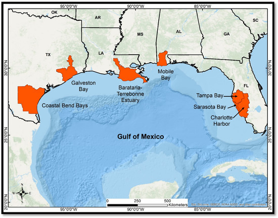
Figure 1.
Environmental Protection Agency National Estuary Programs of the Gulf of Mexico studied here.
Charlotte Harbor (CH), Florida, is a water body of 805 km2 and 2.4 m deep on average that receives water from a watershed extending over 12,000 km2 of southwestern Florida [29]. Sarasota Bay (SB), Florida, lies between Charlotte Harbor to the south and Tampa Bay to the north. It drains the smallest watershed (1100 km2) of those evaluated in this study, and covers the smallest surface water area at just over 100 km2 (https://sarasotabay.org/). Tampa Bay (TB), Florida covers over 1000 km2 with an average depth of 3.4 m, and drains a watershed of over 6500 km2 [30]. Six counties and the cities of Tampa, Clearwater, and Saint Petersburg intersect the watershed, making it the second largest metropolitan area in Florida.
Mobile Bay (MB) is located along the northern Gulf Coast in the state of Alabama. With an inflow of 1755 m3/s, it receives 20% of the freshwater supply in the US and is the fourth largest estuary in the country draining a watershed of 113,084 km2 [31].
The Barataria (BTB) and Terrebonne (TBB) estuaries are distinct bodies of water with separate watersheds, but are managed as a single NEP. They are located between the Mississippi and Atchafalaya Rivers in southern Louisiana. Freshwater input was effectively cut off by the flood protection levees erected along the Mississippi River such that rainwater constitutes the primary source of it. These bays are bounded to the south by barrier islands that are expected to decline in size from 7.3 km2 to 1.6 km2 by 2045 due to erosion, resulting in greater tidal mixing (https://www.lacoast.gov).
Galveston Bay (GB), Texas, is the seventh largest estuary in the country with over 1500 km2 of surface water and the fourth most populous metropolitan area in the country. The estuary has experienced substantial environmental degradation, losing over 95% of submerged vegetation from the 1950s to 1970s due in part to poor water clarity caused by increased erosion [32].
The Coastal Bend Bays NEP includes Aransas Bay (ARB) and Corpus Christi Bay (CCB). We also included the adjacent bodies of San Antonio (SAB), and Matagorda (MGB) Bays to these analyses. These four water bodies combined cover over 1300 km2 and drain the second largest watershed of those studied here at 32,580 km2 (Table 1).
2. Materials and Methods
All preprocessing of independent variables, and statistical analyses were conducted using MatlabTM and the Fathom toolbox.
2.1. Turbidity Proxy
We used satellite data from the NASA Moderate Resolution Imaging Spectroradiometer (MODIS) sensor flown on the Terra satellite to derive a proxy for turbidity. MODIS Terra has provided a time-series of remote sensing observations at relatively high temporal resolution (near-weekly or better at the latitudes of Gulf estuaries) and high spatial resolution (250 m to 1 km) since 2000. Specifically, we generated time-series of water quality indices using remote-sensing reflectance from MODIS Terra Band 1 (645 nm band center with a spatial resolution of 250-m; band range is 620–670 nm) as a proxy. The basic assumption is that sediments suspended near the water surface provide a signal in this red band. In general, we assumed that MODIS Band 1 observations have minimal contributions from light reflected from the sea bottom in estuarine waters deeper than about 2.8 m due to the strong absorption of red light by water [21]. This approach has been used several times in the past, with mixed success, in different estuaries and coastal waters around the world [6,13,14,21,33,34,35,36,37,38,39]. Other bio-optical algorithms that utilize blue, green, or yellow bands to estimate parameters such as chlorophyll-a concentration are usually contaminated by reflectance from the ocean bottom in shallow areas and don’t provide accurate estimates.
We derived remote sensing reflectance at 645 nm (Rrs645) starting from MODIS Terra Level-1A files. Rrs645 represents the normalized water-leaving radiance [40] at 645 nm divided by the extraterrestrial solar irradiance at 645 nm. MODIS images were downloaded from the NASA Goddard Space Flight Center Ocean Color data portal (https://oceancolor.gsfc.nasa.gov/). Images were processed using the SeaWiFS Data Analysis System (SeaDAS) software package, version 7.1. Processing to Level-2 used the near infrared/short-wave infrared (NIR/SWIR) switching atmospheric correction approach of Wang and Shi [41]. All data were mapped to an equidistant cylindrical projection with a nominal pixel size of 262 m. Using the SeaDAS l2gen module, masks were applied for clouds, stray light, and sun glint. A custom filter file was used to mask stray light using a 1 × 1 pixel filter, as opposed to the default 3 × 3 pixel filter. The cloud mask was applied using data at 2130 nm with a threshold of 0.018 [36]. Individual scenes with high cloud cover (>85%) and sun glint contamination, as indicated in the data flags, were removed. The total number of images used per estuary varied between estuaries, and ranged from 3424 to 3958 images. To minimize the effects of negative Rrs645 retrievals, the median value of all negative Rrs645 values was calculated and applied as a bias to each MODIS scene [36]. Values of this bias ranged from −0.002 sr−1 to zero, and are likely caused by aerosol overestimation. All remaining negative pixels were excluded from further analyses.
2.2. Meteorological Data
Daily precipitation, wind speed, and wind direction data were downloaded from the NOAA National Centers for Environmental Information (formerly the National Climate Data Center; https://www.ncei.noaa.gov/) for the stations listed in Table 2. Stations were selected from all available stations adjacent to each estuary that contained data for each variable covering the 2000–2014 time period. Precipitation data were binned to weekly, monthly, seasonal, and annual time steps by summing the data for each interval. We chose to represent precipitation cumulatively for two reasons: occasional downpours characteristic of Gulf coast winter frontal systems and summer convective storms may substantially influence runoff and erosion, but their extreme nature may be muted by averaging with surrounding days or weeks of little or no rain; and consistent rain over days or weeks may synergistically impact drainage by reaching a soil saturation point beyond which surface runoff may increase. Unfortunately, precipitation data from all stations adjacent to the Barataria-Terrebonne NEP were missing more than 25% of daily observations for this time period, and were therefore excluded from analyses.
Table 2.
Station locations used for meteorological, river discharge, and water level data for each estuary.
Wind data were binned to the same time steps as precipitation, but used an average for each time step. Coincident wind speed and direction observations were converted to U (east-west) and V (north-south) component vectors prior to temporal binning.
2.3. River Discharge Data
Daily measurements of river discharge were downloaded from the United States Geological Survey website (https://maps.waterdata.usgs.gov/mapper/index.html?state) for every monitored river system that entered into each estuary. Rivers that were regulated with known dams or bypasses, such as Hillsborough River in Tampa Bay, were excluded to eliminate potentially anomalous anthropogenic influence. That is, management of Hillsborough River discharge is likely to primarily affect Hillsborough Bay—a subset of Tampa Bay—and therefore not be resolved by the bay-wide turbidity proxy. When data was available for multiple rivers that discharged into the same estuary, each dataset of daily discharge measurements was compared with daily Rrs645 measurements to determine if substantial gaps in discharge data existed (i.e., days for which Rrs645 observations were made, but not for discharge data). If a discharge dataset was missing more than 25% of daily observations (i.e., data gaps), that discharge dataset was considered too sparse for evaluation and excluded from further analyses. If, however, multiple rivers for a given estuary were found to be sufficient, their data were combined into one discharge dataset for that estuary by summing daily measurements, and then binning the data to the weekly, monthly, seasonal and annual time steps by average. Table 2 lists the rivers used for each estuary. For both Barataria and Terrebonne Bays, water level data from the Gulf Intracoastal Waterway (GIWW) station at Houma, Louisiana, was used.
2.4. Water Level Data
Hourly water-level data were downloaded from the NOAA website (tidesandcurrents.noaa.gov) for all stations monitored during the time period and located within the estuaries (MLLW datum; Table 2). Verified water-level data was missing more than 25% of daily observations for the study period within the Sarasota Bay, Corpus Christi Bay, Matagorda Bay, or San Antonio Bay estuaries. Data from Tampa Bay was assumed to be a sufficient proxy for Sarasota Bay, as was data from Aransas Bay for the three adjacent Coastal Bend Bays. Datasets were binned to weekly, monthly, seasonal, and annual time steps by average.
2.5. NAO Data
Daily NAO index data was downloaded from NOAA (ftp://ftp.cpc.ncep.noaa.gov/cwlinks/norm.daily.nao.index.b500101.current.ascii) and binned to the same time steps.
2.6. ENSO Data
Monthly Niño-3.4 index data was downloaded from NOAA (http://www.cpc.ncep.noaa.gov/products/analysis_monitoring/ensostuff/detrend.nino34.ascii.txt) and binned to seasonal and annual time steps. As weekly data was not available, the ENSO variable was excluded from weekly analyses.
2.7. Preprocessing
Observations from each dataset for each time step were first matched to the Rrs645 dataset by identifying coinciding observations. This allowed for a direct comparison of datasets to identify gaps. If any independent variable for a given estuary matched fewer than 75% of Rrs645 observations, that variable was eliminated from further analyses. A linear trend was then fit to each dataset and removed (detrended). Next, climatologies for each time step were computed for each detrended dataset from the 15-year period of available data. Typically, climatologies are computed using 30-year time periods, but many of the datasets used for this work, including Rrs645, did not have 30 years of available data. We chose to restrict climatologies to the 15-year period evaluated here for consistency between datasets. Anomalies were computed by subtracting the climatology values from the coinciding time-series observation. Extreme events were identified as those Rrs645 observations within the 90th and 95th percentiles of each estuary’s dataset. The time-series anomalies, and 90th and 95th percentile extreme-event anomalies (hereafter “XE90” and “XE95”) were then used for statistical analyses.
2.8. Statistical Analyses
Redundancy Analyses with Akaike’s Information Criterion (RDA AIC) were used first to identify the independent variables that explained the most variation in the dependent variable. The f_rdaAIC MatlabTM function from the Fathom toolbox standardized all input independent variables and determined the ‘best’ independent variables through constrained ordination. This assessed how much of the variation in one set of variables explained variation in another set, while accounting for multicollinearity between independent variables [42]. Akaike [43] proposed an information criterion to quantify the amount of information and statistically determine the number of parameters for an equation that represents a group of experimental data. The equation with the minimum AIC is considered the best representation of the experimental data [44]. A null model is created by assigning a value below which the best equation’s AIC value must be in order to be considered viable to explain variation in the dependent variable. If no equation explains more variation than a null model, no independent variable is selected.
For any variable(s) identified as ‘best’ for a given estuary, correlation coefficients were computed with all other variables using the “corrcoef” Matlab function. If any correlations with ‘best’ variables exceeded ±0.7, the correlated variables were recorded for consideration.
Multiple regressions were run on the variable(s) identified as ‘best’ by the RDA AIC using the f_mregress function. One thousand iterations were run for each regression to compute permutation-based p values because some of the data were not normally distributed. Adjusted-R2 coefficients (R2adj) were recorded, as opposed to R2 coefficients, because the former accounts for the number of predictors and sample size. Figure 2 summarizes the data on which statistical analyses were performed.
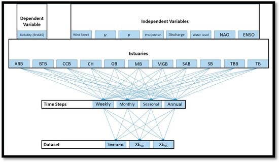
Figure 2.
Summary of the variables, estuaries, time steps and datasets used for statistical analyses.
3. Results
To identify the drivers of turbidity across the coastal GoM, we evaluated the results of statistical analyses by estuary, time step, and time series or extreme event dataset. The variable(s) identified as statistically significant drivers of time-series, XE90 and XE95 turbidity for each estuary over all four time steps are indicated in Table 3 by the number of time steps (0–4) in which they were found to be significant. Additionally, the number of estuaries (0–11) for which each variable was identified as a statistically significant driver is summarized in the Table 4 by time step. The results of each individual iteration, including R2adj, p, sample size, correlations, etc., are reported in Supplemental Materials.
Table 3.
The number of time steps (0–4) for which each variable was identified as a significant driver (R2adj > 0.2, p < 0.05) of turbidity time-series, 90th percentile events (in parentheses), and 95th percentile events [in brackets] for each estuary. Positive results shaded grey.
Table 4.
The number of estuaries (0–11) for which each variable was identified as a significant driver (R2adj > 0.2, p < 0.05) of turbidity time-series, 90th percentile events (in parentheses), and 95th percentile events [in brackets] for each time step. Positive results shaded grey.
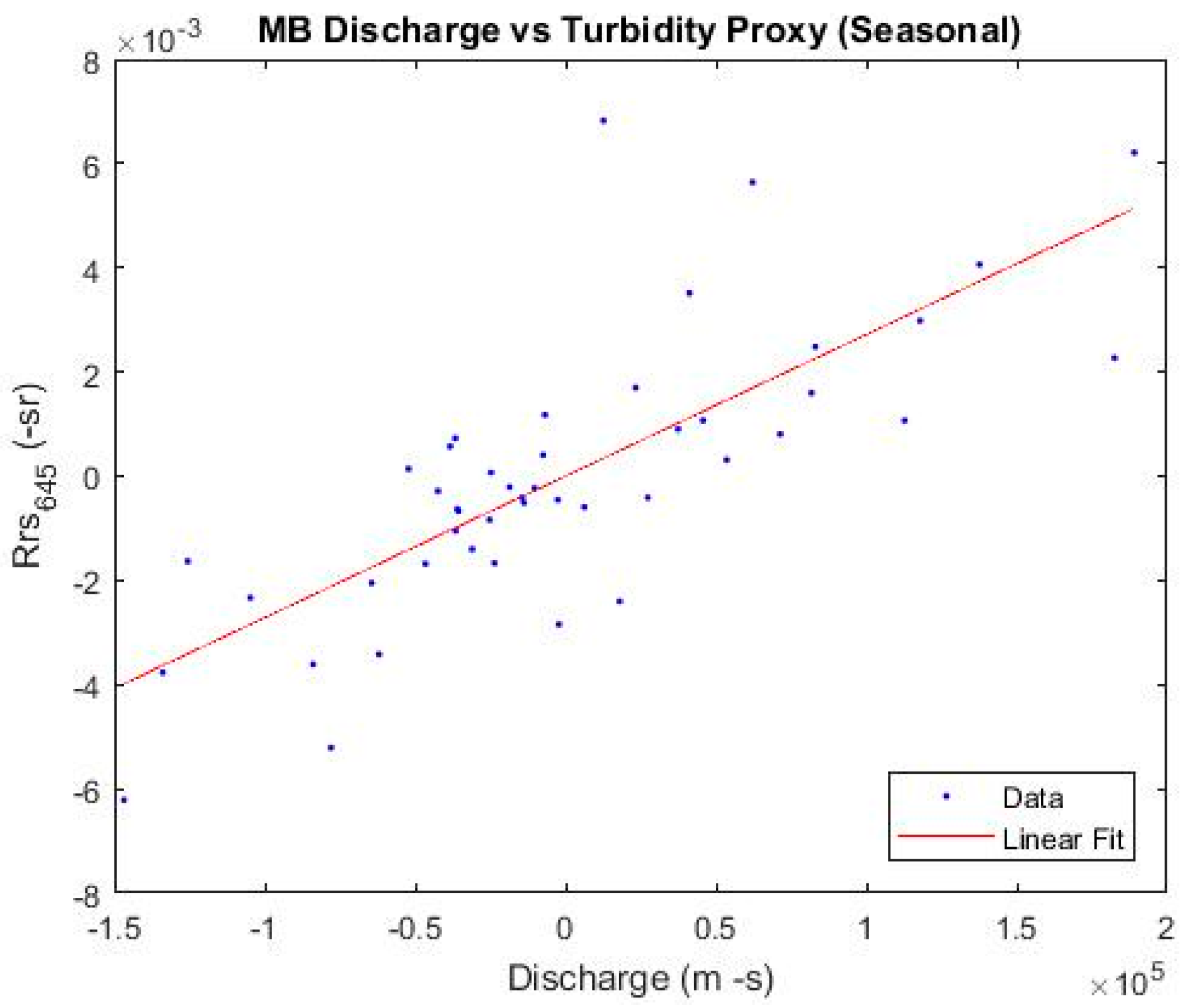
Analyses of time series data identified statistically significant relationships (p < 0.05) between turbidity and at least one independent variable for all time steps (i.e., weekly, monthly, seasonal, and annual) in all estuaries, with the exception of nine iterations. That is, no variables were identified as “best” by the AIC step in four runs, and only five runs identified at least one “best” variable, but the resulting model could not explain turbidity variation significantly. Excluding those results, the variables most often found to explain turbidity variation were wind speed (25 iterations) and discharge (15 iterations). If we exclude those statistically significant relationships that found R2adj values under 0.2, the variables found to most frequently explain turbidity variation were discharge (9 times; Figure 3) and wind speed (8 times; Table 3). Discharge data was found to contain too many gaps to be sufficient for weekly or monthly analyses in Galveston Bay. In addition, water level was excluded from Terrebonne Bay weekly and monthly analyses for the same reason.
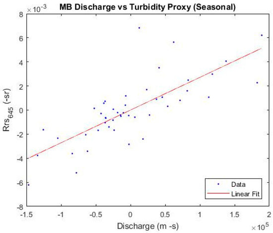
Figure 3.
Plot of Mobile Bay seasonal time-series discharge vs. turbidity proxy anomalies (R2adj = 0.570, p = 0.001, n = 46).
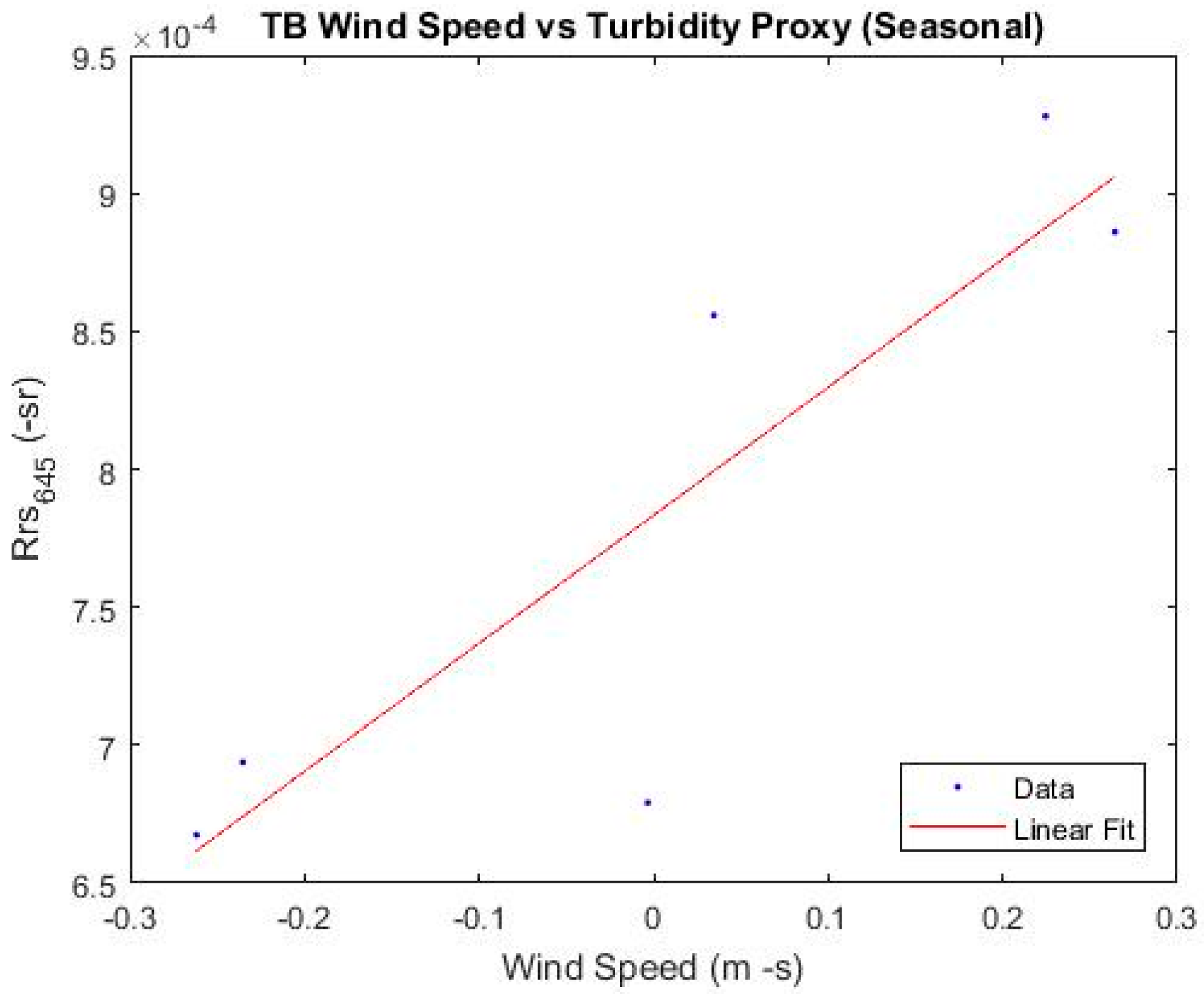
Analyses of 90th percentile extreme events (XE90) found statistically significant relationships between turbidity and at least one independent variable in 20 of the 44 analyses. None of the annual analyses identified a “best” variable, probably due to low sample sizes. For all analyses that identified a significant variable, wind speed (7 times; Figure 4) was identified the most, followed by ENSO (6 times), and discharge (3 times). Excluding significant relationships with R2adj values under 0.2, the variables found to most frequently explain turbidity variation were ENSO (6 times), and wind speed (4 times; Table 3). Discharge and water level were excluded from Galveston Bay and Terrebonne Bay, respectively, due to insufficient data.

Figure 4.
Plot of Tampa Bay seasonal XE90 wind speed vs. turbidity proxy anomalies (R2adj = 0.707, p = 0.001, n = 6).
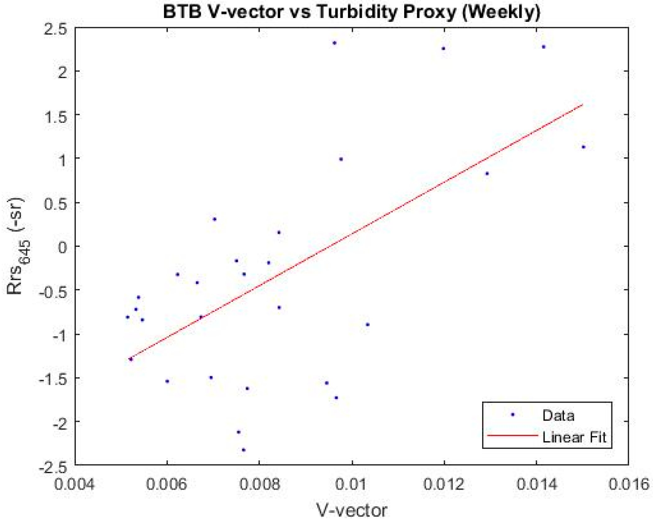
Analyses of 95th percentile extreme events (XE95) found statistically significant relationships between turbidity and at least one independent variable in 7 of the 44 runs. None of the seasonal or annual runs identified a “best” variable, probably due to low sample sizes. For all runs that identified a significant variable, the V vector (3 times), and U vector (2 times) were identified most. Excluding significant relationships with R2adj values under 0.2, the variable found to most frequently explain turbidity variation was the V vector (2 times; Table 3; Figure 5). Discharge and water level were excluded from Galveston Bay and Terrebonne Bay, respectively, due to insufficient data.
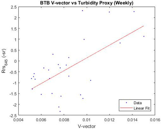
Figure 5.
Plot of Barataria Bay weekly XE95 V-vector vs turbidity proxy anomalies (R2adj = 0.355, p = 0.001, n = 28).
4. Discussion
We will refer to variables that were identified as statistically significantly (p < 0.05) correlated to the Rrs645 turbidity proxy with R2adj values greater than 0.2 as “significant drivers” of turbidity. Because RDA AIC and multiple regression analyses may identify more than one variable per iteration, we will discuss the results by noting both the number of estuaries for which an independent variable was identified as a driver, and the number of times a variable was identified as a driver.
For time-series datasets, wind speed and discharge were each found to be a significant driver of turbidity in more estuaries than any other variable (wind: 5 estuaries; discharge: 4 estuaries). These two variables alone were found to be significantly correlated with turbidity in six of the 11 estuaries. The direction of the relationship between these two variables and turbidity was consistent for wind speed (i.e., positive relationship in all 8 time-series iterations), but not for discharge (i.e., four positive relationships in Mobile Bay, and five negative relationships among three estuaries.). This suggests that increased wind speed consistently increases turbidity, but that discharge has a more dynamic relationship that varies among estuaries and possibly with other factors. Correlation tests found that only the CCB annual time series iteration showed a high correlation (0.734) with a significant driver (discharge). Galveston Bay, San Antonio Bay, Sarasota Bay, and Terrebonne Bay turbidity time-series were not significantly driven by any variable.
For extreme-event datasets, ENSO was found to be a significant driver of turbidity in more estuaries than any other variable (5 estuaries), followed by wind speed (4 estuaries). However, the direction of the relationships was inconsistent: 3 estuaries (ARB, CCB, SB) displayed negative turbidity responses to ENSO variability while 2 estuaries (BTB, MB) were positive. Only one of the models that identified ENSO as a significant driver included an additional variable in the model: Mobile Bay seasonal turbidity was best explained by a combination of wind speed (81%) and ENSO (18%). Correlation tests found that only the CCB monthly XE95 iteration showed a high correlation (0.755) with a significant driver (V vector). Closer evaluation of significant results by plotting extreme turbidity events against the ENSO index revealed a consistent pattern whereby extreme turbidity observations coincided with both positive and negative ENSO index observations. Given the binary (i.e., El Nino vs. La Nina) atmospheric responses to ENSO patterns, these results are likely not physically valid, but rather reflect a statistical artefact. Therefore, wind speed may be considered the most consistent driver of extreme event turbidity across these estuaries.
Analyses of weekly time-series datasets found that significant drivers of turbidity could only be identified for Mobile Bay. Here, turbidity was driven by four variables (wind speed, U vector, precipitation, and discharge). Monthly time-series analyses revealed significant drivers in only two estuaries: Mobile Bay (wind speed, discharge, and water level) and Corpus Christi Bay (wind speed and ENSO). Seasonal analyses of time-series datasets found significant drivers in seven estuaries, explained most frequently by discharge (4 times) and wind speed (3 times). Annual analyses of time-series datasets found significant drivers in six estuaries, explained most frequently by discharge (3 times), followed by wind speed and the U vector (2 times each).
Weekly extreme-event analyses found that no estuaries had a significant turbidity driver of XE90 data. However, weekly XE95 data for three estuaries (Barataria Bay, Charlotte Harbor, and Matagorda Bay) were driven by the wind vector variables (V twice, and U once). Monthly analyses of XE90 (XE95) data found significant drivers in eight (four) estuaries, explained twice (once) each by wind speed, U vector, and ENSO (wind speed, U, V, water level). Monthly analyses of XE95 data found significant drivers in four estuaries, explained once each by wind speed, U, V, and water level. Seasonal XE95 sample sizes were too small to detect any significant relationships, but seasonal XE90 analyses revealed significant drivers in seven estuaries with ENSO (4 times) driving turbidity more than any other variable, followed by wind speed and discharge (twice each).
Our results corroborate similar findings in these and other adjacent estuaries. Joshi et al. [39], for example, found that turbidity in Apalachicola Bay, Florida, (located approximately 300 km from Mobile Bay to the west and Tampa Bay to the southeast) is largely driven by a combination of river discharge, wind speed, tides and precipitation, and that the interactions of these physical forcings affect different sections of the bay in dynamic ways. We found that Mobile Bay turbidity is driven by a combination of river discharge, wind speed, water level and precipitation, and that the three Florida estuaries (TB, CH, SB) are driven by wind speed and discharge. Chen et al. [21] also showed that strong wind events in Tampa Bay resulted in suspended sediments that remained suspended for several days. Joshi et al. [45] also studied Barataria-Terrebonne Bay and found that seasonal strong wind significantly increased CDOM in part of the bay, similar to our finding that both time-series and extreme-event turbidity here are driven by wind speed. Further, our results indicating that Coastal Bend Bays’ turbidity is driven in part by river discharge corroborates similar results by Paudel [46] that indicate that freshwater inflow is correlated with variability of suspended solids and nutrients in those estuaries.
Evaluating the results by time step reveals that turbidity time-series variability across the GoM can be more frequently explained by these independent variables for seasonal and annual steps (7 estuaries and 6 estuaries, respectively) than weekly and monthly variability (1 and 2 estuaries, respectively). Similarly, extreme-event variability can be more frequently explained on monthly and seasonal periods (7 estuaries each for XE90; 4 estuaries for monthly XE95), than on weekly scales (none for XE90; once for XE95; note that XE95 seasonal, and both XE annual data sample sizes were too small for analyses). This may indicate that short-term turbidity responses lag behind environmental phenomena. Schmidt et al. [24] found that river discharge in Florida watersheds lagged an ENSO index by several months, depending on season.
Lagged relationships between independent variables and turbidity were not included in this study. We decided that lag estimates could not be constrained well enough for all estuaries at all time-scales to facilitate accurate comparisons, but that the identification and evaluation of lagged effects of these variables on turbidity is a possible area of valuable future research for these estuaries. Further, Eleveld et al. [2] compared satellite-derived water quality products with modelled water quality and found that sun-synchronous satellites alias tidal patterns and are also biased by acquiring usable data under cloud-free conditions. These constraints led to biases in satellite-derived water quality products [2], and may have limited our ability to resolve water quality in this study. Further, Zheng et al. [47] reviewed satellite-derived ocean color products and concluded that, while coastal turbidity proxies tend to be relatively accurate in the 2‒7 NTU range, they also tend to lose sensitivity beyond 7 NTU depending largely on colored dissolved organic matter concentration and atmospheric correction techniques. This relatively narrow range of turbidity values that tend to be accurately identified by satellite data may explain the paucity of significant relationships and prevalence of low R2adj values for many of these analyses, especially regarding extreme events (i.e., high-turbidity observations). Moreover, recent research by Sokoletsky et al. [48], Yang et al. [49], and Hamidi et al. [38] have demonstrated improved estimates of turbidity and total suspended sediment using refined turbidity algorithms that we intend to evaluate in future research. Nonetheless, the consistent identification of wind speed as the driver of turbidity variability across estuaries in agreement with past work leads us to believe that our product is sufficient to identify broad patterns in water-quality drivers.
We were able to synoptically assess environmental drivers of water-quality variation in all GoM National Estuary Programs over multiple time steps (weekly, monthly, seasonal, and annual data bins), including extreme events (90th and 95th percentile observations) and identify statistically significant drivers for some estuaries. In doing so, we spatially and temporally scaled up what are typically short-term, local evaluations of water-quality variability to identify drivers across the basin.
5. Conclusions
Fifteen years of satellite-derived turbidity data for 11 GoM estuaries revealed statistically significant relationships with several environmental variables. Wind speed was found to be the most consistent driver of turbidity time-series and extreme-event variability across estuaries. River discharge was also found to drive turbidity variability, increasing turbidity in Mobile Bay, but decreasing it in three other estuaries (Corpus Christi Bay, Charlotte Harbor, and Matagorda Bay).
The explanatory variables investigated here were found to have stronger statistical relationships with turbidity when the data were binned over longer time steps (i.e., monthly to annual). This may be due to lags, which were not evaluated here and should be considered for future work, or may indicate that the turbidity proxy used contained a low signal-to-noise ratio for weekly binned data. Longer bins averaged more data points, which may have improved the accuracy of the monthly, seasonal, and annual products over weekly data.
While these results find a consistent relationship between high winds and increased turbidity, they also reveal varied dynamics between turbidity and environmental phenomena between estuaries. Muller-Karger et al. [50] found substantial changes in GoM wind speed from the 1980s to 2012. As climate change modulates future patterns in wind, precipitation, discharge, sea level, and climate oscillations, local water-quality managers should consider the dynamics of their local estuarine water-quality responses to environmental forcings to prepare for future water-quality trends and extreme events.
Supplementary Materials
The following are available online at http://www.mdpi.com/2072-4292/10/2/255/s1, Table S1: Time series weekly results, Table S2: Time series monthly results, Table S3: Time series seasonal results (bold MB row is plotted in Figure 3), Table S4: Time series annual results, Table S5: XE90 weekly results, Table S6: XE90 monthly results, Table S7: XE90 seasonal results (bold TB row is plotted in Figure 4), Table S8: XE95 weekly results (bold BTB row is plotted in Figure 5), Table S9: XE95 monthly results.
Acknowledgments
Support for this study was provided by EPA Star grant RD835193010 to FMK. This paper is also a result of research funded by the National Oceanic and Atmospheric Administration’s RESTORE Act Science Program under award NA15NOS4510226 to the University of Miami. This work was supported by NASA grant NNX14AP62A ‘National Marine Sanctuaries as Sentinel Sites for a Demonstration Marine Biodiversity Observation Network (MBON)’ funded under the National Ocean Partnership Program (NOPP RFP NOAA-NOS-IOOS-2014-2003803 in partnership between NOAA, BOEM, and NASA), and the U.S. Integrated Ocean Observing System (IOOS) Program Office. We thank the editorial board and four reviewers who provided insightful comments to improve the scope and impact of this work.
Author Contributions
M.J.M. designed the analyses, prepared the explanatory data, analyzed the data, and wrote the manuscript. D.B.O. developed the water-quality proxy from MODIS data, preprocessed much of the dependent variable data, and reviewed the manuscript. P.M.-L. conceived of the experiment and reviewed the manuscript. F.E.M.-K. conceived of the experiment, acquired funding, and reviewed the manuscript.
Conflicts of Interest
The authors declare no conflict of interest. The founding sponsors had no role in the design of the study; in the collection, analyses, or interpretation of data; in the writing of the manuscript, and in the decision to publish the results.
References
- Schmidt, N.; Luther, M.E.; Johns, R. Climate variability and estuarine water resources: A case study from Tampa Bay, Florida. Coast. Manag. 2004, 32, 101–116. [Google Scholar] [CrossRef]
- Eleveld, M.A.; van der Wal, D.; van Kessel, T. Estuarine suspended particulate matter concentrations from sun-synchronous satellite remote sensing: Tidal and meteorological effects and biases. Remote Sens. Environ. 2014, 143, 204–215. [Google Scholar] [CrossRef]
- Yin, Z.-Y.; Walcott, S.; Kaplan, B.; Cao, J.; Lin, W.; Chen, M.; Liu, D.; Ning, Y. An analysis of the relationship between spatial patterns of water quality and urban development in Shanghai, China. Comput. Environ. Urban Syst. 2005, 29, 197–221. [Google Scholar] [CrossRef]
- Moreno Madriñán, M.J.; Al-Hamdan, M.Z.; Rickman, D.L.; Ye, J. Relationship between watershed land-cover/land-use change and water turbidity status of Tampa Bay major tributaries, Florida, USA. Water Air Soil Pollut. 2012, 223, 2093–2109. [Google Scholar] [CrossRef]
- Michalak, A.M. Study role of climate change in extreme threats to water quality. Nature 2016, 535, 349–350. [Google Scholar] [CrossRef] [PubMed]
- Chen, Z.; Hu, C.; Conmy, R.N.; Muller-Karger, F.; Swarzenski, P. Colored dissolved organic matter in Tampa Bay, Florida. Mar. Chem. 2007, 104, 98–109. [Google Scholar] [CrossRef]
- Miller, R.L.; Liu, C.-C.; Buonassissi, C.J.; Wu, A.-M. A multi-sensor approach to examining the distribution of total suspended matter (TSM) in the Albemarle-Pamlico estuarine system, NC, USA. Remote Sens. 2011, 3, 962–974. [Google Scholar] [CrossRef]
- Waters, O.C.U.C.; Southeastern, O.C.; Hawaii, A.O.C.; Rico, O.C.P.; Poor, G.; Poor, G.F.; Islands, U.V.; Guam, O.C.; Poor, F.; Poor, F.G.F.; et al. National Coastal Condition Report IV; Environmental Protection Agency: Washington, DC, USA, 2012.
- Janicki, A.; Pribble, R.; Janicki, S.; Winowitch, M. An Analysis of Long-Term Trends in Tampa Bay Water Quality; Janicki Environmental, Inc.: St. Petersburg, FL, USA, 2001. [Google Scholar]
- Greening, H.; Janicki, A.; Sherwood, E.T.; Pribble, R.; Johansson, J.O.R. Ecosystem responses to long-term nutrient management in an urban estuary: Tampa Bay, Florida, USA. Estuar. Coast. Shelf Sci. 2014, 151, A1–A16. [Google Scholar] [CrossRef]
- Al-Taani, A.A. Trend analysis in water quality of Al-Wehda Dam, north of Jordan. Environ. Monit. Assess. 2014, 186, 6223–6239. [Google Scholar] [CrossRef] [PubMed]
- Jordan, Y.C.; Ghulam, A.; Herrmann, R.B. Floodplain ecosystem response to climate variability and land-cover and land-use change in lower Missouri River basin. Landsc. Ecol. 2012, 27, 843–857. [Google Scholar] [CrossRef]
- Chen, Z.; Hu, C.; Muller-Karger, F. Monitoring turbidity in Tampa Bay using MODIS/Aqua 250-m imagery. Remote Sens. Environ. 2007, 109, 207–220. [Google Scholar] [CrossRef]
- Chen, Z.; Muller-Karger, F.E.; Hu, C. Remote sensing of water clarity in Tampa Bay. Remote Sens. Environ. 2007, 109, 249–259. [Google Scholar] [CrossRef]
- Hu, C.; Chen, Z.; Clayton, T.D.; Swarzenski, P.; Brock, J.C.; Muller–Karger, F.E. Assessment of estuarine water-quality indicators using MODIS medium-resolution bands: Initial results from Tampa Bay, FL. Remote Sens. Environ. 2004, 93, 423–441. [Google Scholar] [CrossRef]
- Schoen, J.H.; Stretch, D.D.; Tirok, K. Wind-driven circulation patterns in a shallow estuarine lake: St. Lucia, South Africa. Estuar. Coast. Shelf Sci. 2014, 146, 49–59. [Google Scholar] [CrossRef]
- Dixon, J.L.; Osburn, C.L.; Paerl, H.W.; Peierls, B.L. Seasonal changes in estuarine dissolved organic matter due to variable flushing time and wind-driven mixing events. Estuar. Coast. Shelf Sci. 2014, 151, 210–220. [Google Scholar] [CrossRef]
- Stoker, Y.E.; Levesque, V.A.; Woodham, W.M. The Effect of Discharge and Water Quality of the Alafia River, Hillsborough River, and the Tampa Bypass Canal on Nutrient Loading to Hillsborough Bay, Florida; Water-Resources Investigations 95-4107; U.S. Geological Survey: Tallahassee, FL, USA, 1996.
- Fernández-Nóvoa, D.; Mendes, R.; deCastro, M.; Dias, J.M.; Sánchez-Arcilla, A.; Gómez-Gesteira, M. Analysis of the influence of river discharge and wind on the Ebro turbid plume using MODIS-Aqua and MODIS-Terra data. J. Mar. Syst. 2015, 142, 40–46. [Google Scholar] [CrossRef]
- Dorado, S.; Booe, T.; Steichen, J.; McInnes, A.S.; Windham, R.; Shepard, A.; Lucchese, A.E.; Preischel, H.; Pinckney, J.L.; Davis, S.E.; et al. Towards an understanding of the interactions between freshwater inflows and phytoplankton communities in a subtropical estuary in the Gulf of Mexico. PLoS ONE 2015, 10, e0130931. [Google Scholar] [CrossRef] [PubMed]
- Chen, Z.; Hu, C.; Muller-Karger, F.E.; Luther, M.E. Short-term variability of suspended sediment and phytoplankton in Tampa Bay, Florida: Observations from a coastal oceanographic tower and ocean color satellites. Estuar. Coast. Shelf Sci. 2010, 89, 62–72. [Google Scholar] [CrossRef]
- Wahl, T.; Calafat, F.M.; Luther, M.E. Rapid changes in the seasonal sea level cycle along the US Gulf coast from the late 20th century. Geophys. Res. Lett. 2014, 41, 491–498. [Google Scholar] [CrossRef]
- Scarsbrook, M.R.; McBride, C.G.; McBride, G.B.; Bryers, G.G. Effects of climate variability on rivers: Consequences for long term water quality analysis. J. Am. Water Resour. Assoc. 2003, 39, 1435–1447. [Google Scholar] [CrossRef]
- Schmidt, N.; Lipp, E.K.; Rose, J.B.; Luther, M.E. ENSO influences on seasonal rainfall and river discharge in Florida. J. Clim. 2001, 14, 615–628. [Google Scholar] [CrossRef]
- Hurrell, J.W.; Kushnir, Y.; Ottersen, G.; Visbeck, M. An overview of the North Atlantic Oscillation. In The North Atlantic Oscillation: Climatic Significance and Environmental Impact; Hurrell, J.W., Kushnir, Y., Ottersen, G., Visbeck, M., Eds.; American Geophysical Union: Washington, DC, USA, 2003. [Google Scholar]
- Stenseth, N.C.; Ottersen, G.; Hurrell, J.W.; Mysterud, A.; Lima, M.; Chan, K.S.; Yoccoz, N.G.; Adlandsvik, B. Review article. Studying climate effects on ecology through the use of climate indices: The North Atlantic Oscillation, El Nino Southern Oscillation and beyond. Proc. Biol. Sci. 2003, 270, 2087–2096. [Google Scholar] [CrossRef] [PubMed]
- Kenyon, J.; Hegerl, G.C. Influence of modes of climate variability on global precipitation extremes. J. Clim. 2010, 23, 6248–6262. [Google Scholar] [CrossRef]
- Sokoletsky, L.G.; Lunetta, R.S.; Wetz, M.S.; Paerl, H.W. MERIS retrieval of water quality components in the turbid Albemarle-Pamlico Sound estuary, USA. Remote Sens. 2011, 3, 684–707. [Google Scholar] [CrossRef]
- Turner, R.E.; Rabalais, N.N.; Fry, B.; Atilla, N.; Milan, C.S.; Lee, J.M.; Normandeau, C.; Oswald, T.A.; Swenson, E.M.; Tomasko, D.A. Paleo-indicators and water quality change in the Charlotte Harbor estuary (Florida). Limnol. Oceanogr. 2006, 51, 518–533. [Google Scholar] [CrossRef]
- Dixon, L.K.; Vargo, G.A.; Johansson, J.O.R.; Montgomery, R.T.; Neely, M.B. Trends and explanatory variables for the major phytoplankton groups of two southwestern Florida estuaries, U.S.A. J. Sea Res. 2009, 61, 95–102. [Google Scholar] [CrossRef]
- Roman, C.B.; Estes, M.G.; Al-Hamdan, M.Z. Impacts of land use and climate change on hydrologic processes in shallow aquatic ecosystems. In Proceedings of the OCEANS 2011, Santander, Spain, 6–9 June 2011. [Google Scholar]
- Pulich, W. Seagrass Status and Trends in the Northern Gulf of Mexico: 1940–2002; U.S. Geological Survey: Reston, VA, USA, 2007; pp. 41–59.
- Miller, R.L.; McKee, B.A. Using MODIS Terra 250 m imagery to map concentrations of total suspended matter in coastal waters. Remote Sens. Environ. 2004, 93, 259–266. [Google Scholar] [CrossRef]
- Zawada, D.G.; Hu, C.; Clayton, T.; Chen, Z.; Brock, J.C.; Muller-Karger, F.E. Remote sensing of particle backscattering in Chesapeake Bay: A 6-year SeaWIFS retrospective view. Estuar. Coast. Shelf Sci. 2007, 73, 792–806. [Google Scholar] [CrossRef]
- Moreno-Madrinan, M.J.; Al-Hamdan, M.Z.; Rickman, D.L.; Muller-Karger, F.E. Using the surface reflectance MODIS Terra product to estimate turbidity in Tampa Bay, Florida. Remote Sens. 2010, 2, 2713–2728. [Google Scholar] [CrossRef]
- Aurin, D.; Mannino, A.; Franz, B. Spatially resolving ocean color and sediment dispersion in river plumes, coastal systems, and continental shelf waters. Remote Sens. Environ. 2013, 137, 212–225. [Google Scholar] [CrossRef]
- Lahet, F.; Stramski, D. MODIS imagery of turbid plumes in San Diego coastal waters during rainstorm events. Remote Sens. Environ. 2010, 114, 332–344. [Google Scholar] [CrossRef]
- Hamidi, S.A.; Hosseiny, H.; Ekhtari, N.; Khazaei, B. Using MODIS remote sensing data for mapping the spatio-temporal variability of water quality and river turbid plume. J. Coast. Conserv. 2017, 21, 939–950. [Google Scholar] [CrossRef]
- Joshi, I.D.; D’Sa, E.J.; Osburn, C.L.; Bianchi, T.S. Turbidity in Apalachicola Bay, Florida from Landsat 5 tm and field data: Seasonal patterns and response to extreme events. Remote Sens. 2017, 9, 367. [Google Scholar] [CrossRef]
- Gordon, H.R.; Clark, D.K. Clear water radiances for atmospheric correction of Coastal Zone Color Scanner imagery. Appl. Opt. 1981, 20, 4175–4180. [Google Scholar] [CrossRef] [PubMed]
- Wang, M.; Shi, W. The NIR-SWIR combined atmospheric correction approach for MODIS ocean color data processing. Opt. Express 2007, 15, 15722–15733. [Google Scholar] [CrossRef] [PubMed]
- Wollenberg, A.L.V.D. Redundancy analysis: An alternative for canonical correlation analysis. Psychometrika 1977, 42, 207–219. [Google Scholar] [CrossRef]
- Akaike, H. Information theory and an extension of maximum likelihood principle. In Second International Symposium on Information Theory; Petrov, B.N., Csaki, F., Eds.; Akademiai Kiado: Budapest, Hungary, 1973; pp. 267–281. [Google Scholar]
- Yamaoka, K.; Nakagawa, T.; Uno, T. Application of Akaike’s Information Criterion (AIC) in the evaluation of linear pharmacokinetic equations. J. Pharmacokinet. Biopharm. 1977, 6, 165–175. [Google Scholar] [CrossRef]
- Joshi, I.; D’Sa, E. Seasonal variation of colored dissolved organic matter in Barataria Bay, Louisiana, using combined Landsat and field data. Remote Sens. 2015, 7, 12478–12502. [Google Scholar] [CrossRef]
- Paudel, B. Interactions between Suspended Sediments, Nutrients and Freshwater Inflow in Texas Estuaries. Ph.D. Thesis, Texas A&M University-Corpus Christi, Ann Arbor, MI, USA, 2014. [Google Scholar]
- Zheng, G.; DiGiacomo, P.M. Uncertainties and applications of satellite-derived coastal water quality products. Prog. Oceanogr. 2017, 159, 45–72. [Google Scholar] [CrossRef]
- Sokoletsky, L.; Fang, S.; Yang, X.; Wei, X. Evaluation of empirical and semianalytical spectral reflectance models for surface suspended sediment concentration in the highly variable estuarine and coastal waters of East China. IEEE J. Sel. Top. Appl. Earth Observ. Remote Sens. 2016, 9, 5182–5192. [Google Scholar] [CrossRef]
- Yang, X.; Sokoletsky, L.; Wei, X.; Shen, F. Suspended sediment concentration mapping based on the MODIS satellite imagery in the East China inland, estuarine, and coastal waters. Chin. J. Oceanol. Limnol. 2016, 35, 39–60. [Google Scholar] [CrossRef]
- Muller-Karger, F.E.; Smith, J.P.; Werner, S.; Chen, R.; Roffer, M.; Liu, Y.; Muhling, B.; Lindo-Atichati, D.; Lamkin, J.; Cerdeira-Estrada, S.; et al. Natural variability of surface oceanographic conditions in the offshore Gulf of Mexico. Prog. Oceanogr. 2015, 134, 54–76. [Google Scholar] [CrossRef]


© 2018 by the authors. Licensee MDPI, Basel, Switzerland. This article is an open access article distributed under the terms and conditions of the Creative Commons Attribution (CC BY) license (http://creativecommons.org/licenses/by/4.0/).