3 Results
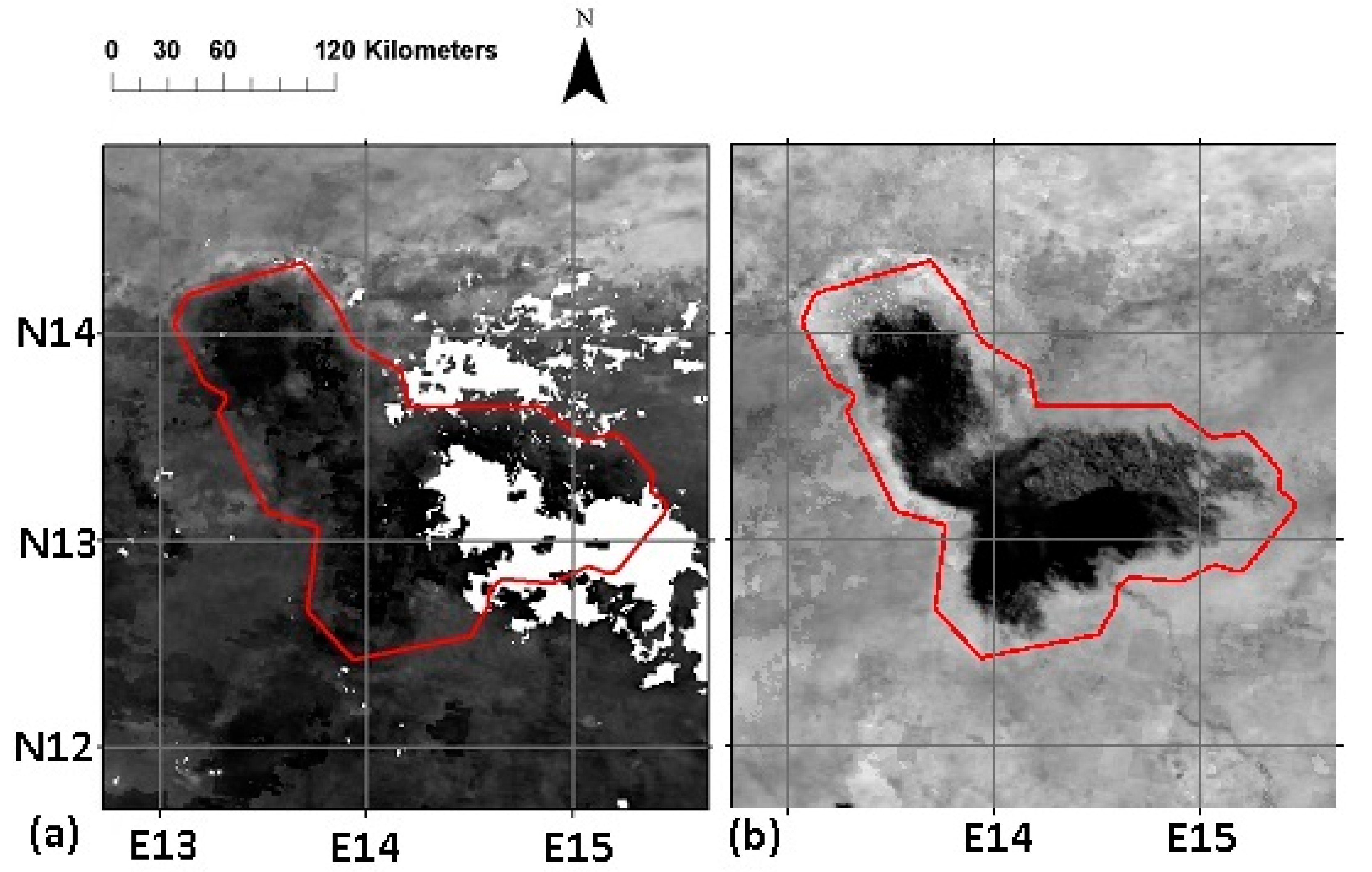
This section presents the results related to our investigation of Lake Chad total surface water area. The technique used in this study to measure the total surface water area of Lake Chad with LST measurements is severely limited by the need to use it only under dry conditions to avoid confusing soil moisture with flooded area and experiencing data loss (
Figure 4). Note the extensive area of cool temperatures (dark areas) during the wet season and the areas of data loss (white areas) in
Figure 4a and compare this with the dry season (
Figure 4b).
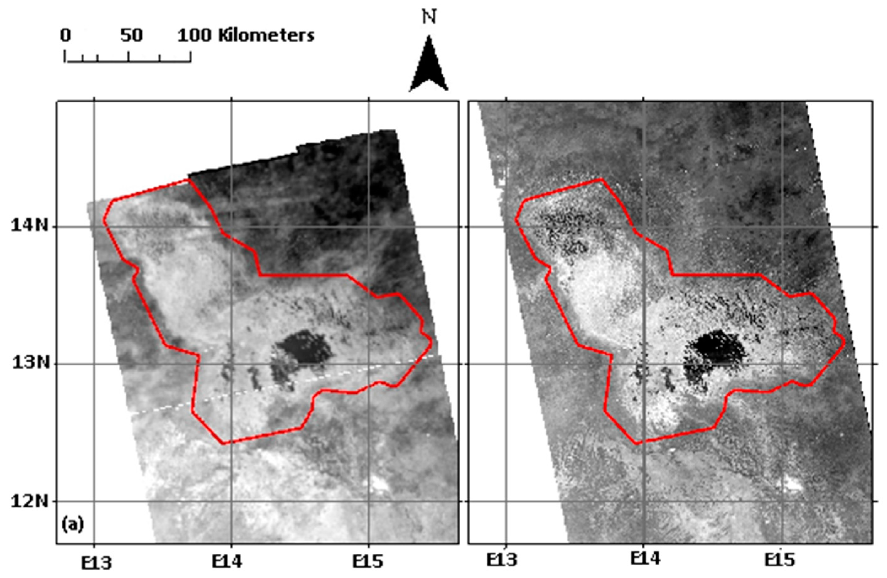
Use of C-band radar during the wet season seems to present a similar problem by failing to distinguish between soil moisture and flooded vegetation; notice in
Figure 5a (wet season) the boundaries of the lake are not as clear as in
Figure 5b (dry season). However, there are applications such as measuring total surface water area in the Sudd, or the Niger inland delta, or the Okavango Delta, that would also likely benefit from using both LST and radar remote sensing approaches during their dry seasons.
In the comparison of total surface water area from Sentinel-1a C-band radar with that from MODIS LST, we found a very low difference (less than 2 percent on average).
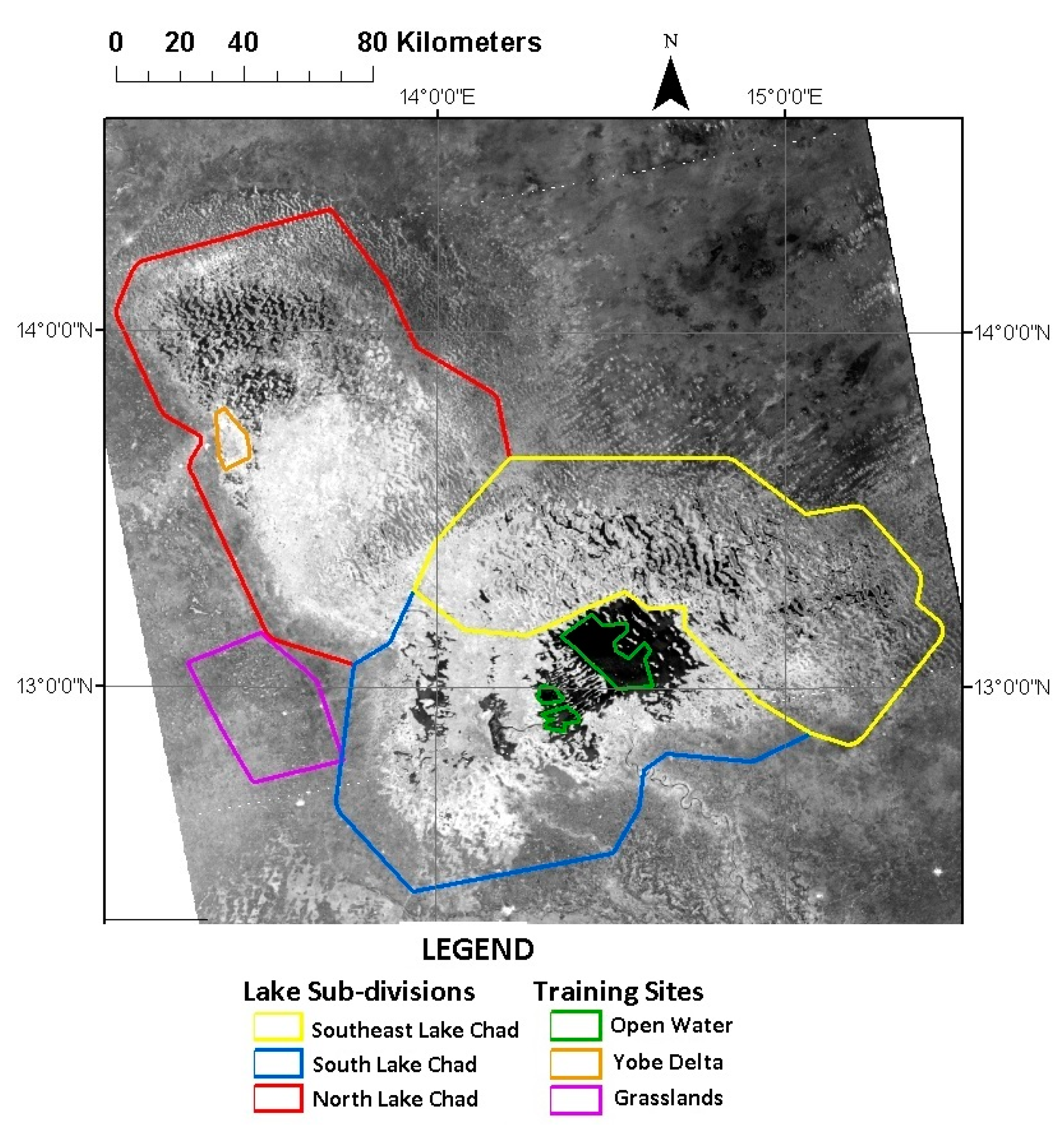
For each of the three regions and each of the 18 pairs of data sets, we determined the total surface water area calculated using the radar data and the LST data, and the percent difference between the two. We conclude that the surface water area calculated using the LST data is considerably more (31% on average) in Southeast Lake Chad, considerably less in North Lake Chad (19% on average), and very similar in South Lake Chad (0.3% greater on average); (
Table 2). The fact that the average area for the total lake is very close (within 2 percent) for the two different methods appears to be entirely coincidental. We found that within each subdivision of the lake, the differences between image pairs (LST and radar) appeared to be random, with no systematic pattern within or across the subdivisions as a function of time.
There is a substantial publication record (e.g., [
22,
23,
24,
25]) for the use of radar data for mapping wetlands including flooded vegetation. Wilusz et al. (2017) [
22] found that “low resolution C-band SAR imagery shows promise for long term study of Sudd wetland flood dynamics.” From a remote sensing perspective, the Sudd and Lake Chad have many similarities, and application of a successful technique in one area should encourage trial of that technique in the other. Radar has the advantage over LST of a relatively extensive history of use for mapping flooded vegetation. According to [
24], “SAR (Synthetic Aperture Radar) has many characteristics that make it ideal for mapping and monitoring water and wetlands over time.” According to [
26], “What is evident throughout the recent literature is that multidimensional radar data sets are attaining an accepted role in operational situations needing information on wetland presence, extent and conditions.” According to [
27], “Because of the strength of penetrating vegetation canopy and acquiring ground information all day without the limitation of clouds, radar data … are uniquely suited to identify and monitor changes of soil moisture, (and) flooding … in wetlands.” Given the relative maturity of the radar approach vs. the LST approach, we decided to use the differences between radar and LST-based estimates for the three subdivisions to derive appropriate correction factors to adjust the LST-based total surface water area time series.
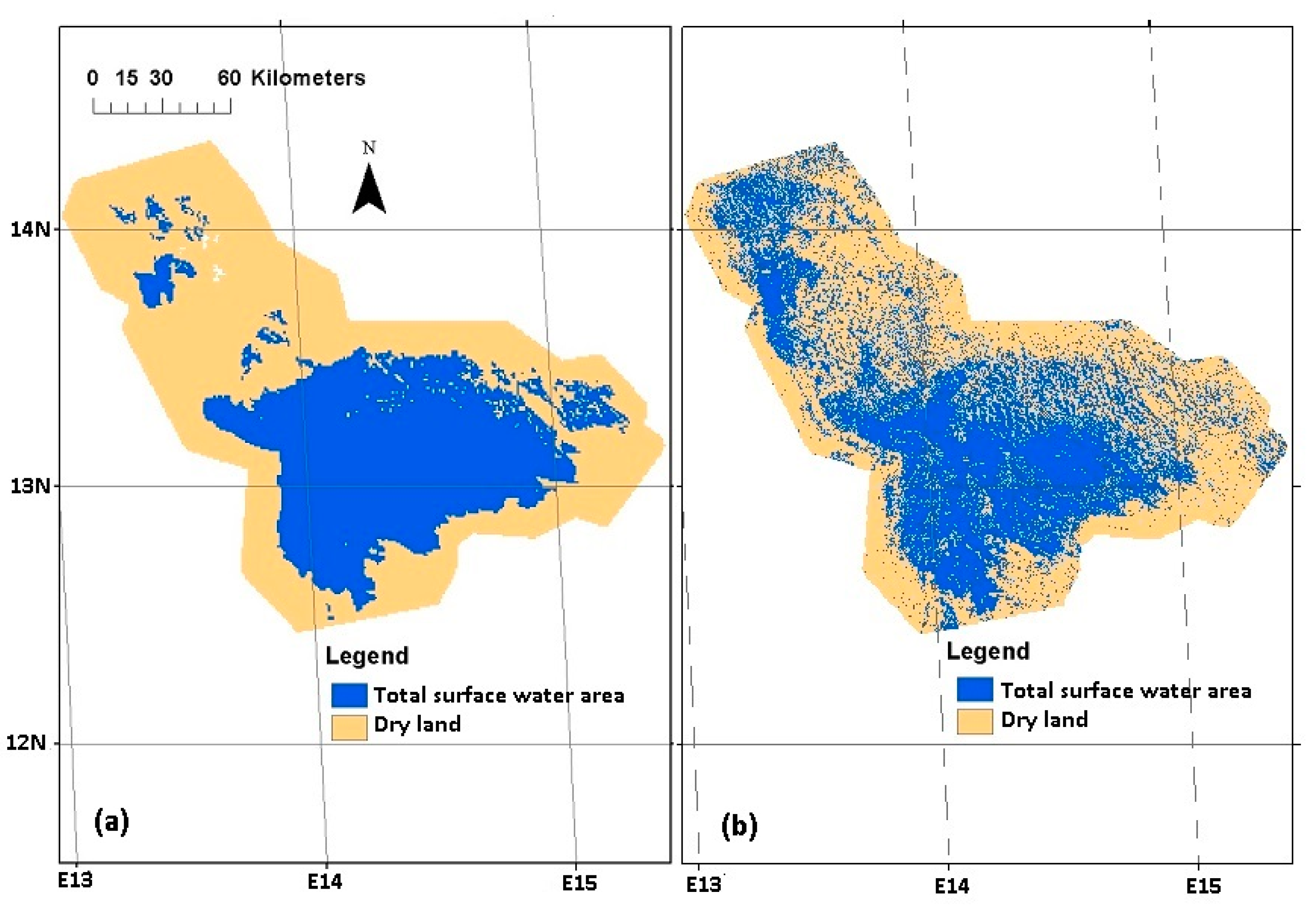
Figure 5 shows an example comparison of the LST and radar-derived water classifications. Note the spatial differences despite relatively close total surface water area estimates for these images. The example LST image (
Figure 6a) contains close to 12,300 square kilometers of total surface water area, while the corresponding radar image (
Figure 6b) contains approximately 12,100 square kilometers of total surface water area, a difference of approximately 2 percent.
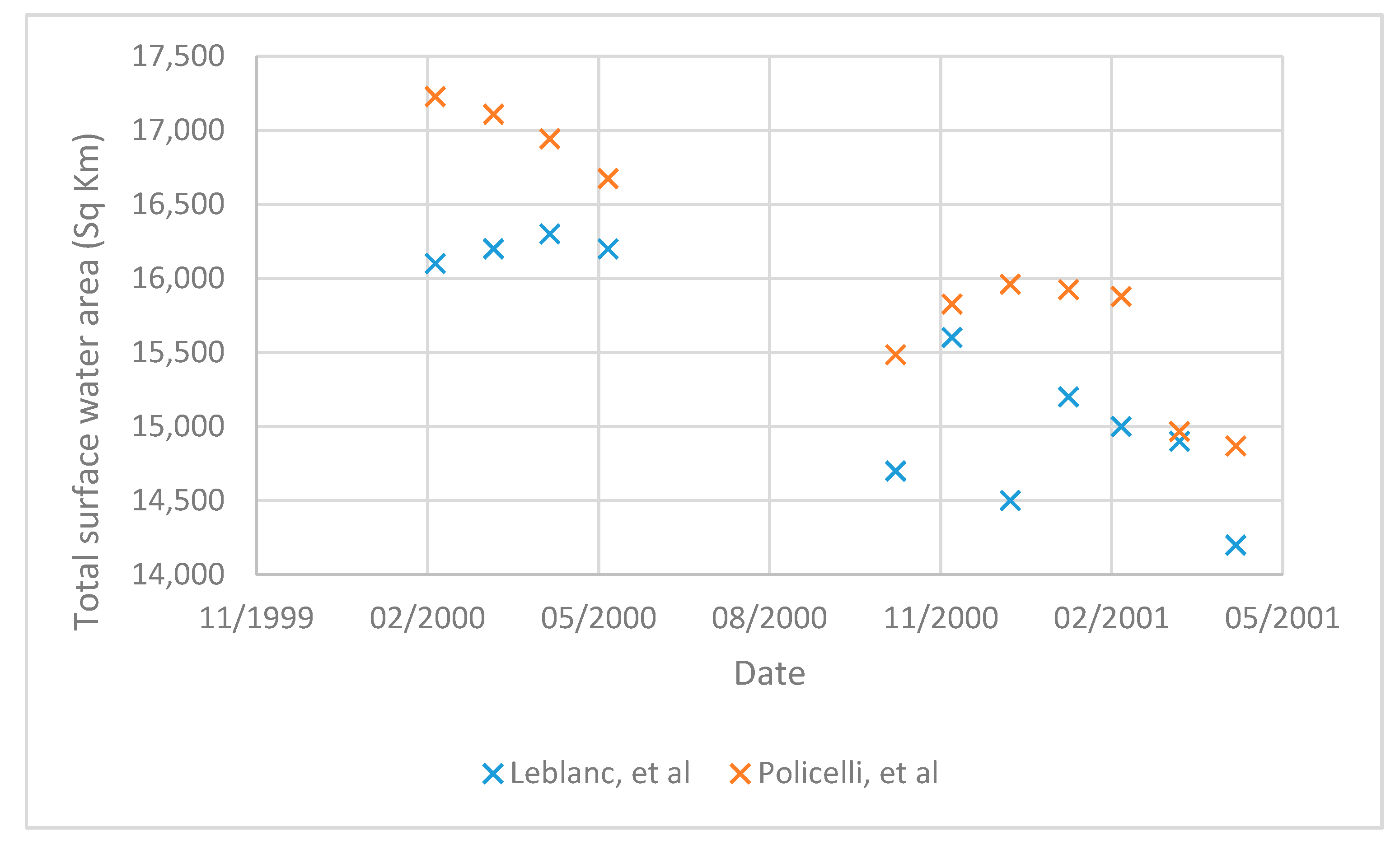
After adjusting the MODIS LST-derived lake area results using the differences with radar and then comparing the adjusted MODIS LST lake area results with the [
10] results using Meteosat LST, we found a low difference (our data was approximately 3 percent higher) during the period of overlap (dry season portion of March 2000–May 2001); see
Figure 7.
Based on the very similar results during the period of overlap, we concluded that it was appropriate to bias adjust the Leblanc data [
10], and present a single integrated time series of the two data sets approximately doubling the period of lake total surface water area time series. In
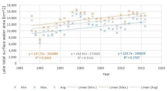
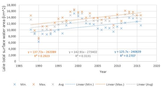
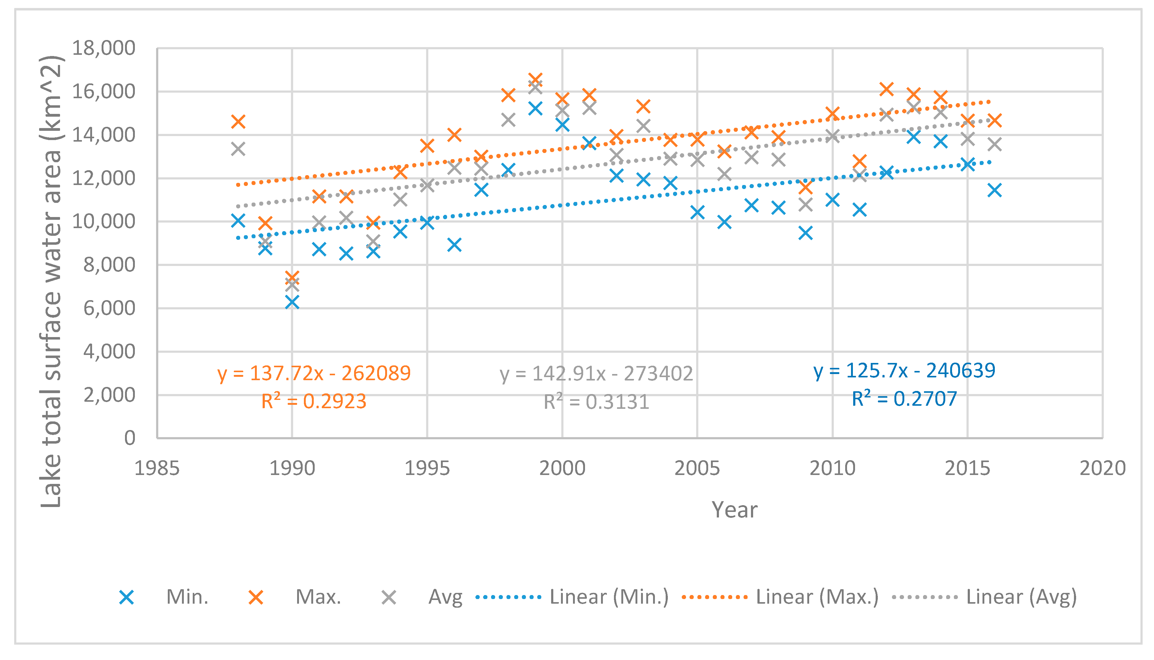
Figure 8, we plot the mean, maximum and minimum annual lake areas for each year (values are monthly), along with the mean, maximum, and minimum trend lines. Note that a given year represented on the graph corresponds to the dry season (November through May) starting in that year.
The general trend for the average total surface water area of the lake (
Figure 8) has been an increase of approximately 143 km
2 per year (slope of the average trend line). The R-Square value of the average trend line is 0.31 indicating high variability relative to the linear trend line. The slopes and the R-Square values are slightly lower for the maximum and minimum trend lines. A sinusoidal fit to the data is suggested by
Figure 8 (with periodicity between 11 and 13 years) and may be the result of large-scale climate oscillations. The El Nino phase of ENSO has a known influence on Lake Chad water level variability [
28]. However, “a much deeper understanding of the effect of other oceanic conditions like Atlantic Multidecadal Oscillation (AMO), Indian Ocean, and Mediterranean (oscillations) at different time-scales on Sahel precipitation is needed for a complete picture” [
28] of Lake Chad level variability.
The 25th percentile of total surface water area is approximately 11,700 square kilometers, the 50th percentile is approximately 12,900 square kilometers, and the 75th percentile is approximately 14,400 square kilometers. The time series exhibits a sharp decrease in the first two years, followed by a rise from 1990 to 1999, and then declining to 2009, rising to 2012, and a short, moderate decline since then.
The data show that, for the dry season, November is the month with the smallest lake total surface water area on average and the highest lake total surface water area occurs in March on average (
Table 3). There is considerable variability for each month.
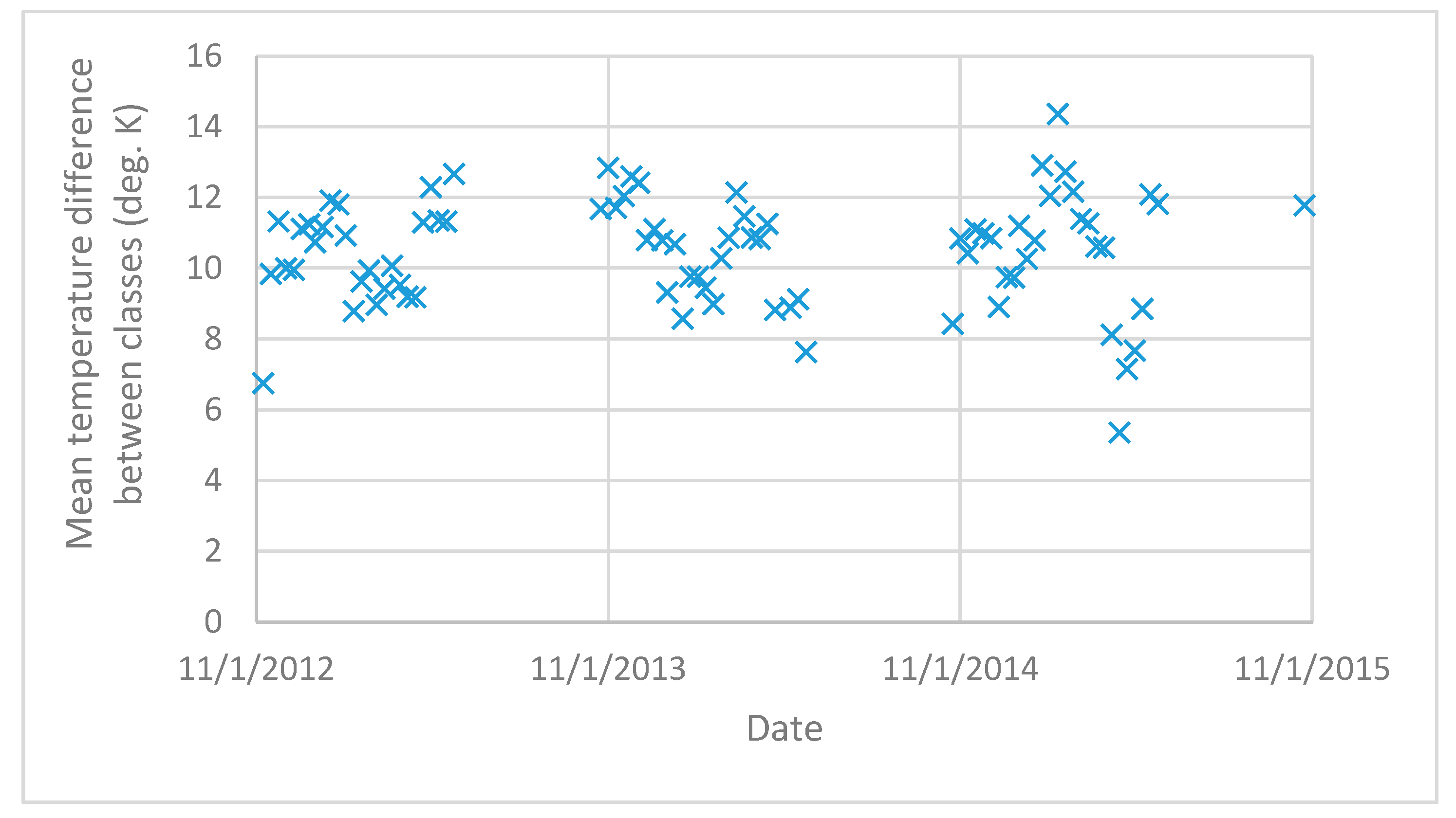
During the 2-class unsupervised classification of the MODIS LST data, we found that there was a substantial difference in the mean temperature between the two classes. As can be seen from
Figure 9, the mean temperature of the dry land class ranges between 5 and 15 degrees Kelvin above the average of the surface water class. This temperature difference provides a level of confidence that the two classes are sufficiently different to separate clearly. The maximum of the average surface water temperature was 310 degrees Kelvin (17–24 May 2010), and the minimum of the average surface water temperature was 292 degrees Kelvin (9–16 January 2002). The maximum of the average land surface temperature was 324 degrees Kelvin (17–24 May 2010), and the minimum of the average land surface temperature was 300 degrees Kelvin (1–8 January 2015). Again, only dry season data was used because of cloud contamination, data loss, and ambiguities between wet soil and inundated areas during the wet season.
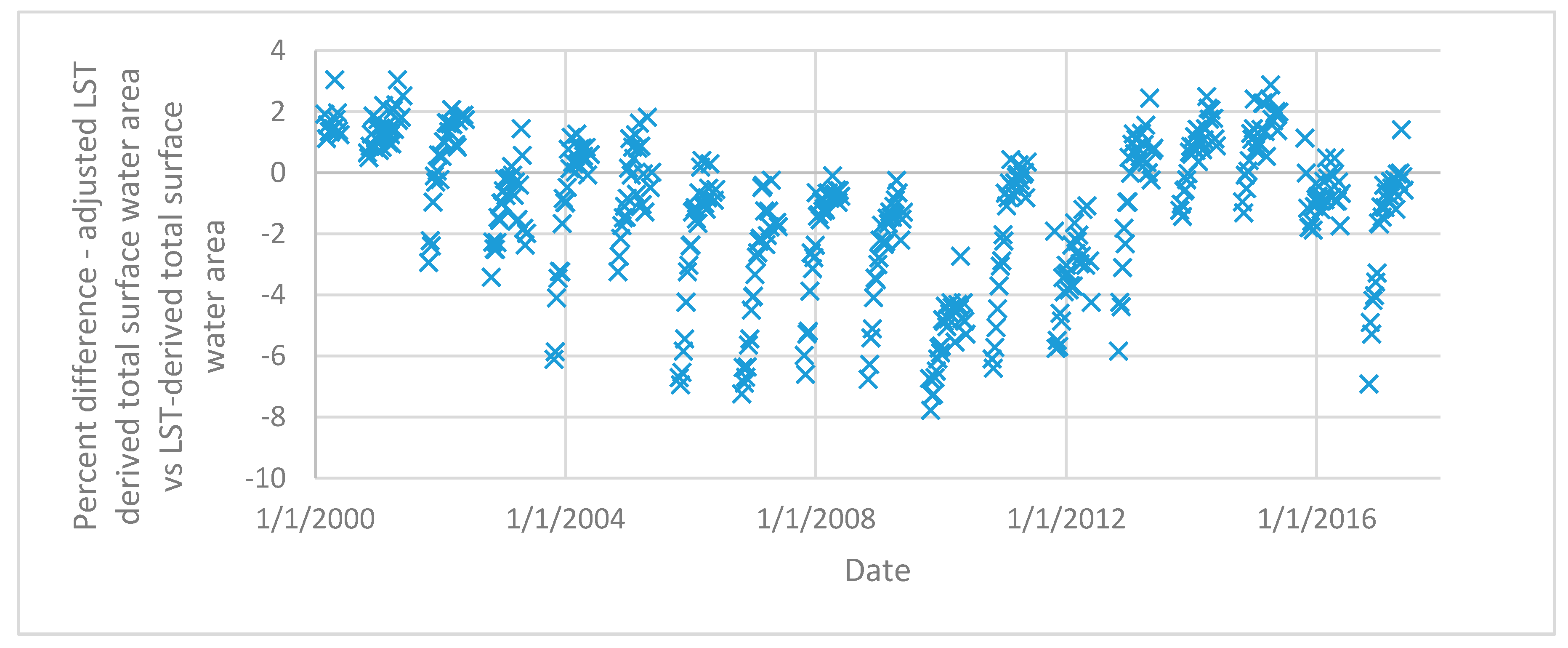
For the adjustment of the MODIS LST-derived total surface water area due to spatial disagreement with the radar data, we found that despite significant adjustments to the sub divisions of the lake, the average lake total surface water area was not changed greatly relative to the initial LST results. The average change of the total surface water area after adjustment of the sub divisions was about −1 percent, while the maximum change was about −8 percent.
Figure 10 presents a time series of the change. Both the time series in
Figure 10 and in
Figure 8 have a down-up-down pattern of approximately the same shape since 2000, so there appears to be a tendency towards positive bias for unadjusted MODIS LST-derived total surface water area when dry season lake levels are high and a tendency towards negative bias when lake levels are low.
4. Discussion
Use of the NASA MODIS Land Surface Temperature product has allowed us to extend the time series of Lake Chad’s total surface water area by about 15 years, updating and approximately doubling what was previously available. Having this time series helps us answer some fundamental questions about the dynamics of the lake including “what is the average total surface water area of the lake?” and “is the lake shrinking or growing?”
There are many challenges associated with estimating the total surface water area of Lake Chad; chief among them are the apparently extensive amount of flooded vegetation, which cannot be identified as containing water using optical remote sensing instruments. Leblanc et al. (2011) [
10], citing work by [
7,
29], subscribe to the idea that, “the transition from an ‘Average’ to a ‘Small’ Lake Chad in 1973 … was accompanied by the development of aquatic vegetation which now dominates the inundated area of Lake Chad”. To get an accurate accounting of the lake’s total surface water area, it is necessary to measure both the open water and the area covered by aquatic or “flooded” vegetation. Any approach that ignores this is bound to significantly underestimate the total surface water area of the lake. We have chosen to use LST and radar remote sensing datasets, as these approaches are inherently able to retrieve information beneath modest canopy coverage. It appears that surface water area under vegetation cover is often left out of consideration of the area of Lake Chad. The main cause of this oversight is likely the challenge of using remote sensing techniques to estimate the area of flooded vegetation associated with the lake. Though they do not provide any detail on their methods, the World Lakes Database of the International Lake Environment Committee’s estimate [
13] that Lake Chad covers just 1540 km
2 is likely an example of this.
Other challenges include (1) the lack of ground-based measurements of the Lake Chad water extent, which precludes validation of the remote sensing approach using in situ data; and (2) the relatively coarse resolution of the LST data available, which makes it difficult to get accurate areas for the small bodies of water associated with the lake in northern and southeastern Lake Chad.
The results of [
10], using Meteosat-based LST compare well with the overlapping period of adjusted MODIS LST-based results from this study; the Meteosat data is three percent lower on average. This similarity is to be expected because similar methods were used, however different LST data were used for the two sets of results, and Sentinel-1a C-band radar data were used to adjust the spatial biases in the MODIS LST data used in this study. The study by [
10] did not compare their results with other remote sensing approaches, though they did have one in situ observation. Additionally, the resolution of the LST data (1 km) was higher for this study than for the [
10] study (5 km), which should tend to give this study a better measurement of total surface water area. Atmospheric conditions such as clouds and dust have the potential to impact measurements of total surface water area for both the MODIS and Meteosat-based LST approaches, though this has been mitigated by several methods including the use of dry-season data only and monthly averaging of data without significant cloud coverage.
According to [
3], Lake Chad reached 14,000 square kilometers in April 2013. This is within close to ten percent of our figure of 15,600 square kilometers for the same month.
The results from [
4] did not compare well with the results from this study. In general, the results from the current study are 2 to 3 times higher than the peak areas from [
4]. The study by [
4] used near-infrared bands to detect water, though this method will only detect open water. While [
4] notes that some surface water area may be “masked by perimeter vegetation”, she does not mention the possibility of extensive masking by aquatic vegetation as cited by [
10], and her values of total surface water area are considerably lower than for [
10] and this study.
Because the reports of long term changes to Lake Chad described in the Introduction cover different time spans, they cannot be directly compared to our results, though it is worth mentioning that [
9,
11,
12] show a large shrinking of the lake, and the results of [
10] and this study show a modest net growth of the lake. On the other hand, indications of increased surface water area, rainfall, lake elevation, and flow to the lake by [
4,
13,
15,
16] are all consistent with a net growth of the lake during the period of our research.
As an example of model performance compared with our observation-based approach, Gao et al. [
6] uses the Variable Infiltration Capacity (VIC) hydrological model [
30] to estimate the total surface water area of Lake Chad from 1952 to 2006. From the late 1980s to 2006, they show a net rising trend in lake total surface water area, as does this study for the same period. In 1990 [
6] calculates a peak area of approximately 5000 square kilometers (compared to our value of 7400 square kilometers); in 2000 they calculate a peak area of approximately12,500 square kilometers, (compared to our value of 15,600 square kilometers) and in 2005 they calculate a peak area of approximately 10,000 square kilometers (compared to our value of 13,800 square kilometers). While the absolute values are very different, the trends are similar. The modeling approach has the advantage that total lake surface area can be forecast and wet season total lake surface area can be calculated. On the other hand, we expect observations of total lake surface area to be more accurate than calculation of area by a hydrological model, especially given the uncertainties of rainfall datasets over Africa [
31], and the complex topography of the lake area.
Wilusz et al. (2017) [
22] used only C-band radar for their analysis of the Sudd wetland flooded area in South Sudan. The radar data is not affected by clouds and can be taken during the day or night. While their results did not require adjustment, they were limited to five years of available data (compared to twenty-eight years in our study). In our analysis, we calculated total surface water area using two remote sensing methods, C-band radar and LST. The C-band radar and LST methods agree well in southern Lake Chad, which contains a great deal of open water. However, when determining total surface water area in north and southeast Lake Chad, two competing factors (i.e., penetration of canopy and spatial resolution) resulted in a difference between the C-band radar and the LST method. In north Lake Chad, where there is a large extent of vegetated water, the LST method underestimates total surface water area relative to the radar. C-band radar has the ability to penetrate vegetation canopy to some extent and detect surface water in flooded vegetation in addition to open water [
19]. While the use of unsupervised classification on LST data can identify surface water through gaps in the canopy, this method can be negatively affected by the warmer canopy even though it is moderated by the cooling effect of vegetation through transpiration and other mechanisms [
32]. In southeast Lake Chad, the landcover is mainly a mix of dunes and open water. The coarser resolution of the LST method tends to classify a large area of these mixed pixels as water due to the large difference between water and land surface temperatures, which leads to an overestimate of surface water area in this region relative to the radar. We adjusted for these under- and over- estimates by using a correction factor for each of the three sub-divisions for the data from this study and then used the adjusted data to bias correct the data from [
10].
Extension of the Lake Chad area time series can be continued using MODIS LST as long as either MODIS on the NASA Terra or Aqua satellites is operating. However there is now another option with the LST product from the VIIRS sensor on the NASA Suomi NPP satellite, and soon to be available from the VIIRS sensors on the NOAA JPSS series of operational satellites. The VIIRS sensor provides LST data at a higher resolution (0.75 km) than the MODIS sensor or the Meteosat-based sensor [
33].
5. Conclusions
In this study, we compared the Land Surface Temperature (LST) method and the radar method of measuring Lake Chad’s total surface water area (open water plus flooded vegetation), assumed that the widely used, higher resolution radar method is more reliable, and adjusted the longer LST record using data from the radar method. We used 8-day NASA MODIS LST data from March 2000 to May 2017, ESA Sentinel-1a C-band radar data acquired from April 2015 to May 2017, and Lake Chad total surface water area data from a previous study for November 1988 to May 2001.
To identify the total surface water area of Lake Chad, we examined LST and radar datasets from which we derived similar overall areas, although with significant differences in the spatial coverage of each. The comparison of the LST and radar datasets likely suffered from the fact that it was necessary to use 8-day MODIS LST data to effectively clear clouds and provide complete datasets, as compared to the use of single day radar data, the fact that the radar data are much higher resolution (100 m resampled for radar, and 1 km for the LST), and the ability of radar to penetrate modest canopy coverage. C-band radar products from Sentinel-1a are relatively new, and there is no close analog on other platforms that was readily available for this study, with the exception of Sentinel-1b, which has an even shorter data record.
The availability of radar data from Sentinel-1a for a portion of the LST record enabled us to adjust the LST-derived total surface water area estimates and extend the existing total surface water area record for Lake Chad. A picture has emerged of the past 28 years of Lake Chad’s total surface water area that is generally increasing, at an average rate of 143 square kilometers per year and with a great deal of variability (described above). For the dry season of 1988–1989 through the dry season of 2016–2017, we find that the maximum monthly average total surface water area of the lake was approximately 16,800 sq. km (February and May 2000), the minimum monthly average total surface water area of the lake was approximately 6400 sq. km (November 1990), and the average of the total monthly surface water area was approximately 12,700 sq. km. The 25th percentile of total surface water area was approximately 11,700 square kilometers, the 50th percentile was approximately 12,900 square kilometers, and the 75th percentile was approximately 14,400 square kilometers.
This research has addressed important questions about the size and trend of Lake Chad’s total surface water area. Future efforts at mapping and calculating the area of Lake Chad would greatly benefit from in situ measurements, as well as the continuing radar and LST records.


