Article

The Impact of Tourist Traffic on the Condition and Cell Structures of Alpine Swards

by
Marlena Kycko
1,*,
Bogdan Zagajewski
1,
Samantha Lavender
2,
Elżbieta Romanowska
3 and
Magdalena Zwijacz-Kozica
4
1
Department of Geoinformatics, Cartography and Remote Sensing, Faculty of Geography and Regional Studies, University of Warsaw, Krakowskie Przedmieście 30, 00-927 Warsaw, Poland
2
Pixalytics Ltd., 1 Davy Road, Plymouth Science Park, Derriford, Plymouth, Devon PL6 8BX, UK
3
Department of Molecular Plant Physiology, Faculty of Biology, University of Warsaw, Miecznikowa 1, 02-096 Warsaw, Poland
4
Tatra National Park, Kuźnice 1, 34-500 Zakopane, Poland
*
Author to whom correspondence should be addressed.
Remote Sens. 2018, 10(2), 220; https://doi.org/10.3390/rs10020220
Submission received: 16 January 2018 / Revised: 27 January 2018 / Accepted: 30 January 2018 / Published: 1 February 2018
(This article belongs to the Special Issue Recent Progress and Developments in Imaging Spectroscopy)

Abstract

:
This research focuses on the effect of trampling on vegetation in high-mountain ecosystems through the electromagnetic spectrum’s interaction with plant pigments, cell structure, water content and other substances that have a direct impact on leaf properties. The aim of the study was to confirm with the use of fluorescence methods of variability in the state of high-mountain vegetation previously measured spectrometrically. The most heavily visited part of the High Tatras in Poland was divided into polygons and, after selecting the dominant species within alpine swards, a detailed analysis of trampled and reference patterns was performed. The Analytical Spectral Devices (ASD) FieldSpec 3/4 were used to acquire high-resolution spectral properties of plants, their fluorescence and the leaf chlorophyll content with the difference between the plant surface temperature (ts), and the air temperature (ta) as well as fraction of Absorbed Photosynthetically Active Radiation (fAPAR) used as reference data. The results show that, along tourist trails, vegetation adapts to trampling with the impact depending on the species. A lower chlorophyll value was confirmed by a decrease in fluorescence, and the cellular structures were degraded in trampled compared to reference species, with a lower leaf reflectance. In addition, at the extreme, trampling can eliminate certain species such as Luzula alpino-pilosa, for which significant changes were noted due to trampling.

Graphical Abstract

1. Introduction

Mountain vegetation grows under adverse environmental conditions, which leads to the development of specific adaptations (pigment content, plant tissue structure, leaf wax covers, etc.) to survive at the fringe of life. All these adaptations have a direct impact on reflectance, which can be quantified using hyperspectral techniques [1]. Non-invasive methods should play a leading role in highly protected areas but have to be supported by biophysical variables [2,3]. For example, remote sensing enables the identification of plants and vegetation communities in mountainous areas [4,5], and the mapping or monitoring of vegetation can be carried out at various spatial scales depending on the sensors used [6]. The state of cell structures, photosynthetically active pigments, water, lignin and cellulose content determines the spectral reflectance curve in different parts of the electromagnetic spectrum [7]. In addition, the relationship between absorbed and scattered photons allows an exploration of the stress resistance mechanism(s) according to species properties [8,9,10].
The vulnerability of vegetation to trampling damage is expressed by three indices: resistance (ability of vegetation to resist change when trampled), resilience (ability of vegetation to recover following the cessation of trampling) and tolerance (ability of vegetation to tolerate a cycle of disturbance and recovery) [11,12]. Reductions in cover or abundance of vascular plants have repeatedly been shown to be a response to trampling [13,14,15], and several studies show decreases in shrub cover [16,17,18]. Mechanical traits, including leaf toughness, root strength and stem flexibility have also been observed to play a key role [19,20,21]. Studies have shown that trampling-resistant species that grow well, alongside species that are very sensitive [22,23], are constrained by the packed earth of trampled land, which is a barrier to germination and thus plant regeneration [24]; soil bulk density of trampled and untrampled soils increases with increasing exposure [25]. Low-intensity anthropopression may increase plant resistance and defensive physiological adaptations, and at higher intensities damages fragile biosphere cover.
The monitoring of vegetation should be based on photosynthetically active pigments, especially chlorophylls and carotenoids (antheraxanthin, β-carotene, lutein, neoxanthin, violaxanthin, and zeaxanthin). In addition, the relationship between chlorophylls and carotenoids are indicators of the short- and long-term stress of plants [26]. A key element of chlorophyll molecules is the light re-emitted during the return from an excited to non-excited state (chlorophyll fluorescence); it is used as an indicator of photosynthetic energy conversion in higher plants. Therefore, chlorophyll fluorescence yield provides quantitative information not only on steady-state photosynthesis but also on various mechanisms for protection against stress-induced damage [27]. The fluorescence emission intensity is sensitive to changes in the photosynthetic apparatus; in terms of both the health and function of the photosynthetic process [28]. The use of fluorescence determines the actual damage of cellular structures, which is reflected by the quantity of light-related reaction products in the plant [29]. Coupling fluorescence measurements with other non-invasive techniques such as gas exchange, thermal imaging and absorption spectroscopy can provide insights into stress conditions before visible external symptoms such as wilting, necrosis and chlorosis are present [30]. Such methods should be supported by hyperspectral imaging techniques [31], especially airborne and Unmanned Aerial Vehicle (UAV) based, to better understand spatio-spectral patterns [32,33]. For example, hyperspectral data (the Compact Airborne Spectrographic Imager—CASI, the Reflective Optics System Imaging Spectrometer—ROSIS, the Digital Airborne Imaging Spectrometer—DAIS-7915, and terrestrial spectrometer) and bio-radiometric measurements (Leaf Area Index—LAI) on vineyard fields [34,35] were used. The amount of chlorophyll a and b and carotenoids in vegetation was estimated, as well as by remote sensing vegetation, determining the state of the vines. The authors determined that some of the best-performing (R2 approximately 0.50) for variability of the ratio of chlorophylls to carotenoids are Structure Insensitive Pigment Index (SIPI) and Photochemical Reflectance Index (PRI), while the best indicators for chlorophyll content correlation are (R2 approximately 0.80–0.90) Zarco and Miller (ZM), Gitelson and Merzlyak (GM1, GM2), Modified Chlorophyll Absorption in Reflectance Index (MCARI), Transformed Chlorophyll Absorption in Reflectance Index (TCARI), Optimized Soil-Adjusted Vegetation Index (OSAVI), MCARI/OSAVI, and TCARI/OSAVI [35]. Adding fluorescence to data obtained from UAV on the example of citrus trees, the authors tried to determine water stress using chlorophyll fluorescence and PRI measurements. Chlorophyll fluorescence was calculated from the micro-hyperspectral imagery with the method tracked stress levels, obtaining R2 = 0.67 (p < 0.05) with stomatal conductance, and R2 = 0.66 (p < 0.001) with water potential [36]. The newest hyperspectral scanners for UAVs allow registration of the full range of the electromagnetic spectrum (including the Shortwave Infrared SWIR, e.g., HySpex for UAV) [35,36]. This is particularly important for mountain areas, where the weather conditions are unstable.
The aim of this study was to present a field-based method for non-invasive analysis of the condition of the dominant sward species surrounding the most frequented alpine tourist trails in the Tatra National Park (UNESCO Man and the Biosphere Reserve), which is one of the most visited natural mountain parks in Poland (around 500,000 tourists explore the research area every summer). As the main source of information, ASD FieldSpec 3/4 hyperspectral measurements were used to analyze interactions between the electromagnetic spectrum and the morphology and physiology of plants. To confirm the variation in vegetation presented by means of remote sensing, the biophysical variables chlorophyll content in the leaves, chlorophyll and fluorescent in vivo, absorption of photosynthetic active radiation, and transpiration processes were used. It is extremely important to use chlorophyll and fluorescence in vivo, which shows us the physiological condition of live tissues and is an indicator of photosynthetic energy conversion in plants. The goals of the analyses were: showing the impact of trampling on alpine swards, identifying the species sensitive and resistant to trampling, and assessing their physiological condition. The species level is extremely important, since the vegetation reacts differently to the process of trampling; some species are more at risk than others, resulting in the disappearance of a valuable natural resource. Such analyses support the management processes of reconstruction and regeneration of the vegetation cover, especially in terms of retaining fractional vegetation cover. Therefore, hyperspectral remote sensing and chlorophyll fluorescence methods are a promising non-invasive tool for monitoring hiking trails and mountainous areas, and future studies could be based on airborne hyperspectral images.

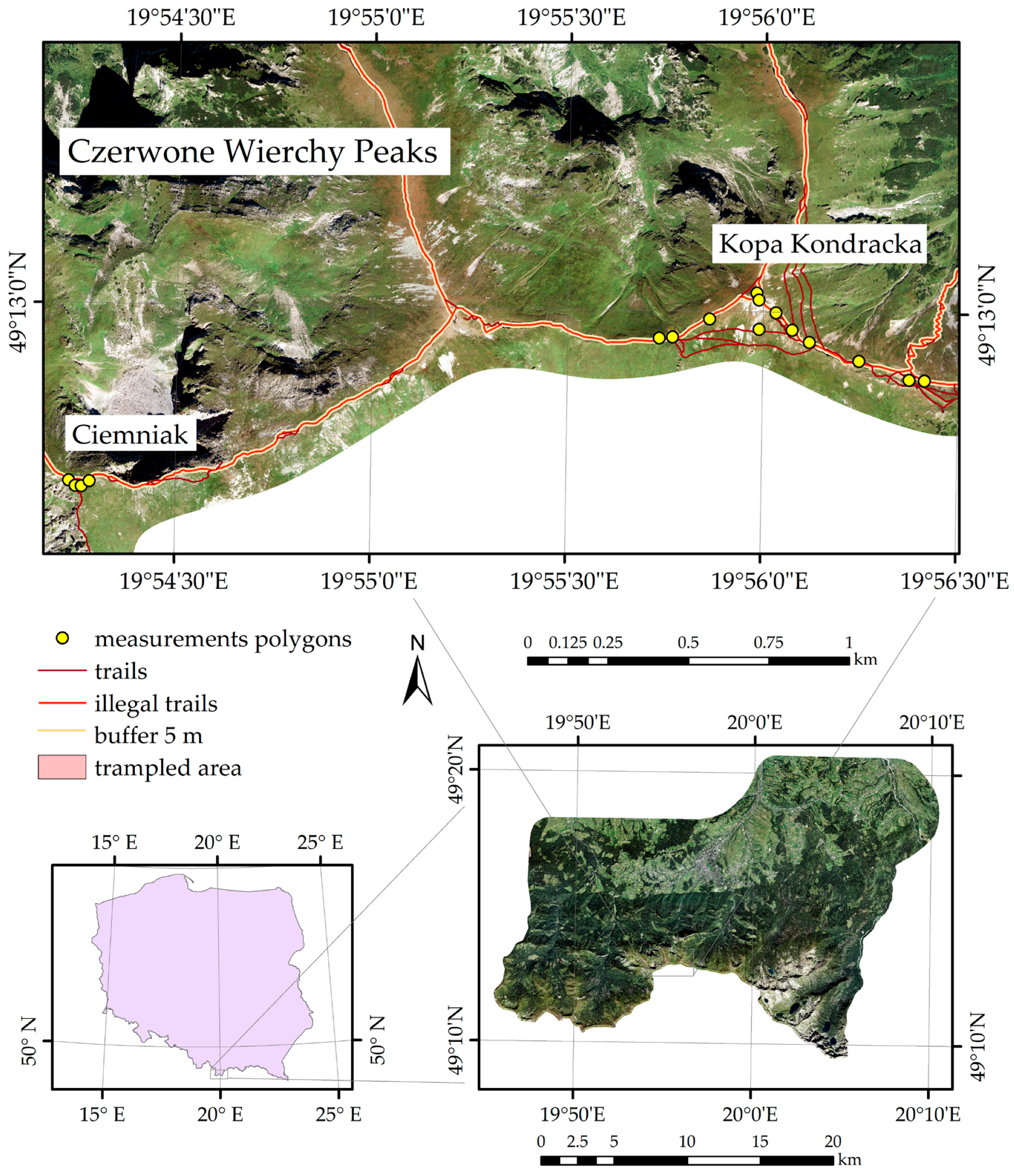
2. Study Area and Research Objects

The Tatra test site is located within the Man & Biosphere Reserve, encompassing alpine and subalpine zones of the Polish and Slovak Tatra National Park (TPN and TANAP). The area (49°10′30″ to 49°16′00″N and 19°45′30″ to 20°07′30″E) covers approximately 110 km2 and is located at an altitude range of 1500–2300 m above sea level (a.s.l). The central parts of the Polish High Tatras (Kasprowy Wierch region and Czerwone Wierchy Mountains) were investigated (Figure 1).
The core of the massif is composed of sedimentary rocks (limestone and dolomites of the Middle Triassic), with the tops covered by a mantle of crystalline rocks (granites and gneisses). The Czerwone Wierchy name comes from the red-brown color of the slopes, which results from a plant called Juncus trifidus fading to red in the autumn; and often as early as mid-summer. The altitude also results in the occurrence of Oreochloa disticha and Festuca picta. Due to the varied geological substrate, diverse vegetation is present, e.g., both the aforementioned plants can grow on calciphilous and acidophilic soils. Therefore, alpine swards are an excellent example of communities susceptible to change [34,35]. The research conducted so far [36] has revealed that species react differently to stress factors, depending on their morphology and the type of the cellular structures.
The study was conducted during August in both 2013 and 2014. Based on experience and previously conducted research, species were selected to include the greatest percentage of high-altitude communities [35]. After consultation with field scientists of phytosociology, and selection using a map of the main vegetation species in this area, the following species were selected: Juncus trifidus, Agrostis rupestris, Luzula alpino-pilosa, Oreochloa disticha, and Festuca picta.
Trails are frequently visited by tourists, as evidenced by the large-scale destruction resulting from the tourist infrastructure (Figure 2). In 2014, TPN began revitalization of the area through the reconstruction of routes and their surrounding areas in order to reduce the impact of tourist traffic both in activating the erosion processes and in trampling vegetation, and also in order to enable regeneration of damaged vegetation (co-financed by the EU project No. POIS.05.01.00-00-398/12).

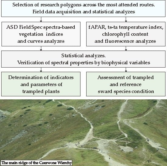
3. Materials and Methods

Although many mountain ecosystem vegetation communities are heterogeneous, to obtain a spectral signal from a single species at a time, measurements were taken within highly homogeneous alpine sward patches across the most crowded trails within the Czerwone Wierchy Peaks (Figure 2). The map of trampled and damaged areas was delivered by the Tatra National Park, and the initial selection of alpine sward locations was conducted with a vegetation map at a scale of 1:10,000 [37]. Then, following a detailed species analysis, Juncus trifidus, Oreochloa disticha, Agrostis rupestris, Festuca picta, and Luzula alpino-pilosa were selected. They are monocotyledonous plants with a similar growth type (clump forming) and belonging to the families Juncaceae and Poaceae. The Juncaceae family is represented by two species belonging to separate genera: Juncus trifidus and Luzula alpino-pilosa, while the Poaceae family contains Agrostis rupestris, Festuca picta and Oreochloa disticha. The main criterion for selection was a dominant presence within homogeneous patches in trampled zones (<5 m from a trail) and control areas (>5 m from a trail) in the same topographical habitats. A distance of 5 m was considered the maximum distance that tourists are likely to walk or stand away from the trail, because of the slope steepness. All polygons were located by the GPS Trimble GeoXT receiver with an accuracy that oscillated around 50 cm (real-time measurements, Figure 2, Table 1).
Each of the 16 polygons covered a few dozen homogenous patches of all investigated species (the number of patches was different for different polygons, but attempts were made to collect sets of trampled and reference patches for each species in every polygon). Every patch had a dimension of 1 m2, and all the terrain measurements were collected in the period from 10:00 to 14:00 with the same set of measurements performed:
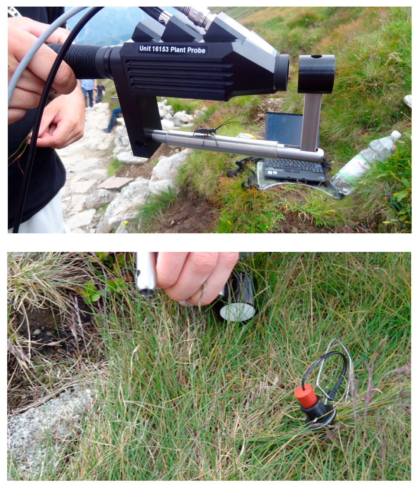
  • Hyperspectral properties of plants using an ASD FieldSpec 3/4 spectrometer fitted with a contact probe (ASD PlantProbe), operating in the range 350–2500 nm (ASD Inc., Longmont, CO, USA). The ASD PlantProbe uses an artificial light and closed chamber for data acquisition at the leaf-level, offering comparable results for all measurements within test areas during the field campaigns. The instrument was configured by taking 25 measurements of the Dark Current (DC), then 25 of a White Reference spectralon reflectance target (SG 33151 Zenith Lite) in the cap of the ASD PlantProbe, which was repeated before every plant patch (Table 1). The plant spectral properties were acquired from 25 independent plant measurements, which were averaged into one spectral characteristic (a spectral record) with 10 records acquired for one plant patch, i.e., totaling 250 measurements that affording a higher data objectivity (Table 1). The measurements were made directly on the leaves using a fiber cable (25° field of view (FOV)) placed in the ASD PlantProbe, which takes measurements from a one cm of FOV circle area of leaves in the ASD PlantProbe (Figure 3). All leaves were measured in the upper (5 measurements) and middle (5) parts of plants. In the case of narrow leaves, a set of touching leaves were used [32].
  • The fraction of accumulated radiation in the range of photosynthesis (fAPAR) [34] that is the total radiation used by the vegetation for photosynthesis, measured using an AccuPAR linear ceptometer at the canopy level. In each field course, two sets of the following Absorbed Photosynthetically Active Radiation (APAR) components were made: PAR0, amount of radiation reaching the surface of the plant; PARc, amount of radiation reflected by plants; PARt, amount of radiation that has penetrated the plants; and PARs, amount of radiation that has been reflected from the ground; this biophysical variable is directly related to the primary productivity of photosynthesis.
  • The temperature index, ts-ta, is the difference between ts (the plant surface temperature), and ta (the air temperature), which defines evapotranspiration and water stress (pyrometer IRtec MiniRay) at the canopy level. Ten independent measurements of ts and ta were made.
  • Chlorophyll content in leaves was measured as Chlorophyll Content Meter (CCM-200) at the leaf level. Twenty independent measurements were made.
  • Chlorophyll fluorescence—a Plant Stress Meter (PSM Mark II) fluorometer for the analysis of the actual state of the photosynthetic apparatus (the peak wavelength for the Far Red source is ~690 nm); fluorescence measurements were made for dark adapted leaves (20 min; Fv/Fm; Figure 3) as 10 independent measurements; the level of half rise-time (t½) using leaf clips. Measurements of chlorophyll fluorescence provide a useful probe of photosynthetic performance in vivo, and the extent to which performance is limited by photochemical and non-photochemical processes [38]. The parameters that determine the photosynthetic efficiency and state of photosynthetic apparatus are the maximum quantum efficiency of photosystem II (PSII) photochemistry (Fv/Fm, where Fm is maximal fluorescence; Fv is variable fluorescence equal to Fm-Fo; and Fo is minimal fluorescence) and t½ (half rise time from Fo to Fm, which indicates the size of antenna systems). Fv/Fm describes the photochemical efficiency of the PSII, i.e., the parameter most sensitive to stress factors. Fv/Fm represents the maximum quantum efficiency of PSII, if all capable reaction centers were opened, and so a value from 0.79 to 0.84 is the optimal value for many plant species, with lower values indicating plant stress [39,40]. In dark adapted plants (measured part of the leaf has been in the dark for an extended period of time before measurement), the electron transport chain is not active, whereas, in the light, all chlorophyll molecules are fully activated and transfers light energy to a reaction center.
The results of the spectrometric, bio-radiometric and fluorescence measurements were compiled. The spectral curves for each alpine sward species were analyzed using ANOVA (significance level of 0.05), with the spectral characteristics of trampled and reference vegetation used to verify which part of the spectral range showed the biggest difference in terms of pigments, cellular structures and water content.
Based on the spectral characteristics of the tested species, vegetation indices were calculated; mathematical relationships between spectral reflectance values in narrow, well-defined ranges allow more accurate analysis of vegetation parameters [40]. Selected statistical tests were performed to check if the data distribution was normal (Shapiro–Wilk test) and identify changes between trampled and reference vegetation. The choice was not accidental: the remote sensing vegetation indices chosen were those that showed the largest, significant percentage of changes for the studied plants. In addition, it was suggested that the indicators would not show strongly correlated information, and those that would significantly capture changes in the plant were selected, including dyes or water. Because all vegetation indices had a nonparametric distribution, to find statistically significant (p < 0.05 level) indicators Mann–Whitney U test was used to compare information for species in two types of polygons and the Spearman tests of correlation this data (nonparametric distribution). Based on previous research [32,37], the choice of indicators was based on statistically significant ranges of the spectrum for the analyzed species. The remote sensing vegetation indices chosen were those that in previous studies allowed observing any changes in vegetation. Then, remote sensing vegetation indices were designed, selected and calculated to provide a measure of the overall quantity and quality of the photosynthetic material, which is necessary for understanding the vegetation state:
  • Wide Dynamic Range Vegetation Index (WDRVI) [41], Soil-Adjusted Vegetation Index (SAVI) [42], Green Normalized Difference Vegetation Index (Green NDVI) [43], Greenness Index (GI) [44], and Red Edge Position Index (REPI) [45];
  • Modified Normalized Difference Vegetation Index 705 (mNDVI705) [46], Transformed Chlorophyll Absorption Reflectance Index (TCARI) [47], Modified Chlorophyll Absorption Ratio Index (MCARI) [48], Normalized Pigment Chlorophyll Index (NPCI) [49], Simple Ratio Pigment Index (SRPI) [50], and Normalized Phaeophytinization Index (NPQI) [51];
  • Photochemical Reflectance Index (PRI) [52], Structure Insensitive Pigment Index (SIPI) [50], and Xanthophyll Epoxidation State (XES) [53];
  • Normalized Difference Nitrogen Index (NDNI) [54];
  • Normalized Difference Lignin Index (NDLI) [54];
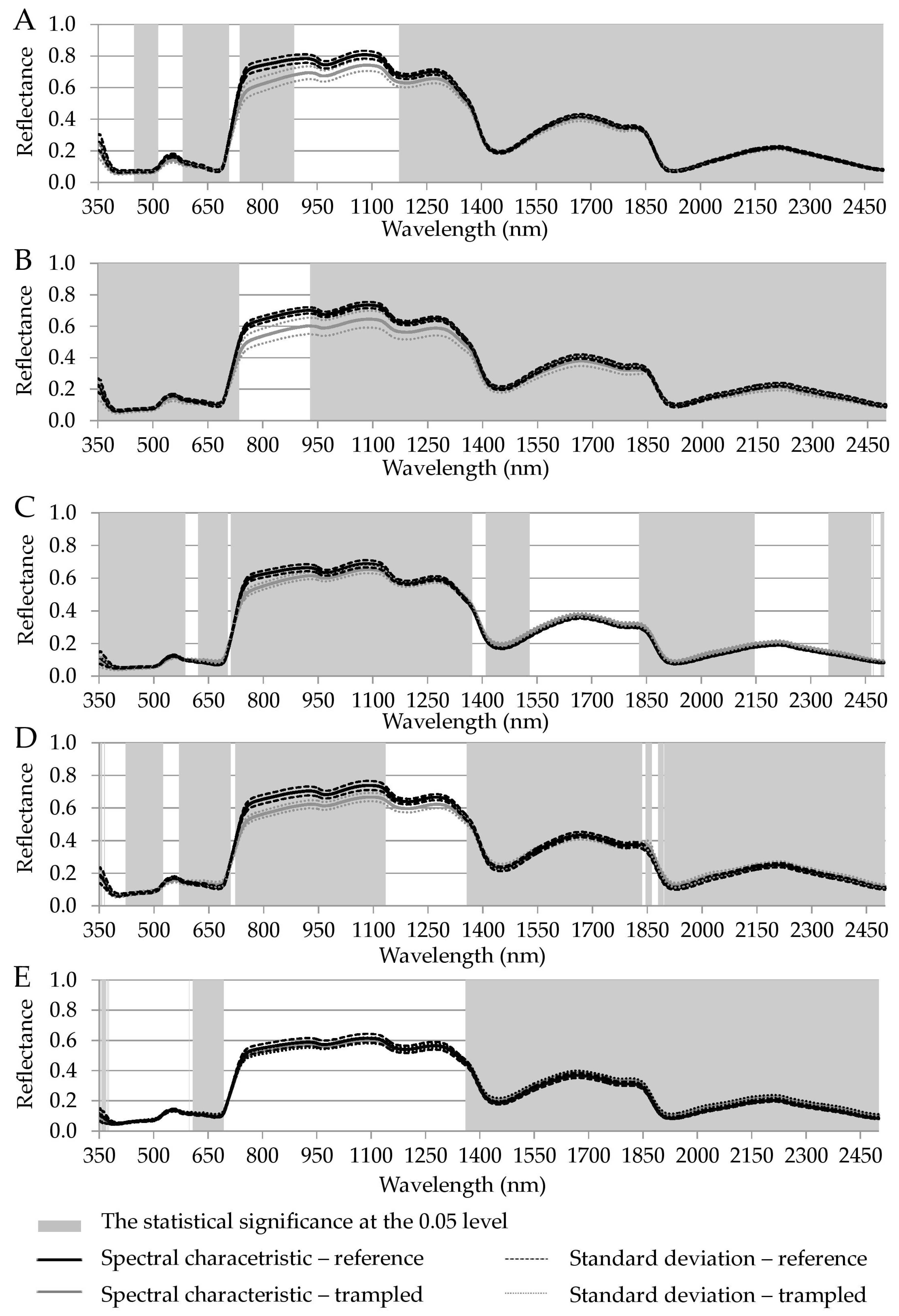
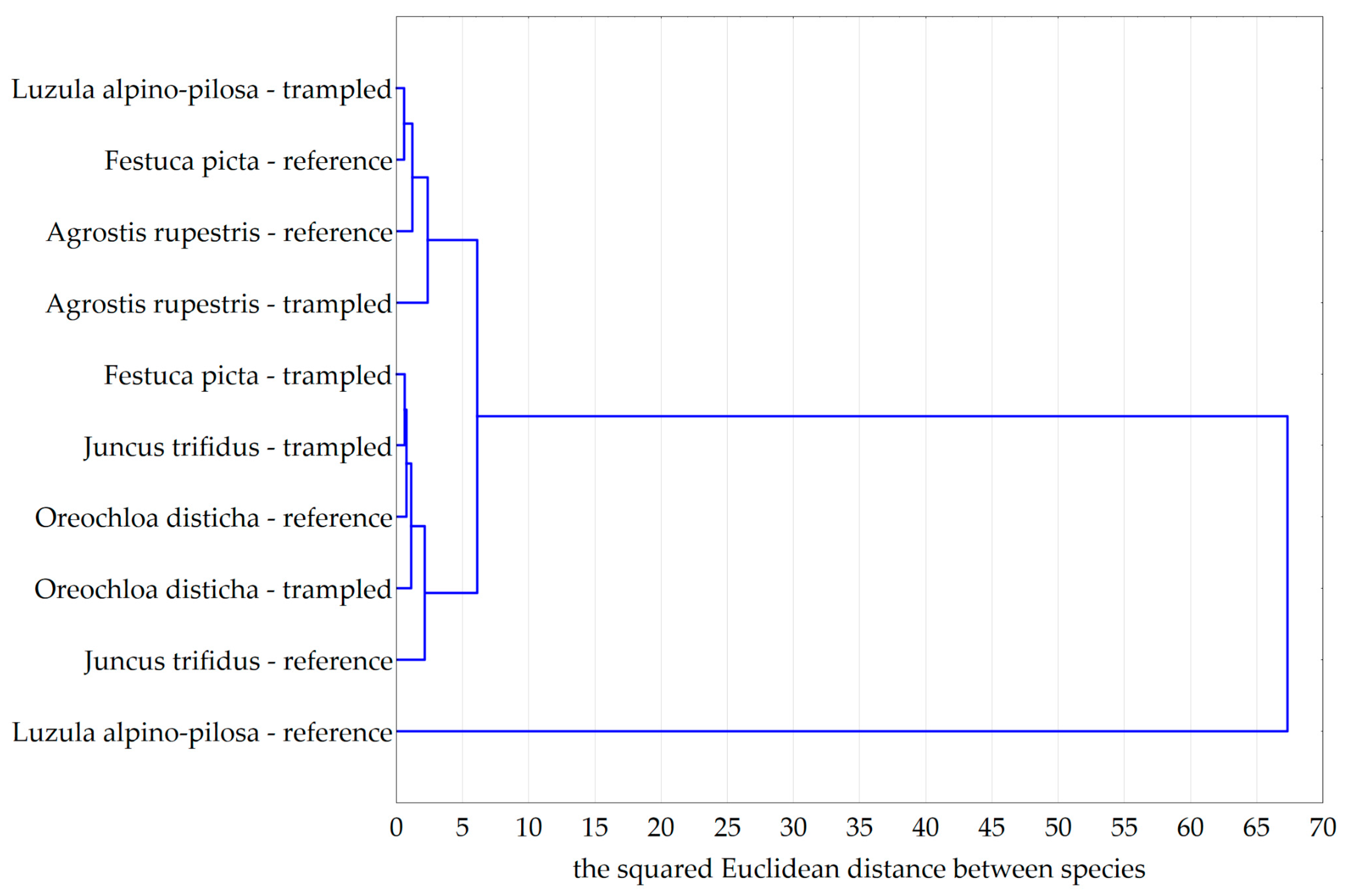
  • Plant Senescence Reflectance Index (PSRI) [55], Cellulose Absorption Index (CAI) [56];
  • Carotenoid Reflectance Index 1 (CRI 1) [57], Carotenoid Reflectance Index 2 (CRI2) [57], Anthocyanin Reflectance Index 1 (ARI 1) [58], and Anthocyanin Reflectance Index 2 (ARI 2) [58]; and
  • Moisture Stress Index (MSI) [59], Normalized Difference Infrared Index (NDII) [60], Water Band Index (WBI) [49], and Normalized Difference Water Index (NDWI) [61].
All statistical analyses were conducted on individual, single, measurements with graphs presented for average values. The first step was statistical analysis (Mann–Whitney U test, comparison of two groups-buffer up to 5 m, trampled and more than 5 m as a reference) of these remote sensing vegetation indices, to see which indices show statistically significant changes (level p < 0.05) in reaction to trampling compared to reference buffer measurements. The analysis of spectral reflection curves was also based on the Ward’s data agglomeration method. This method made it possible to compare the spectral characteristics of the dominant species of alpine swards, and to illustrate that the spectral reflectance curves of the species and their cases (trampled and reference) are most similar to each other in the values of reflectance in the range of 350–2500 nm. The characteristic result of this classification is a hierarchical tree, at the beginning of which each object is its own class. With each step, the criterion is weakened. In this way, more and more elements are related to each other more and more differently. In the last stage of the research, the objects are connected to each other. Then, in the cases of statistical significance (at the level p < 0.05), the parameters were analyzed using bio-radiometric measurements and fluorescence. For this purpose, the remote sensing vegetation indices (statistically significant at the p < 0.05 level) were correlated (using Spearman correlation because the data does not have a normal distribution) with bio-radiometric indices. This correlation was used to verify that the same information was obtained from the spectrometer measurements. Meanwhile, the Spearman correlation between remote sensing vegetation indices and measurements of fluorescence (Fv/Fm and t½) was used to verify that changes are genuinely caused by trampling and relate to cell disorders in the photosynthetic process.

4. Results

After analyzing the statistical tests, all the species studied and compare in both polygons showed statistically significant changes at the 0.05 level (Figure 4). This confirmation of a change, between trampled and reference vegetation, was visible in both the wavelength ranges corresponding to pigment concentration (especially chlorophyll), cellular structures (red edge), and the narrow ranges describing the water contents (Figure 4). All species had a common important range within the electromagnetic spectrum, and when looking for the signature of trampled vegetation. These ranges are related to the chlorophyll (621–693 nm), cell structure (1360–1372 and 1409–1529 nm) and water, dry matter content and plant building substances such as proteins and nitrogen (1829–1835, 1845–1862, 1879–2145, 2348–2465, and 2491–2500 nm; Table 2, Figure 4); additionally, uncovered soil causes increased transpiration and dryness of vegetation around the trail, as evidenced by the decrease in water content for the species in the buffer.
The effect of this research is to show differences in the condition of the examined species of alpine swards between test areas (trampled, reference) as well as interspecies variability. The agglomeration of the curves of spectral characteristics using the Ward method showed the degree of similarity of the spectral reflection value of individual species of alpine swards in the study field. The highest similarity of spectral characteristics was observed between polygon variants (trampled, reference) for the species Oreochloa disticha, Agrostis rupestris and Juncus trifidus. However, species Festuca picta and Luzula alpino-pilosa were significantly different from each other (trampled and reference) in the tested areas (Figure 5). If we compare only the dominant alpine swards species in reference polygons, the species with similar spectral characteristics are the species Festuca picta and Agrostis rupestris, as well as the second pair of similar species such as Oreochloa disticha and Juncus trifidus. However, the species that differs significantly from its spectral characteristics is Luzula alpino-pilosa (Figure 5).
To confirm the variation in stress status and variability of individual parameters (e.g., chlorophyll, and water content), the remote sensing indices were combined into groups that described specific features, i.e., condition and structure, chlorophyll content, nitrogen content, the amount of light used in the process of photosynthesis, and the water content. For the studied species, calculated values are significantly different (Table 3). The indicators that showed statistically significant differences between the reference and trampled polygons (at the statistical significance level of 0.05) for each species tested are SIPI, PSRI, MSI, NDII, WBI, NDWI, SAVI, WRDVI, SRPI, NDNI, and GI (Table 3). The remote sensing vegetation indices show a statistically significant decline in the value for trampled plants for all tested species. For example, the description of the general condition through Wide Dynamic Range Vegetation Index (WDRVI) decreased about 4–10% while the Soil-Adjusted Vegetation Index (SAVI) decreased by approximately 5–12%. There was also a decrease in chlorophyll content, e.g., SRPI decreases by approximately 3–31%, Greenness Index (GI) by 9–23% and Simple Ratio Pigment Index (SRPI) by 3–31%. The use of light in the photosynthesis process, detected using the Structure Insensitive Pigment Index (SIPI), decreased by approximately 3–7%. The nitrogen content (NDNI) varies between buffers by approximately 5–5.5% with the Plant Senescence Reflectance Index (PSRI) ranging 20–67%. The amount of water also decreased, as shown by NDWI, whose value for the trampled species decreased by approximately 50–100% alongside the Moisture Stress Index (MSI) by 11–22%, Normalized Difference Infrared Index (NDII) by 21–29% and Water Band Index (WBI) by 1–3%.
To verify the spectrometric measurements and the vegetation indices calculated on their basis, as well as to check conclusions concerning the degraded state of trampled plants, these values were correlated with bio-radiometric measurements; the results of bio-radiometric correlations for indices such as CCI, ts-ta and fAPAR (Table 4). The highest correlation was observed for chlorophyll content in the Agrostis rupestris and Luzula alpino-pilosa; these species have a wide leaf blade and bright green color, which visually indicates a much higher chlorophyll content. For the trampled species Agrostis rupestris, the chlorophyll value (CCI) correlates with GNDVI to the level of −0.67, indicating that the chlorophyll content has declined due to trampling. However, in the reference buffer, we observed a high relationship (0.71) between the chlorophyll content and GNDVI, which indicates that the amount of chlorophyll has not changed in the plant (Table 4). Overall, species correlation results from the spectrometer and bio-radiometric indices are different depending on the structure of the vegetation.
Analysing the community as a whole, a high correlation was observed between the ts-ta and NDWI or WBI—indices describing water in plants. In both the reference and trampled case, the ts-ta index for Oreochloa disticha was highly correlated with NDWI. However, for trampled plants it was −0.71, which means that the water content is lower than in the reference plant, where the correlation value is 0.49 meaning that the value of both indices increases. The highest correlation was observed for Juncus trifidus, in the trampled buffer, where the correlation between the index of ts-ta and WBI reached a value of −0.85; statistically significant at the 0.05 level (Table 4). With an increase in the observed water stress value of the ts-ta index, the value of the WBI decreased, confirming a decreasing water content in the trampled plants. Trampling also influences the use of light within photosynthesis, linking into the functioning of the plant, which has been verified by measurements of the amount of radiation used by photosynthesis. Thus, the fraction of the incoming solar radiation in the Photosynthetically Active Radiation spectral region that is absorbed by a photosynthetic organism, typically describing the light absorption across an integrated plant canopy (fAPAR) was calculated. The fAPAR index for Juncus trifidus in the trampled buffer zone correlated with the PRI (−0.39), which showed that the amount of light used in photosynthesis decreased through trampling (Table 4). NPQI correlated highly with fAPAR for trampled Luzula alpino-pilosa and Oreochloa disticha, which means that a lower chlorophyll, chlorophyll degradation (described by NPQI) is accompanied by a decrease in the use of light for photosynthesis. Both of these indicators (PRI and NPQI) belong to the group of indicators used to assess the amount of light used in photosynthesis.
To determine the actual cell status, caused by trampling, fluorescence measurements were undertaken. The Fv/Fm (with adaptation to darkness) value of fluorescence for trampled species was lowered by about 0.050–0.130 units (Table 5). Some species in the reference buffer had a higher value of Fv/Fm than the same species in the trampled buffer. For example, Luzula alpino-pilosa had an Fv/Fm value of 0.627 in the reference buffer and 0.596 for the trampled, which may indicate a lower efficiency of light absorption related to lower chlorophyll content (Table 5). For the three species Luzula alpino-pilosa, Agrostis rupestris, Festuca picta, the difference between the Fv/Fm value is statistically significant. For Luzula alpino-pilosa, it was also statistically significant (at the p < 0.05 level) compared with the difference between the reference and trampled plants as measured using Mann–Whitney U test. This means that the plant cells of this species are very sensitive to changes caused by trampling, and have a limited capacity for photosynthesis. The agglomeration of the curves was also confirmed by Ward’s method, where this species was the most differentiated between the trampled and reference polygon. The low values of Fv/Fm for leaves adapted to darkness may also be due to the plants’ growth in full sunlight slopes, which initiates the process of photoinhibition.
Generally, t½ (in ms) is a function of the photochemical reaction rate and pool size of electron acceptors, including the PQ pool; up to half the time it takes to reach maximum fluorescence. The difference for the investigated species, in the reference and trampled buffer, was low and not statistically significant at the 0.05 level that may indicate that plant cells functions are not disturbed. The observed morphological adaptation in previously studied species also confirmed their biochemical condition is due to their growth in the testing mountainous terrain, with leaf thickness and the number of layers of parenchyma contributing to the process of photosynthesis. To confirm this relationship, values obtained from the fluorometer were correlated to the indices illustrating the various vegetation parameters, such as cellular structures, pigments or water content. Overall, in the study, only those indices that revealed statistically significant differences at a 0.05 level were used.
Fv/Fm for the species Luzula alpino-pilosa in the reference buffer was strictly correlated with WBI (−0.67) that characterizes the water content, while Fv/Fm for the trampled Luzula alpino-pilosa correlates with REPI (0.36; Table 6). In addition, a high correlation is observed between Fv/Fm and GNDVI (Festuca picta), especially for trampled plants, which means that the plants were stressed; trampled plants have also a higher ratio of carotenoids to chlorophyll. The Juncus trifidus in the reference buffer shows the highest correlation with fluorescence indices representing the structure and condition of the plants (e.g., CAI), with values of −0.62, but for the trampled species Juncus trifidus the correlation value of Fv/Fm with GNDVI is −0.66, which means that these plants were stressed.
The fluorescence index (Fv/Fm) for the species Agrostis rupestris is in most cases positively correlated with remote sensing indices. For this species in the reference buffer, the Fv/Fm fluorescence value correlated with mNDVI705 indices (0.56), while, in the trampled buffer, the Fv/Fm correlated with TCARI indices (0.63). Plants under stress contain higher concentrations of carotenoids, which play a prominent role in protection against stress; this index is a measure of stressed vegetation. This is also reflected in photosynthesis and other processes that occur in a plant, as shown in Table 6, by the values of the fluorescence correlations (statistical significance at the level 0.05) between indices depicting chlorophyll (e.g., mNDVI705, REPI) or those describing the physiological state (e.g., GNDVI, TCARI) and indices determining the amount of light used in the process of photosynthesis (e.g., PRI), water content (e.g., WBI) or stress-related pigments SIPI and CAI (which determine the condition of trampling vegetation).
Trampling interacts in different ways with the studied species, which is visible via a changing reflectance spectrum and then remote sensing indicators. Changes caused by trampling mostly affect the spectral absorption bands related to pigments and water content. Moreover, the changes are also reflected in the values of Fv/Fm, which show different adaptation of the photosynthetic apparatus of each species.
Differences in the condition of species allow us to state clearly that the species are more or less resistant to trampling in this area. Luzula alpino-pilosa in the reference range differs most from the others, although together with the Juncus trifidus species belong to one family, their spectral characteristics are varied. Luzula alpino-pilosa also displays the largest statistically significant differences between the reference and trampled polygons. In addition, the remaining species in the reference polygons, presented in the studies, group in terms of spectral similarity into two groups. Looking at the species in reference polygons, we have the similarity of Festuca picta and Agrostis rupestris as well as Oreochloa disticha and Juncus trifidus. However, when it comes to differences between two types of polygons within the studied species, we can rank the tested species from those that showed the smallest differences to those that showed the greatest differences: Oreochloa disticha, Juncus trifidus, Agrostis rupestris, Festuca picta, and Luzula alpino-pilosa. Overall, all species threatened by trampling have a worse condition by about 10–30%, taking into account all the statistically significant analyzed indicators.

5. Discussion

Interspecific differences were most visible in the near-infrared range, which relates to cellular structures. Luzula alpino-pilosa and Festuca picta had the highest reflectances (about 0.80), while lower reflectances (of about 0.10–0.20) were measured for the remaining species tested. The largest differences between the species were in the spectral ranges describing chlorophyll content (621–693 nm), cellular structures (1360–1372 and 1409–1529 nm), and water content (1829–1835, 1845–1862, 1879–2145, 2348–2465, and 2491–2500 nm). The above ranges were also used by Ruban et al. [62], Gitelson et al. [58,59], Agapiou et al. [63] and et al. Fourty et al. [55] to evaluate vegetation changes. The most commonly used for water content and water stress are 950–970, 1150–1260, and 1520–1540 nm [47,64]. This type of analysis leads to the identification and grouping of species with similar characteristics, and hyperspectral imagery can be used to classify the species condition.
Hyperspectral research on the classification of highland grassland species in the Tatra National Park was initiated by Sobczak et al. [65] who measured spectral reflectance in the field, and Zagajewski [66] who classified hyperspectral airborne imagery. Sobczak [65] showed that spectral reflectance intraspecific differences for both Juncus trifidus and Luzula alpino-pilosa are linked to visual differences (e.g., leaf blade construction), and are an adaptation linked to excessive radiation (change in carotenoid to chlorophyll ratio). The greatest differences between species were in the range 500–650 nm, 700–1900 nm, and 2100–2450 nm [65]. In this article, the ranges are related to the chlorophyll (621–693 nm) and cell structure (1360–1372, 1409–1529 nm) alongside the water, dry matter content and plant building substances such as protein and nitrogen (1829–1835, 1845–1862, 1879–2145, 2348–2465, and 2491–2500 nm). Svalbard’ species are characterised by similar ranges; in this analysis, the most significant ranges were 446–506 nm (respectively, for the Polar plant species: 448–499 nm), 623–695 (Polar: 682–699 nm) and 1801–2500 (Polar: 1801–2399 nm) [67]. Even though the information obtained from the airborne (hyperspectral) images confirmed the dependence, interspecific differences were based on ground-based methods.
Zarco-Tejada et al. [68] conducted fieldwork on vineyards using hyperspectral data (CASI, ROSIS, DAIS-7915, terrestrial spectrometer) and bio-radiometric measurements (LAI). Estimates were made of chlorophyll a and b, carotenoids and the state of the vine. The authors determined that one of the best indications (R2 = 0.50) was the variability of the chlorophyll to carotenoid using the SIPI and PRI ratios, while the chlorophyll content is best correlated (R2 of around 0.80–0.90) with other vegetation indices such MCARI, TCARI, MCARI/OSAVI, and TCARI/OSAVI35 [67].
Kycko [35] noted that statistically significant changes in the spectral characteristics of species (significance level α = 0.05, α = 0.01, α = 0.001) were mainly represented in the spectral range of the plant pigments and water content. The bio-radiometric measurements, chlorophyll measurement (CCI) and fAPAR confirmed the information obtained from the spectrometer, with remote sensing indicators also used [32]. Kycko et al. [32] identified three groups of indicators (broadband greenness, narrowband greenness, and canopy water content groups) that were at a statistically significant level (α = 0.001) and represented changes over 70% for all the species measurements. The indicators for the given groups were: NDVI and ARVI; mSR705 and mNDVI705; WBI, NDWI and NDII; and ARVI, WBI and NDWI.
Overall, this study confirmed that vegetation condition may decline in response to many biotic and abiotic factors, e.g., alpine swards exposed to full sunlight, insufficient water supply and high temperatures alongside excessive tourist traffic. One of the stress factors is trampling, which leads to changes in some species, with remote sensing vegetation indices reflecting damaged structures and lower level of physiological processes.
The varied construction of each of the species studied and adaption to the area is reflected in the results of the spectrometry, bio-radiometry and fluorescence measurements. Changes caused by trampling are reflected in the vegetation’s status, lower spatial coverage, lower plant height, decreased biomass, changes in the typical species composition, relative changes in cover classes and displacement of species [69,70,71,72,73]. Cole [12] found that plant morphology was more significant than site characteristics (altitude, overstory canopy cover and total vegetation cover) in determining the response of vegetation to trampling. The same conclusion was reached by Sun and Liddle [74], who showed that plant height and morphological structure appear to be strongly associated with resistance to trampling. As a result, some alpine vegetation types may be significantly more resistant than sub-alpine and low-elevation types, due to the larger proportion of turf-forming graminoids [75,76]. However, Bell and Bliss [77] concluded that the other alpine vegetation types are less resistant, so studies show a diverse resistance to trampling amongst species. In this research, all species in the Czerwone Wierchy Peaks showed a statistically significant (p < 0.05) change between trampled and reference plants, which was visible in the reflectance spectrum curves.
However, vegetation can rebuild its structure and so in most cases (if trampling is not to a very high degree e.g., devastation of sites) recovery can occur, but alpine vegetation recovers much more slowly than vegetation in lower altitude areas [78,79]. The conducted research showed variable species resistance to trampling—a similar relationship to that shown by Dumitrascu [80], who emphasize that habitat characteristics affect the state of trampled plants. Species react differently to stress and this is dependent on their morphology, anatomy and state of development at any given moment. In Dumitrascu [80] changes were observed in the chlorophyll concentration within the leaves, revealing, respectively, a decrease or increase in the visible range reflectance around 700 nm [81]. A similar situation can be seen in this study, where the stress caused by excessive trampling is visible in the same wavelength range indicating chlorophyll, as evidenced by the remote sensing of vegetation indicators such as SRPI, that the difference between trampled and reference plants is about 0.10–0.20. Moreover, these changes are statistically significant at the p < 0.05 level for all species studied [82].
When plants are exposed to abiotic and biotic stress in high light conditions, decreases in Fv/Fm are frequently observed [83]. The optimum range is 0.79–0.84, but this varies [84]; a lower value is seen when the plant has been exposed to stress, indicating photoinhibition [85]. The Fv/Fm parameter appears to be relatively insensitive to severe water limitation but could be used to differentiate between responses at cold temperatures. High light intensity is observed in the mountains, thus Fv/Fm values obtained in this study range between 0.471 and 0.627. Kalaji [28] observed that heat stress significantly prolonged the time to achieve maximum fluorescence (TFM)—190% compared to controls—and increased the reduction of QA from 0 to TFM (N) by 230% compared to control plants. In the present study, a decrease in half-time (t½) between the trampling and the reference plant was not observed [86], which may suggest that, despite the small difference in Fv/Fm values, reaction centers are not disrupted and photochemical processes in the studied plant species work well. Therefore, we can conclude that temperature is not an important stress factor for alpine swards, where plants are well adapted to adverse environmental conditions [87]. Literature data suggest that most of the stresses affecting the photosynthetic apparatus reduce the Fv/Fm ratio, while some authors suggest constant values are measured during drought conditions [88,89,90].
The high correlation index of Fv/Fm with indicators from the group describing the use of light within the photosynthetic process (PRI, NPQI) allows for long-term monitoring of vegetation. One example is the research of Tan et al. [91] where, when determining damage to corn, the SIPI index was used and was highly correlated to Fv/Fm (R = 0.88). In this study, the SIPI correlated highly with Fv/Fm (R = 0.77) for Oreochloa disticha and PRI correlated with Fv/Fm (R = 0.54) for Festuca picta indicating changes in the reference vegetation that included higher energy consumption. GNDVI, defined as a modification and improvement of the NDVI index for highlighting the physiological properties of plants [92], showed a high correlation with CCI, e.g., for Agrists rupestris is was 0.71, which showed good development in the reference vegetation compared to the disturbed state of trampled vegetation. Fv/Fm had a high correlation with the indices, indicating the amount of chlorophyll and use of light for photosynthesis. For example, for the reference samples of Oreochloa disticha, the Fv/Fm ratio correlates at 0.77 with the SIPI index, while for the same species threatened by trampling, we have the opposite (negative) correlation. The best vegetation indices, which were statistically significant for the analyses, were NDVI, mNDVI, NDVI705, mSR705, ARVI, EVI, WBI, NDWI and NDII.
Replanting of the vegetation is possible, although very labor intensive [93]. In addition, the impact of informal trails can be particularly problematic, because subalpine and alpine plant communities on mountain summits are typically fragile, spatially restricted and rare [94,95]. Therefore, through the analysis of the vegetation state and information about fluorescence, we are able to closely monitor and evaluate plant species exposed to environmental stress before external signals (yellowing or browning of leaves) are visible. Such monitoring of vegetation state allows earlier prevention of the destruction of a species in valuable natural areas such as, amongst others, national parks [96,97].

6. Conclusions

High grassland dominant species, such as alpine vegetation, are characterized by a set of unique properties that can be measured with hyperspectral sensors and confirmed by fluorescence measurements. The most important are plant pigments (including their relative concentrations), protective elements, e.g., the shape and structure of leaves, or waxy cover. The analysis captured the impact of both biotic and abiotic factors on the species, thus reflecting the actual condition of the vegetation. Trampling disintegrates the plant canopy, causing higher transmission of solar radiation and changes in water-temperature relationships (increases in soil temperature and transpiration). Therefore, it is valuable to monitor plant condition, especially in areas often visited by tourists.
The applied methods, which combine spectral characteristics and vegetation indices containing information on fluorescence, allow for a detailed analysis. The hyperspectral measurements confirmed statistically significant differences between trampled and reference plants. The changes were observed in chlorophyll absorption, cell structures and water content; the observations were confirmed by chlorophyll content, fluorescence and the ts-ta temperature index. The fluorescence ratio (Fv/Fm) was used to evaluate the efficiency of chlorophyll in the photosynthetic process. The use of statistical correlation allowed the impact of heavy tourist traffic on the selected species to be determined, including the variable response; important for the protection of valuable natural areas. It is possible to determine which species exhibited the largest/smallest indicator variation, which, ranked from smallest to largest, are Oreochloa disticha, Juncus trifidus, Agrostis rupestris, Festuca picta, and Luzula alpino-pilosa. The largest percentage of variation detected for Luzula alpino-pilosa is related to the broad leaf blades of the plant, their thickness and size. On the other hand, Oreochlo disticha has harder leaves and stems, which translates into a lower percentage (52%) of change caused by trampling. Therefore, the morphology and physiology of plants is important not only for their adaptation to living in the mountainous terrain but also for the impact of trampling. The use of hyperspectral data confirms the rich information available for vegetation state, especially vegetation endangered by trampling, but also confirms fluorescence measurements as an indicator for describing the actual state of the pigments and cell structures.
With the rapid development of remote sensing technology, newer remote and non-invasive methods for measuring chlorophyll fluorescence are being developed; for example, the Fluorescence Explorer (FLEX) satellite mission due to launch in 2022. However, FLEX is planned to have a spatial resolution of 300 m, which is insufficient for biodiversity testing and assessment of species condition, but can be useful for analyzing larger plant communities or preserving whole areas of the landscape. Hyperspectral analysis, using airborne or UAV data, seems to be more appropriate for smaller areas.

Acknowledgments

Authors would like to thank the Tatra National Park, Institute of Geography and Spatial Organisation of Polish Academy of Sciences and the Anna Pasek Foundation, which in 2012/2013 funded a scholarship to Marlena Kycko. The method of field data acquisition was developed in the frame of the Polish–Norwegian Research Programme, National Centre for Research and Development project: Ecosystem stress from the combined effects of winter climate change and air pollution—how do the impacts differ between biomes? (WICLAP), No.: POL-NOR/198571/83/2013 and the Biostrateg Programme of the Polish National Centre for Research and Development (NCBiR), project No. DZP/BIOSTRATEG-II/390/2015: The innovative approach supporting monitoring of non-forest Natura 2000 habitats, using remote sensing methods (HabitARS), and the publishing costs were financed from grants for science awarded by the Polish Ministry of Science and Higher Education under the theme No. 501-D119-64-0180200-15. Special thanks also go to students participating in the study: Aneta Modzelewska, Olga Kurek, and Ignacy Kaźmierczak, as well as the Tatra National Park Volunteers Adam Lubiński and Michał Kozioł.

Author Contributions

Bogdan Zagajewski and Marlena Kycko conceived and designed the experiment; Marlena Kycko, Bogdan Zagajewski, Elżbieta Romanowska and Magdalena Zwijacz-Kozica performed the field measurements and analyzed the acquired data, and all authors wrote the paper.

Conflicts of Interest

The authors declare no conflict of interest.

References

  1. Gamon, J.A.; Field, C.B.; Roberts, D.A.; Ustin, S.L.; Valentini, R. Functional patterns in an annual grassland during an AVIRIS overflight. Remote Sens. Environ. 1993, 44, 239–253. [Google Scholar] [CrossRef]
  2. Roberts, D.A.; Batista, G.T.; Pereira, J.; Waller, E.K.; Nelson, B.W. Change identification using multitemporal spectral mixture analysis: Applications in Eastern Amazonia. In Remote Sensing Change Detection: Environmental Monitoring Applications and Methods; Elvidge, C., Lunetta, R., Eds.; Ann Arbor Press: Chelsea, MI, USA, 1998; pp. 137–161. [Google Scholar]
  3. Kupková, L.; Červená, L.; Suchá, R.; Jakešová, L.; Zagajewski, B.; Březina, S.; Albrechtová, J. Classification of Tundra Vegetation in the Krkonoše Mts. National Park Using APEX, AISA Dual and Sentinel-2A Data. Eur. J. Remote Sens. 2017, 50, 29–46. [Google Scholar] [CrossRef]
  4. Raczko, E.; Zagajewski, B.; Ochtyra, A.; Jarocińska, A.; Marcinkowska-Ochtyra, A.; Dobrowolski, M. Forest species identification of Mount Chojnik (Karkonoski National Park) using airborne hyperspectal APEX data. Sylwan 2015, 159, 593–599. [Google Scholar]
  5. Raczko, E.; Zagajewski, B. Comparison of Support Vector Machine, Random Forest and Neural Network Classifiers for Tree Species Classification on Airborne Hyperspectral APEX images. Eur. J. Remote Sens. 2017, 50, 144–154. [Google Scholar] [CrossRef]
  6. Tucker, C.J.; Sellers, P.J. Satellite remote sensing of primary production. Int. J. Remote Sens. 1986, 7, 1395–1416. [Google Scholar] [CrossRef]
  7. Knipling, E.B. Physical and physiological basis for the reflectance of visible and near-infrared radiation from vegetation. Remote Sens. Environ. 1970, 1, 155–159. [Google Scholar] [CrossRef]
  8. Whinam, J.; Chilcott, N.M. Impact after four years of experimental trampling on alpine/sub-alpine environments in western Tasmania. J. Environ. Manag. 2003, 67, 339–351. [Google Scholar] [CrossRef]
  9. Cierniewski, J.; Kazmierowski, C.; Krolewicz, S.; Piekarczyk, J.; Wrobel, M.; Zagajewski, B. Effects of Different Illumination and Observation Techniques of Cultivated Soils on Their Hyperspectral Bidirectional Measurements under Field and Laboratory Conditions. IEEE J. Sel. Top. Appl. Earth Obs. Remote Sens. 2014, 7, 2525–2530. [Google Scholar] [CrossRef]
  10. Cierniewski, J.; Ceglarek, J.; Karnieli, A.; Królewicz, S.; Kaźmierowski, C.; Zagajewski, B. Predicting the diurnal blue-sky albedo of soils using their laboratory reflectance spectra and roughness indices. J. Quant. Spectrosc. Radiat. Transf. 2017, 200, 25–31. [Google Scholar] [CrossRef]
  11. Cole, D.N. Experimental trampling of vegetation. I. Relationship between trampling intensity and vegetation response. J. Appl. Ecol. 1995, 32, 203–214. [Google Scholar] [CrossRef]
  12. Cole, D.N. Experimental trampling of vegetation. II. Prediction of resistance and resilience. J. App. Ecol. 1995, 32, 215–224. [Google Scholar] [CrossRef]
  13. Cole, D.N.; Bayfield, N.G. Recreational trampling of vegetation: Standard experimental procedures. Biol. Conserv. 1993, 63, 209–215. [Google Scholar] [CrossRef]
  14. Gremmen, N.J.M.; Smith, V.R.; van Tongeren, O.F.R. Impact of trampling on the vegetation of subantarctic Marion Island. Arct. Antarct. Alp. Res. 2003, 35, 442–446. [Google Scholar] [CrossRef]
  15. Jägerbrand, A.K.; Alatalo, J.M. Effects of human trampling on abundance and diversity of vascular plants, bryophytes and lichens in alpine heath vegetation, Northern Sweden. SpringerPlus 2015, 4, 95. [Google Scholar] [CrossRef] [PubMed]
  16. McDougall, K.L.; Wright, G.T. The impact of trampling on feldmark vegetation in Kosciuszko National Park, Australia. Aust. J. Bot. 2004, 52, 315–320. [Google Scholar] [CrossRef]
  17. Barros, A.; Gonnet, J.; Pickering, C. Impacts of informal trails on vegetation and soils in the highest protected area in the Southern Hemisphere. J. Environ. Manag. 2013, 127, 50–60. [Google Scholar] [CrossRef] [PubMed]
  18. Ballantyne, M.; Pickering, C.M.; McDougall, K.L.; Wright, G.T. Sustained impacts of a hiking trail on changing windswept feldmark vegetation in the Australian Alps. Aust. J. Bot. 2014, 62, 263–275. [Google Scholar] [CrossRef]
  19. Kobayashi, Y.; Kaya, H.; Goto, K.; Iwabuchi, M.; Araki, T. A pair of related genes with antagonistic roles in mediating flowering signals. Science 1999, 286, 1960–1962. [Google Scholar] [CrossRef] [PubMed]
  20. Cole, D.N.; Monz, C.A. Trampling Disturbance of High-Elevation Vegetation, Wind River Mountains, Wyoming, U.S.A. Arct. Antarct. Alp. Res. 2002, 34, 365–376. [Google Scholar] [CrossRef]
  21. Sunohara, Y.; Ikeda, H.; Tsukgashi, S.; Murata, Y.; Sakurai, N.; Noma, Y. Effects of trampling on morphology and ethylene production in asiatic plantain. Weed Sci. 2002, 50, 479–484. [Google Scholar] [CrossRef]
  22. Sunohara, Y.; Ikeda, H. Effects of trampling and ethephon on leaf morphology in trampling-tolerant Plantago asiatica and Eleusine indica. Weed Res. 2003, 43, 155–162. [Google Scholar] [CrossRef]
  23. Striker, G.G.; Mollard, F.P.O.; Grimoldi, A.A.; Leon, R.J.C.; Insausti, P. Trampling enhances the dominance of graminoids over forbs in flooded grassland mesocosms. Appl. Veg. Sci. 2010, 14, 95–106. [Google Scholar] [CrossRef]
  24. Klug, B.; Scharfetter-Lehrl, G.; Scharfetter, E. Effects of trampling on vegetation above the timberline in the eastern Alps, Austria. Arct. Antarct. Alp. Res. 2002, 34, 377–388. [Google Scholar] [CrossRef]
  25. Scott, J.J.; Kirkpatrick, J.B. Effects of human trampling on the sub-Antarctic vegetation of Macquarie Island. Polar Rec. 1994, 30, 207–220. [Google Scholar] [CrossRef]
  26. Hortensteiner, S. Chlorophyll degradation during senescence. Annu. Rev. Plant Biol. 2006, 57, 55–77. [Google Scholar] [CrossRef] [PubMed]
  27. Tsimilli-Michael, M.; Strasser, R.J. In vivo assessment of plants’ vitality: Applications in detecting and evaluating the impact of mycorrhization on host plants. In Mycorrhiza: State of the Art, Genetics and Molecular Biology, Eco-Function, Biotechnology, Eco-Physiology, Structure and Systematics, 3rd ed.; Varma, A., Ed.; Springer: Berlin/Heidelberg, Germany, 2008; pp. 679–703. [Google Scholar] [CrossRef]
  28. Kalaji, M.H.; Bosa, K.; Kościelniak, J.; Hossain, Z. Chlorophyll a fluorescence—A useful tool for the early detection of temperature stress in spring barley (Hordeum vulgare L.). OMICS 2011, 15, 925–934. [Google Scholar] [CrossRef] [PubMed]
  29. Kalaji, M.H.; Guo, P. Chlorophyll fluorescence: A useful tool in barley plant breeding programs. In Photochemistry Research Progress; Sanchez, A., Gutierrez, S.J., Eds.; Nova Publishers: New York, NY, USA, 2008; pp. 439–463. [Google Scholar]
  30. Sharma, D.K.; Andersen, S.B.; Ottosen, C.O.; Rosenqvist, E. Wheat cultivars selected for high Fv/Fm under heat stress maintain high photosynthesis, total chlorophyll, stomatal conductance, transpiration and dry matter. Physiol. Plant. 2015, 153, 284–298. [Google Scholar] [CrossRef] [PubMed]
  31. Kycko, M.; Zagajewski, B.; Zwijacz-Kozica, M.; Cierniewski, J.; Romanowska, E.; Orłowska, K.; Ochtyra, A.; Jarocińska, A. Assessment of Hyperspectral Remote Sensing for Analyzing the Impact of Human Trampling on Alpine Swards. Mt. Res. Dev. 2017, 37, 66–74. [Google Scholar] [CrossRef]
  32. Zagajewski, B.; Jarocinska, A. Analysis of plant condition of the Bystrzanka catchment. In Remote Sensing for a Changing Europe, Proceedings of the 28th EARSeL Symposium, Istanbul, Turkey, 2–5 June 2008; Maktav, D., Ed.; IOS Press: Amsterdam, The Netherlands, 2009; pp. 498–504. [Google Scholar] [CrossRef]
  33. Bareth, G.; Aasen, H.; Bendig, J.; Gnyp, M.L.; Bolten, A.; Jung, A.; Michels, R.; Soukkamäki, J. Low-weight and UAV-based Hyperspectral Full-frame Cameras for Monitoring Crops: Spectral Comparison with Portable Spectroradiometer Measurements. Photogramm. Fernerkund. Geoinf. 2015, 1, 69–79. [Google Scholar] [CrossRef]
  34. Kycko, M.; Zagajewski, B.; Kozłowska, A. Variability in spectral characteristics of trampled high-mountain grasslands. Misc. Geogr. 2014, 18, 10–14. [Google Scholar] [CrossRef]
  35. Kozłowska, A.; Rączkowska, Z.; Zagajewski, B. Links between vegetation and morphodynamics of high-mountain slopes in the Tatra Mountain. Geogr. Pol. 2006, 79, 27–39. [Google Scholar]
  36. Pitman, J.I. Absorption of Photosynthetically Active Radiation, Radiation Use Efficiency and Spectral Reflectance of Bracken [Pteridium aquilinum (L.) Kuhnl] Canopies. Ann. Bot. 2000, 85 (Suppl. B), 101–111. [Google Scholar] [CrossRef]
  37. Kozłowska, A. Detailed mapping of high vegetation in the Tatra Mts. Pol. Bot. Stud. 2006, 22, 333–341. [Google Scholar]
  38. Björkman, O.; Demmig, B. Photon yield of O2 evolution and chlorophyll fluorescence characteristics at 77 K among vascular plants of diverse origins. Planta 1987, 170, 489–504. [Google Scholar] [CrossRef] [PubMed]
  39. Johnson, G.N.; Young, A.J.; Scholes, J.D.; Horton, P. The dissipation of excess excitation energy in British plant species. Plant Cell Environ. 1993, 16, 673–679. [Google Scholar] [CrossRef]
  40. Jarocińska, A.M.; Kacprzyk, M.; Marcinkowska-Ochtyra, A.; Ochtyra, A.; Zagajewski, B.; Meuleman, K. The application of APEX images in the assessment of the state of non-forest vegetation in the Karkonosze Mountains. Misc. Geogr. 2016, 20, 21–27. [Google Scholar] [CrossRef]
  41. Gitelson, A.A. Wide Dynamic Range Vegetation Index for Remote Quantification of Biophysical Characteristics of Vegetation. J. Plant Physiol. 2004, 161, 165–173. [Google Scholar] [CrossRef] [PubMed]
  42. Huete, A. A Soil-Adjusted Vegetation Index (SAVI). Remote Sens. Environ. 1988, 25, 295–309. [Google Scholar] [CrossRef]
  43. Gitelson, A.A.; Kaufman, Y.J.; Merzlyak, M.N. Use of a green channel in remote sensing of global vegetation from EOS-MODIS. Remote Sens. Environ. 1996, 58, 289–298. [Google Scholar] [CrossRef]
  44. Zarco-Tejada, P.J.; Bejron, A.; Miller, J.R. Stress Detection in Crops with Hyperspectral Remote Sensing and Physical Simulation Models. In Proceedings of the Airborne Imaging Spectroscopy Workshop, Bruges, Belgium, 8 October 2004. [Google Scholar]
  45. Dawson, T.P.; Curran, P.J. Technical note: A new technique for interpolating the reflectance red edge position. Int. J. Remote Sens. 1998, 11, 2133–2139. [Google Scholar] [CrossRef]
  46. Sims, D.A.; Gamon, J.A. Relationships Between Leaf Pigment Content and Spectral Reflectance Across a Wide Range of Species, Leaf Structures and Developmental Stages. Remote Sens. Environ. 2002, 81, 337–354. [Google Scholar] [CrossRef]
  47. Haboudane, D.; Miller, J.R.; Pattey, E.; Zarco-Tejada, P.J.; Strachan, I.B. Hyperspectral Vegetation Indices and Novel Algorithms for Predicting Green LAI of Crop Canopies: Modeling and Validation in the Context of Precision Agriculture. Remote Sens. Environ. 2004, 90, 337–352. [Google Scholar] [CrossRef]
  48. Daughtry, C.; Walthall, C.L.; Kim, M.S.; Brown de Colstoun, E.; McMurtreym, J.E. Estimating Corn Leaf Chlorophyll Concentration from Leaf and Canopy Reflectance. Remote Sens. Environ. 2000, 74, 229–239. [Google Scholar] [CrossRef]
  49. Peñuelas, J.; Gamon, J.A.; Fredeen, A.L.; Merino, J.; Field, C.B. Reflectance Indices Associated with Physiological Changes in Nitrogen and Water Limited Sunflower Leaves. Remote Sens. Environ. 1994, 48, 135–146. [Google Scholar] [CrossRef]
  50. Peñuelas, J.; Baret, F.; Filella, I. Semi-Empirical Indices to Assess Carotenoids/Chlorophyll—A Ratio from Leaf Spectral Reflectance. Photosynthetica 1995, 31, 221–230. [Google Scholar]
  51. Barnes, J.D.; Balaguer, L.; Manrique, E.; Elvira, S.; Davison, A.W. A reappraisal of the use of DMSO for the extraction and determination of chlorophylls a and b in lichens and higher plants. Environ. Exp. Bot. 1992, 32, 85–100. [Google Scholar] [CrossRef]
  52. Gamon, J.A.; Penuelas, J.; Field, C.B. A Narrow-Waveband Spectral Index That Tracks Diurnal Changes in Photosynthetic Efficiency. Remote Sens. Environ. 1992, 41, 35–44. [Google Scholar] [CrossRef]
  53. Gamon, J.A.; Field, C.B.; Bilger, W.; Bjorkman, O.; Fredeen, A.L.; Peñuelas, J. Remote sensing of xanthophyll cycle and chlorophyll fluorescence in sunflower leaves and canopies. Oecologia 1990, 85, 1–7. [Google Scholar] [CrossRef] [PubMed]
  54. Fourty, T.; Baret, F.; Jacquemoud, S.; Schmuck, G.; Verdebout, J. Leaf Optical Properties with Explicit Description of Its Biochemical Composition. Direct and Inverse Problems. Remote Sens. Environ. 1996, 56, 104–117. [Google Scholar] [CrossRef]
  55. Merzlyak, J.R.; Gitelson, A.A.; Chivkunova, O.B.; Rakitin, V.Y. Non-destructive Optical Detection of Pigment Changes During Leaf Senescence and Fruit Ripening. Physiol. Plant. 1999, 106, 135–141. [Google Scholar] [CrossRef]
  56. Nagler, P.L.; Inoue, Y.; Glenn, E.P.; Russ, A.L.; Daughtry, C.S.T. Cellulose absorption index (CAI) to quantify mixed soil–plant litter scenes. Remote Sens. Environ. 2003, 87, 310–325. [Google Scholar] [CrossRef]
  57. Gitelson, A.A.; Zur, Y.; Chivkunova, O.B.; Merzlyak, M.N. Assessing carotenoid content in plant leaves with reflectance spectroscopy. Photochem. Photobiol. 2002, 75, 272–281. [Google Scholar] [CrossRef]
  58. Gitelson, A.A.; Merzylak, M.N.; Chivkunowam, O.B. Optical properties and nondestructive estimation of anthocyanin content in plant leaves. Photochem. Photobiol. 2001, 74, 38–45. [Google Scholar] [CrossRef]
  59. Rock, B.N.; Williams, D.L.; Vogehnann, J.E. Field and airborne spectral characterization of suspected acid deposition damage in red spruce (Picea rubens) form Vermont. In Proceedings of the 11th International Symposium Machine Processing of Remotely Sensed Data, Lafayette, IN, USA, 25–27 June 1985; pp. 71–81. [Google Scholar]
  60. Hardisky, M.A.; Klemas, V.; Smart, R.M. The Influences of Soil Salinity, Growth Form, and Leaf Moisture on the Spectral Reflectance of Spartina Alterniflora Canopies. Photogramm. Eng. Remote Sens. 1983, 49, 77–83. [Google Scholar]
  61. Gao, B.C. NDWI—A normalized difference water index for remote sensing of vegetation liquid water from space. Remote Sens. Environ. 1996, 58, 257–266. [Google Scholar] [CrossRef]
  62. Ruban, A.V.; Young, A.J.; Horton, P. Induction of Nonphotochemical Energy Dissipation and Absorbance Changes in Leaves (Evidence for Changes in the State of the Light-Harvesting System of Photosystem II In Vivo). Plant Physiol. 1993, 102, 741–750. [Google Scholar] [CrossRef] [PubMed]
  63. Agapiou, A.; Hadjimitsis, D.G.; Alexakis, D.D. Evaluation of Broadband and Narrowband Vegetation Indices for the Identification of Archaeological Crop Marks. Remote Sens. 2012, 4, 3892–3919. [Google Scholar] [CrossRef]
  64. Rodriguez-Perez, J.R.; Riano, D.; Carlisle, E.; Ustin, S.; Smart, D.R. Evaluation of hyperspectral reflectance indices to detect grapevine water status in vineyard. Am. J. Enol. Vitic. 2007, 58, 302–317. [Google Scholar]
  65. Sobczak, M.; Folbrier, A.; Kozłowska, A.; Krówczyńska, M.; Pabjanek, P.; Wrzesień, M.; Zagajewski, B. Assessment of the potential of hyperspectral data and techniques for mountain vegetation analysis. In Imaging Spectroscopy. New Quality in Environmental Studies; Zagajewski, B., Sobczak, M., Eds.; EARSeL & Warsaw University, Faculty of Geography and Regional Studies: Warsaw, Poland, 2005; pp. 761–780. [Google Scholar]
  66. Zagajewski, B. Assessment of neural networks and Imaging Spectroscopy for vegetation classification of the High Tatras. Teledetekcja Środowiska 2010, 43, 113. [Google Scholar]
  67. Zagajewski, B.; Tømmervik, H.; Bjerke, J.W.; Raczko, E.; Bochenek, Z.; Kłos, A.; Jarocińska, A.; Lavender, S.; Ziółkowski, D. Intraspecific Differences in Spectral Reflectance Curves as Indicators of Reduced Vitality in High-Arctic Plants. Remote Sens. 2017, 9, 1289. [Google Scholar] [CrossRef]
  68. Zarco-Tejada, P.J.; Berjón, A.; López-Lozano, R.; Miller, J.R.; Martín, P.; Cachorro, V.; González, M.R.; de Frutos, A. Assessing vineyard condition with hyperspectral indices: Leaf and canopy reflectance simulation in a row-structured discontinuous canopy. Remote Sens. Environ. 2005, 99, 271–287. [Google Scholar] [CrossRef]
  69. Marcinkowska-Ochtyra, A.; Zagajewski, B.; Ochtyra, A.; Jarocińska, A.; Wojtuń, B.; Rogass, C.; Mielke, C.; Lavender, S. Subalpine and alpine vegetation classification based on hyperspectral APEX and simulated EnMAP images. Int. J. Remote Sens. 2017, 38, 1839–1864. [Google Scholar] [CrossRef]
  70. Liddle, M.J. A theoretical relationship between the primary productivity of vegetation and its ability to tolerate trampling. Biol. Conserv. 1975, 8, 251–255. [Google Scholar] [CrossRef]
  71. Liddle, M.J. Recreation Ecology: The Ecological Impact of Outdoor Recreation and Ecotourism; Chapman & Hall: London, UK, 1997; p. 639. [Google Scholar]
  72. Cole, D.N.; Spildie, D.R. Hiker, horse and llama trampling effects on native vegetation in Montana, USA. J. Environ. Manag. 1998, 53, 61–71. [Google Scholar] [CrossRef]
  73. Littlemore, J.; Barker, S. The ecological response of forest ground flora and soils to experimental trampling in British urban woodlands. Urban Ecosyst. 2001, 5, 257–276. [Google Scholar] [CrossRef]
  74. Sun, D.; Liddle, M.J. Plant morphological characteristics and resistance to simulated trampling. Environ. Manag. 1993, 17, 511–521. [Google Scholar] [CrossRef]
  75. Price, M.F. Impacts of recreational activities on alpine vegetation in western North America. Mt. Res. Dev. 1985, 5, 263–277. [Google Scholar] [CrossRef]
  76. Monz, C.A. The response of two arctic tundra plant communities to human trampling disturbance. J. Environ. Manag. 2002, 64, 207–217. [Google Scholar] [CrossRef]
  77. Bell, K.L.; Bliss, L.C. Alpine disturbance studies: Olympic National Park USA. Biol. Conserv. 1973, 5, 25–32. [Google Scholar] [CrossRef]
  78. Calais, S.S.; Kirkpatrick, J.B. Impact of Trampling on Natural Ecosystems in the Cradle Mountain-Lake St Clair National Park. Aust. Geogr. 1986, 17, 6–15. [Google Scholar] [CrossRef]
  79. Bjerke, J.W.; Karlsen, S.R.; Høgda, K.A.; Malnes, E.; Jepsen, J.U.; Lovibond, S.; Vikhamar Schuler, D.; Tømmervik, H. Record-low primary productivity and high plant damage in the Nordic Arctic Region in 2012 caused by multiple weather events and pest outbreaks. Environ. Res. Lett. 2014, 9, 084006. [Google Scholar] [CrossRef]
  80. Dumitrascu, M.; Marin, A.; Preda, E.; Tibirnac, M.; Vadineanu, A. Trampling effects on plant species morphology. Rom. J. Biol. Plant Biol. 2010, 55, 89–96. [Google Scholar]
  81. Carter, G.A.; Knapp, A.K. Leaf optical properties in higher plants: Linking spectral characteristics to stress and chlorophyll concentration. Am. J. Bot. 2001, 88, 677–684. [Google Scholar] [CrossRef] [PubMed]
  82. Broge, N.; Leblanc, E. Comparing Prediction Power and Stability of Broadband and Hyperspectral Vegetation Indices for Estimation of Green Leaf Area and Canopy Chlorophyll Density. Remote Sens. Environ. 2000, 76, 156–172. [Google Scholar] [CrossRef]
  83. Baker, N.R. Chlorophyll fluorescence: A probe of photosynthesis in vivo. Annu. Rev. Plant Biol. 2008, 59, 89–113. [Google Scholar] [CrossRef] [PubMed]
  84. Bolhàr-Nordenkampf, H.R.; Öquist, G.O. Chlorophyll fluorescence as a tool in photosynthesis research. In Photosynthesis and Production in a Changing Environment. A Field and Laboratory Manual; Hall, D.O., Scurlock, J.M.O., Bolhàr-Nordenkampf, H.R., Leegoood, R.C., Long, S.P., Eds.; Chapman & Hall: London, UK, 1993; pp. 193–206. [Google Scholar] [CrossRef]
  85. Maxwell, K.; Johnson, G.N. Chlorophyll fluorescence—A practical guide. J. Exp. Bot. 2000, 51, 659–668. [Google Scholar] [CrossRef] [PubMed]
  86. Strasser, R.J.; Srivastava, A.; Tsimilli-Michael, M. The fluorescence transient as a tool to characterize and screen photosynthetic samples. In Probing Photosynthesis: Mechanism, Regulation and Adaptation; Yunus, M., Pathre, U., Mohanty, P., Eds.; Taylor and Francis: London, UK, 2000; pp. 443–480. [Google Scholar]
  87. Gola Golan, T.; Li, X.P.; Müller-Moulé, P.; Niyogi, K.K. Using mutants to understand light stress acclimationin plants. In Chlorophyll Fluorescence: A Signature of Photosynthesis; Papageorgiou, G.C., Ed.; Springer: Dordrecht, The Netherlands, 2004; pp. 525–554. [Google Scholar]
  88. Kaiser, W.M. Effect of water deficit on photosynthetic capacity. Physiol. Plant. 1987, 71, 142–149. [Google Scholar] [CrossRef]
  89. Ohashi, Y.; Nakayama, N.; Saneoka, H.; Fujita, K. Effects of drought stress on photosynthetic gas exchange, chlorophyll fluorescence and stem diameter of soybean plants. Biol. Plant. 2006, 50, 138–141. [Google Scholar] [CrossRef]
  90. Guóth, A.; Tari, I.; Gallé, A.; Csiszár, J.; Horváth, F.; Pécsváradi, A.; Cseuz, L.; Erdei, L. Chlorophyll a fluorescence induction parameters of flag leaves characterize genotypes and not the drought tolerance of wheat during grain filling under water deficit. Acta Biol. Szeged. 2009, 53, 1–7. [Google Scholar]
  91. Tan, C.W.; Huang, W.J.; Jin, X.L.; Wang, J.C.; Tong, L.; Wang, J.H.; Guo, W.S. Monitoring the chlorophyll fluorescence parameter Fv/Fm in compact corn based on different hyperspectral vegetation indices. Spectrosc. Spectr. Anal. 2012, 32, 1287–1291. [Google Scholar]
  92. Gitelson, A.A.; Merzlyak, M.N. Spectral Reflectance Changes Associated with Autumn Senescence of Aesculus hippocastanum L. and Acer platanoides L. Leaves. Spectral Features and Relation to Chlorophyll Estimation. J. Plant. Physiol. 1994, 143, 286–292. [Google Scholar] [CrossRef]
  93. Pickering, C.M.; Growcock, A.J. Impacts of experimental trampling on tall alpine herbfields and subalpine grasslands in the Australian Alps. J. Environ. Manag. 2009, 91, 532–540. [Google Scholar] [CrossRef] [PubMed]
  94. Ketchledge, E.H.; Leonard, R.E.; Richards, N.A.; Craul, P.F.; Eschner, A.R. Rehabilitation of Alpine Vegetation in the Adirondack Mountains of New York State; Research Paper NE-553; US Department of Agriculture Forest Service, Northeast Research Station: Newtown Square, PA, USA, 1985; pp. 1–10. [Google Scholar]
  95. Jędrych, M.; Zagajewski, B.; Marcinkowska-Ochtyra, A. Application of Sentinel-2 and EnMAP new satellite data to the mapping of alpine vegetation of the Karkonosze Mountains. Polish Carto. Rev. 2017, 49, 107–119. [Google Scholar] [CrossRef]
  96. Ochtyra, A.; Zagajewski, B.; Kozłowska, A.; Marcinkowska-Ochtyra, A.; Jarocińska, A. Assessment of the Tatra National Park forests condition using decision tree method and multispectral Landsat TM satellite images. Sylwan 2016, 160, 256–264. [Google Scholar]
  97. Mason, S.; Newsome, D.; Moore, S.; Admiraal, R. Recreational trampling negatively impacts vegetation structure of an Australian biodiversity hotspot. Biodivers. Conserv. 2015, 24, 2685–2707. [Google Scholar] [CrossRef]
Figure 1. Photo of the trail running from the mountain pass under Kopa Kondracka.
Remotesensing 10 00220 g001
Figure 2. Location of the research area and polygons.
Remotesensing 10 00220 g002
Figure 3. Hyperspectral measurements by ASD PlantProbe (upper picture), which is connected to the ASD FieldSpec by an optical fiber cable (black one on the upper picture). A closed leaf clip (picture lower part) is used for adapting leaves to the darkness before measurements of chlorophyll fluorescence.
Remotesensing 10 00220 g003
Figure 4. Mean value for the spectral characteristics of the species tested with the shaded parts of the electromagnetic spectrum indicating where a significant statistical relationship at the 0.05 level was found: (A) Luzula alpino-pilosa (reference n-840, trampled n-770); (B) Festuca picta (reference n-280, trampled n-250); (C) Juncus trufidus (reference n-690, trampled n-610); (D) Agrostis rupestris (reference n-1030, trampled n-940); and (E) Oreochloa disticha (reference n-340, trampled n-290).
Remotesensing 10 00220 g004
Figure 5. Agglomeration of spectral reflection curves in the electromagnetic spectrum (350–2500 nm; Ward’s method).
Remotesensing 10 00220 g005
Table 1. The number of research targets and replicates.
Number of PatchesNumber of MeasurementsNumber of Measurements for Trampled PlantsNumber of Measurements for Reference Plants
Juncus trifidus621300610690
Oreochloa disticha32630290340
Agrostis rupestris9819709401030
Festuca picta28530250280
Luzula alpino-pilosa761610770840
Table 2. The statistically significant different spectrum ranges of trampled and reference species at the significance level of 0.05.
VIS (nm)NIR (nm)SWIR (nm)
Luzula alpino-pilosa448–514, 581–707, 737–780780–886, 1174–14001400–2500
Festuca picta350–735929–14001400–2500
Juncus trifidus350–585, 621–702, 711–780780–13701409–1529, 1829–2145, 2348–2465, 2470–2471, 2491–2500
Agrostis rupestris351–356, 363–364, 422–524, 568–709, 722–780780–1133, 1356–14001400–1835, 1845–1862, 1879–2500
Oreochloa disticha353–365, 368–369, 371, 373–376, 598, 608–6931360–14001400–2500
common to all species621–6391360–13721409–1529, 1829–1835, 1845–1862, 1879–2145, 2348–2465, 2470–2471, 2491–2500
Table 3. Remote sensing vegetation indices for the species showing statistically significant changes at the 0.05 level. AR, Agrostis rupestris; LAP, Luzula alpino-pilosa; JT, Juncus trifidus; FP, Festuca picta; OD, Oreochloa disticha; T, trampled; R, reference; **, statistical significance at the 0.05 level; %, the percentage of trampled is smaller than the reference value for all species; 1, bold indices mean statistically important difference between two types of polygons for all species.
AR_RAR_TLAP_RLAP_TJT_RJT_TFP_RFP_TOD_ROD_T%
mNDVI 7050.52 **0.47 **0.58 **0.53 **0.61 **0.50 **0.52 **0.47 **0.500.492–18
PRI−0.03 **−0.04 **−0.02 **−0.03 **−0.03 **−0.08 **−0.03−0.04−0.03−0.0433–67
SIPI 11.08 **1.14 **1.01 **1.04 **1.04 **1.11 **1.07 **1.10 **1.08 **1.11 **3–7
NDLI0.06 **0.05 **0.060.060.05 **0.05 **0.06 **0.06 **0.050.0517
PSRI 10.05 **0.08 **0.00 **0.03 **0.03 **0.08 **0.04 **0.06 **0.05 **0.06 **20–67
CRI 15.25 **3.94 **8.15 **5.80 **7.33 **8.96 **6.43 **4.02 **5.374.7611–37
CRI 26.20 **5.15 **9.357.128.26 **12.05 **7.41 **5.20 **6.806.0711–46
ARI10.95 **1.21 **1.21 **1.32 **0.92 **3.09 **0.97 **1.17 **1.431.318–36
ARI 20.50 **0.69 **0.48 **0.74 **0.55 **1.42 **0.52 **0.64 **0.730.687–58
MSI 10.60 **0.69 **0.51 **0.59 **0.51 **0.62 **0.57 **0.63 **0.59 **0.66 **11–22
NDII 10.21 **0.15 **0.28 **0.22 **0.28 **0.20 **0.23 **0.18 **0.21 **0.16 **21–29
WBI 11.02 **1.00 **1.04 **1.02 **1.04 **1.01 **1.02 **1.01 **1.02 **1.01 **1–3
NDWI 10.02 **−0.01 **0.04 **0.01 **0.05 **0.00 **0.02 **0.00 **0.01 **0.00 **50–100
SAVI 10.62 **0.55 **0.72 **0.67 **0.68 **0.60 **0.62 **0.58 **0.59 **0.56 **5–12
WRDVI 10.69 **0.62 **0.79 **0.74 **0.77 **0.71 **0.70 **0.64 **0.68 **0.65 **4–10
Green NDVI0.59 **0.56 **0.65 **0.63 **0.670.660.60 **0.56 **0.600.581–7
TCARI0.21 **0.17 **0.28 **0.25 **0.18 **0.15 **0.210.210.19 **0.17 **10–19
MCARI0.11 **0.09 **0.110.100.09 **0.08 **0.10 **0.11 **0.09 **0.09 **9–18
NPCI0.27 **0.30 **0.19 **0.23 **0.22 **0.36 **0.270.270.280.293–64
SRPI 10.65 **0.55 **0.92 **0.77 **0.71 **0.49 **0.64 **0.62 **0.61 **0.56 **3–31
NDNI 10.20 **0.19 **0.22 **0.22 **0.19 **0.18 **0.19 **0.20 **0.19 **0.18 **5–5
CAI−0.01 **0.00 **−0.01−0.01−0.01 **−0.01 **−0.010.00−0.01 **−0.01 **0–100
NPQI−0.06 **−0.07 **−0.01 **−0.02 **−0.03 **−0.05 **−0.06−0.05−0.07−0.0716–100
XES0.140.140.130.130.10 **0.09 **0.13 **0.15 **0.120.1210–16
GI 11.61 **1.28 **2.40 **1.88 **1.77 **1.36 **1.67 **1.40 **1.49 **1.35 **9–23
REPI720.71720.87720.48 **719.94 **721.64 **720.85 **720.71 **720.10 **720.04720.300.02–0.11
Table 4. The Spearman correlation remote sensing vegetation indices and bio-radiometric indices (CCI, ts-ta, fAPAR) for all investigated species marked. T, trampled; and R, reference; “-”, no correlate; *, statistical significance at the 0.05 level.
CCIts-tafAPAR
Luzula alpino-pilosa TSIPI [0.81] *WBI [0.58] *NPQI [−0.72] *
Luzula alpino-pilosa RXES [0.54]GI [0.62] *SAVI [0.49]
Festuca picta T-WBI [0.60]mNDVI 705 [−0.83] *
Festuca picta R-TCARI [−0.78] *NDII [−0.81] *
Juncus trifidus T-WBI [−0.85] *PRI [−0.39]
Juncus trifidus R-MCARI [0.42]CRI1 [0.68] *
Agrostis rupestris TGNDVI [−0.67]NDNI [−0.58] *NPCI [0.68] *
Agrostis rupestris RGNDVI [0.71]NDWI [−0.75] *NDWI [−0.69] *
Oreochloa disticha T-NDWI [−0.71]NPQI [−0.72] *
Oreochloa disticha R-NDWI [0.49]mNDVI 705 [0.49]
Table 5. The average fluorescence value for the studied species in the two buffers after adaptation to darkness (*—statistical significance at the 0.05 level).
Plant SpeciesTrampled BufferReference Buffer
Fv/Fmt½ msFv/Fmt½ ms
Juncus trifidus0.4961450.549173
Luzula alpino-pilosa0.596 *1160.627 *79
Agrostis rupestris0.471 *1130.597 *113
Oreochloa disticha0.5201260.598119
Festuca picta0.572 *1230.496 *121
Table 6. The Spearman correlation of remote sensing vegetation indices and fluorometric indices (Fv/Fm, t½—with adaptation to darkness) for all species marked T (trampled) and R (reference); *, statistical significance at the 0.05 level.
Fv/Fm
Luzula alpino-pilosa TREPI [0.36]REPI [0.46]
Luzula alpino-pilosa RWBI [−0.67] *PRI [−0.52]
Festuca picta TGNDVI [0.83] *SIPI [0.82] *
Festuca picta RPRI [0.54]SIPI [0.49]
Juncus trifidus TGNDVI [−0.66] *ARI1 [−0.63] *
Juncus trifidus RCAI [−0.62]mNDVI705 [0.66] *
Agrostis rupestris TTCARI [0.63] *mNDVI705 [0.67] *
Agrostis rupestris RmNDVI 705 [0.56]PRI [0.74] *
Oreochloa disticha TCAI [−0.77]GNDVI [0.37]
Oreochloa disticha RSIPI [0.77]GNDVI [0.75]

