Evaluating the Performance of Photogrammetric Products Using Fixed-Wing UAV Imagery over a Mixed Conifer–Broadleaf Forest: Comparison with Airborne Laser Scanning


Abstract
1. Introduction
2. Materials and Methods
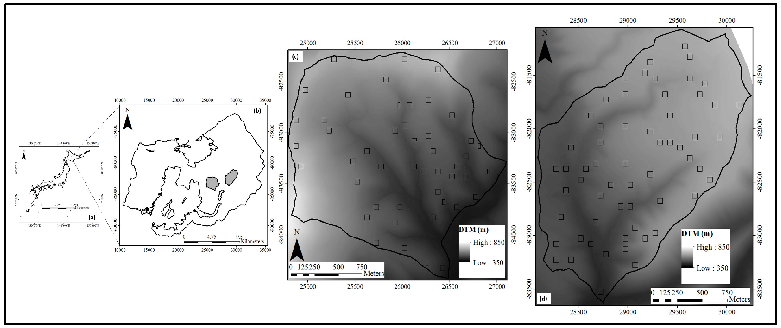
2.1. Study Site
2.2. Data Collection
2.2.1. Field Data
2.2.2. LiDAR Data
2.2.3. UAV Imagery
UAV Equipment and Payload
UAV Imagery Collection: Planning and Implementation
2.3. Data Analysis
2.3.1. Photogrammetric Processing
2.3.2. Generation and Comparison of LiDAR and UAV-SfM CHMs
Generation of LiDAR Canopy Height
Generation of UAV-SfM Canopy Height
Comparison of LiDARCHM and UAV-SfMCHM
2.3.3. Extraction and Comparison of Forest Structural Metrics
- Maximum height (MaxH)
- Mean height (MeanH)
- Standard deviation of heights, also known as the rugosity index [24] (SD of H)
- Coefficient of variation (CV of H)
- Skewness and Kurtosis
- Percentile heights of 10%, 25%, 50%, 75% and 95% (P10, P25, P50, P75 and P95)
- Canopy cover above 2 m height calculated as the proportion of points above 2 m height to the total number of points (d0)
- Density of points at 1st, 2nd, …, 9th height fractions (d1, d2, …, d9)
- Canopy cover above mean height calculated as the proportion of points above mean height to the total number of points (dmean)
- Surface area ratio that is the proportion of 3D canopy surface area to the ground surface area. Also known as “rumple index” [24].
2.3.4. Evaluation of the Utility of UAV-SfM-Derived Point Cloud Products and Plot-Level Validation of Canopy Height
2.3.5. Identification of Factors that Affect the Performance of UAV-SfMCHM
3. Results
3.1. Comparison of LiDAR and UAV-SfM Outputs
3.1.1. LiDAR and UAV-SfM Point Cloud Properties
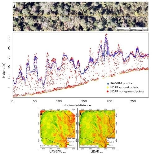
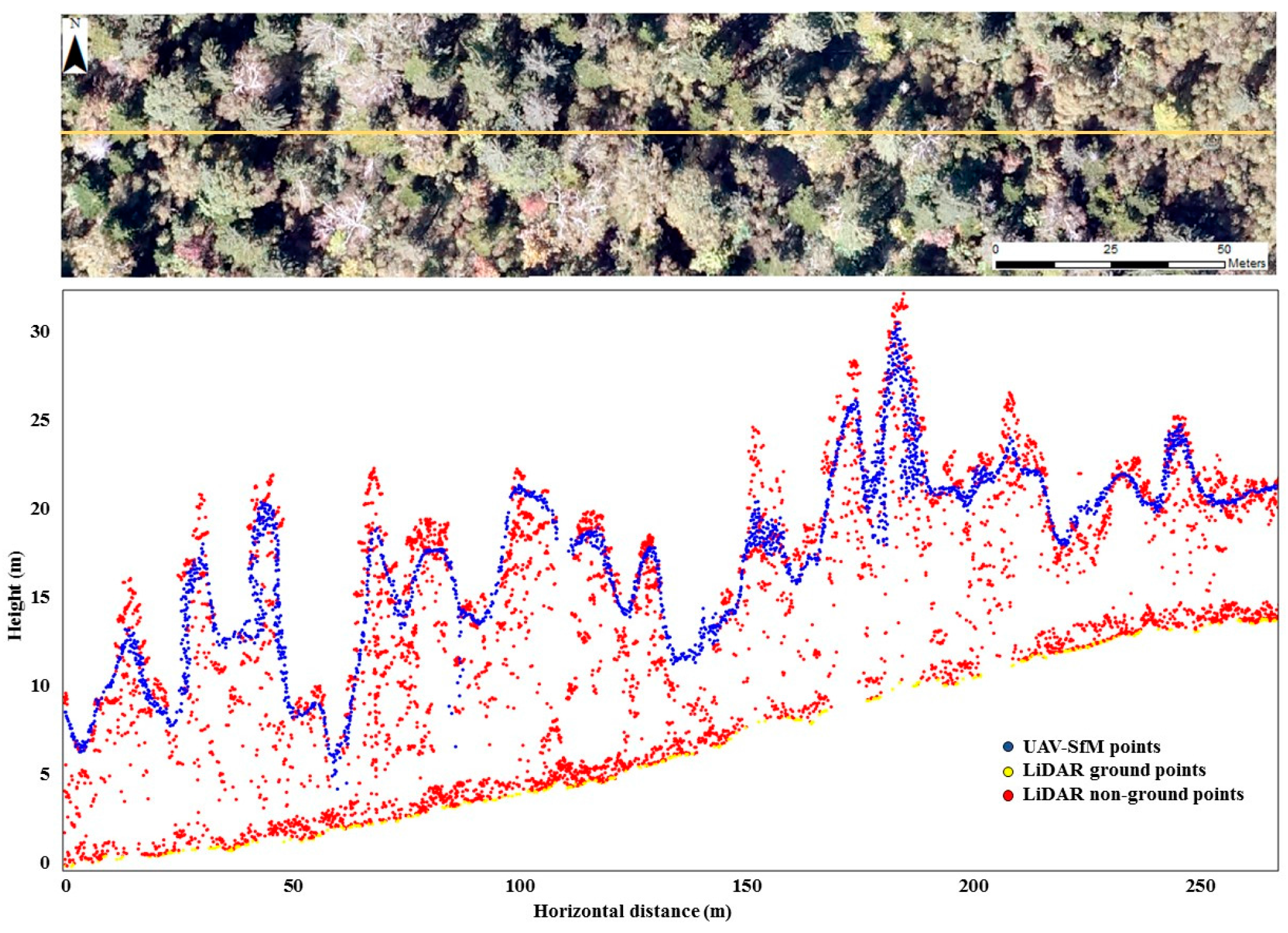
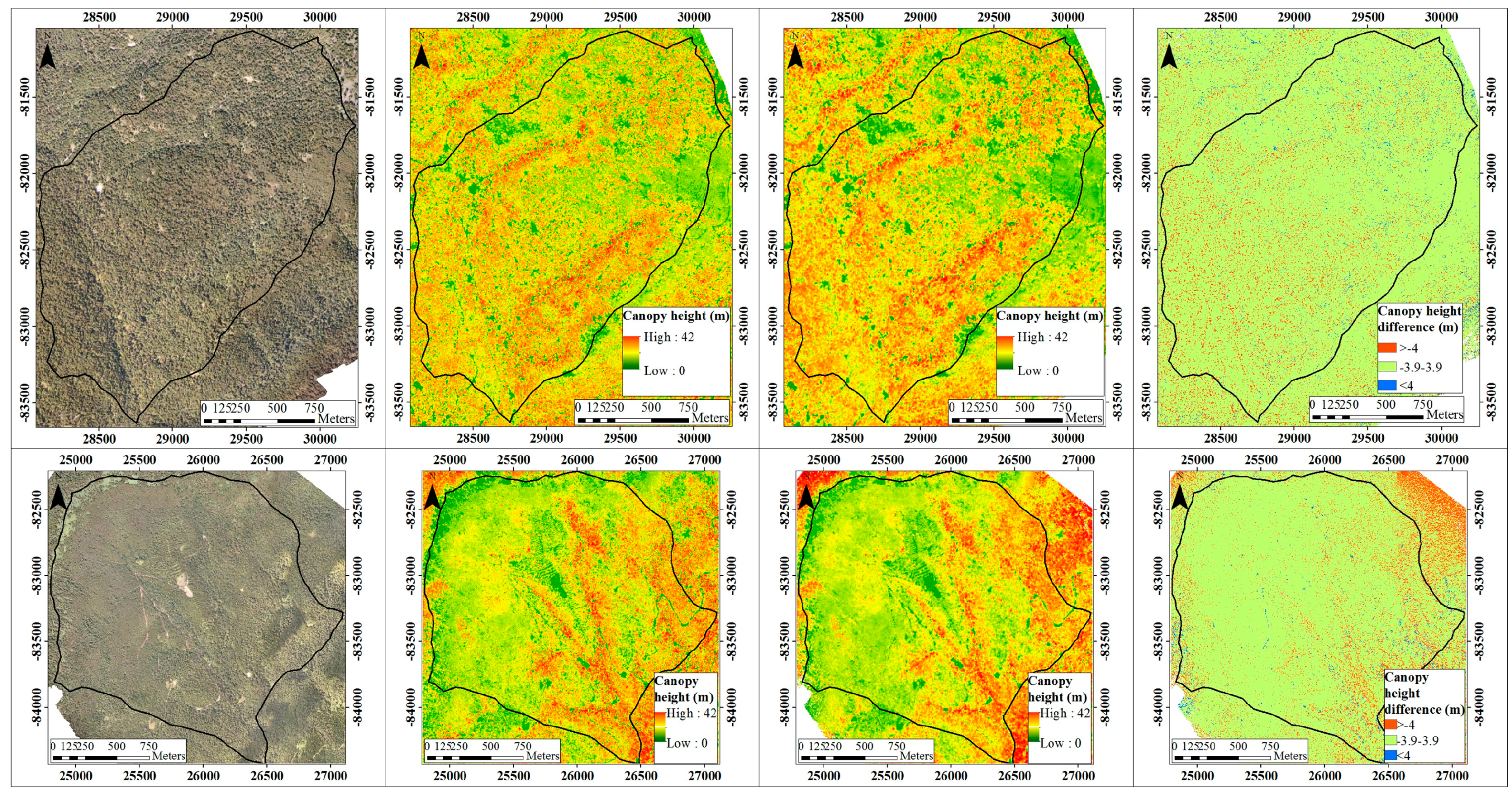
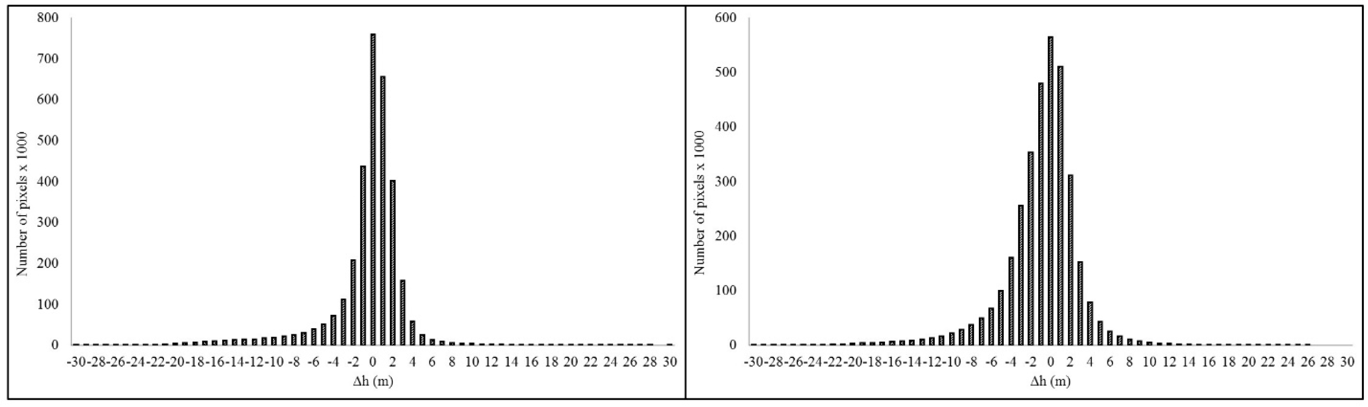
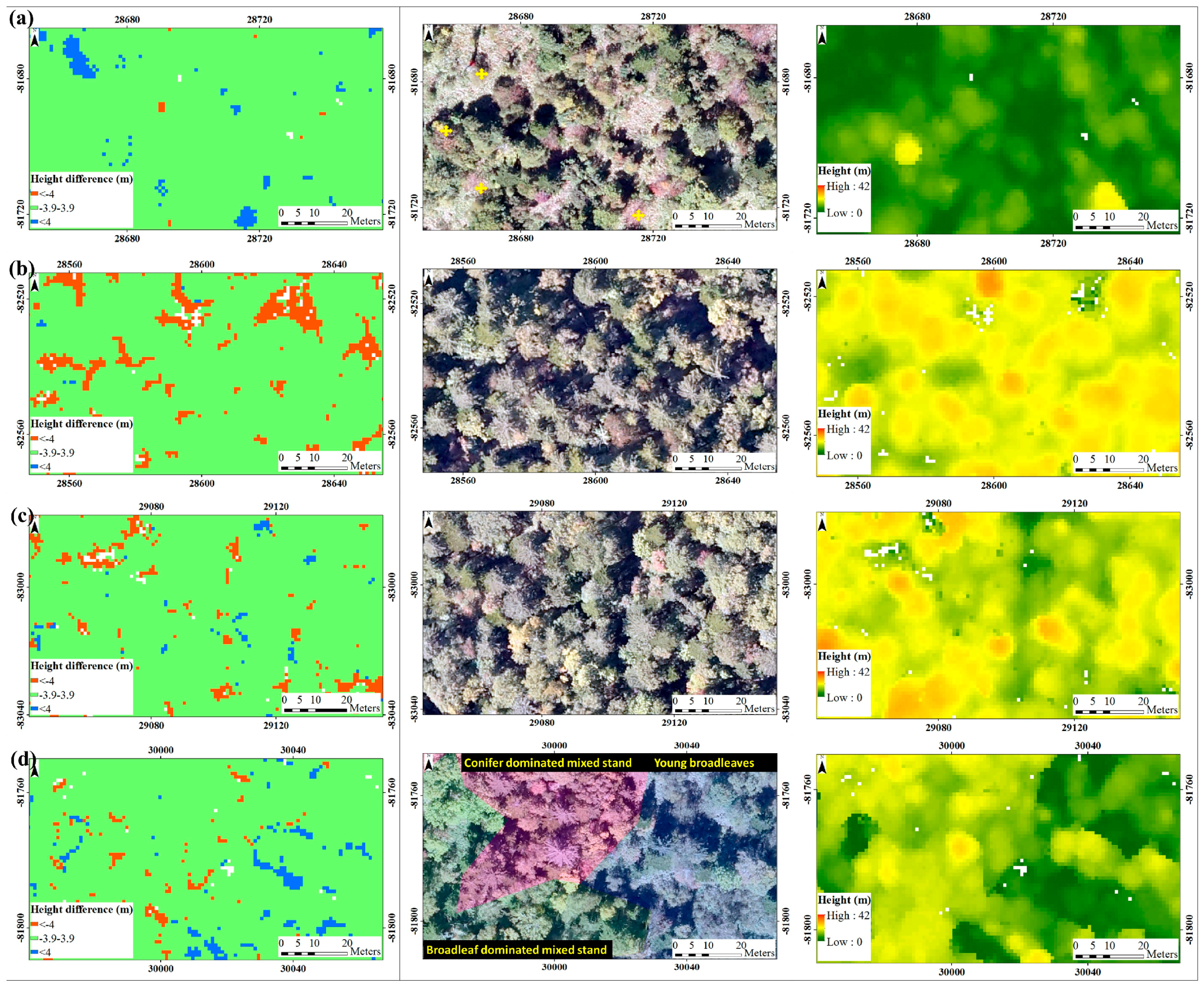
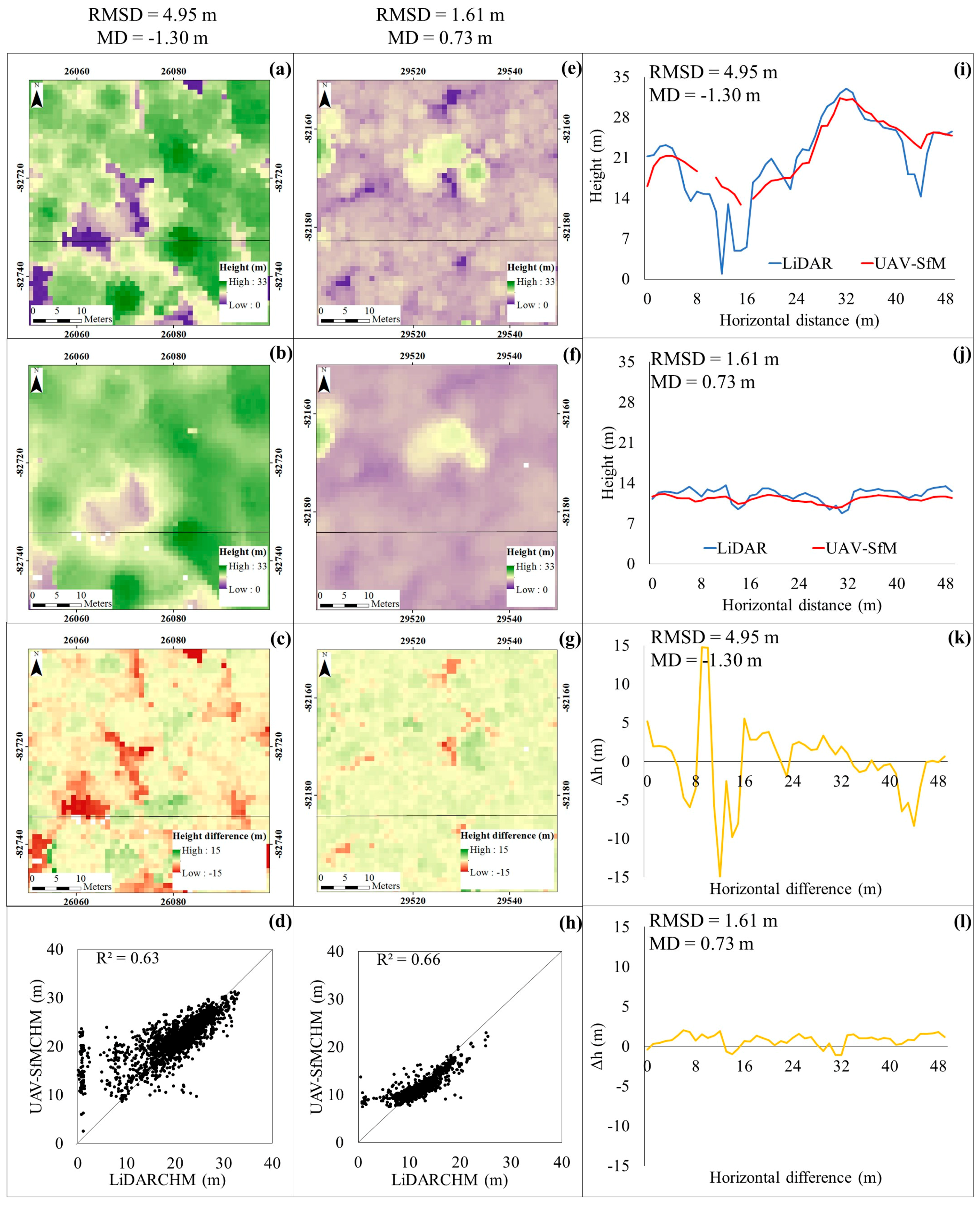
3.1.2. LiDAR and UAV-SfM CHMs
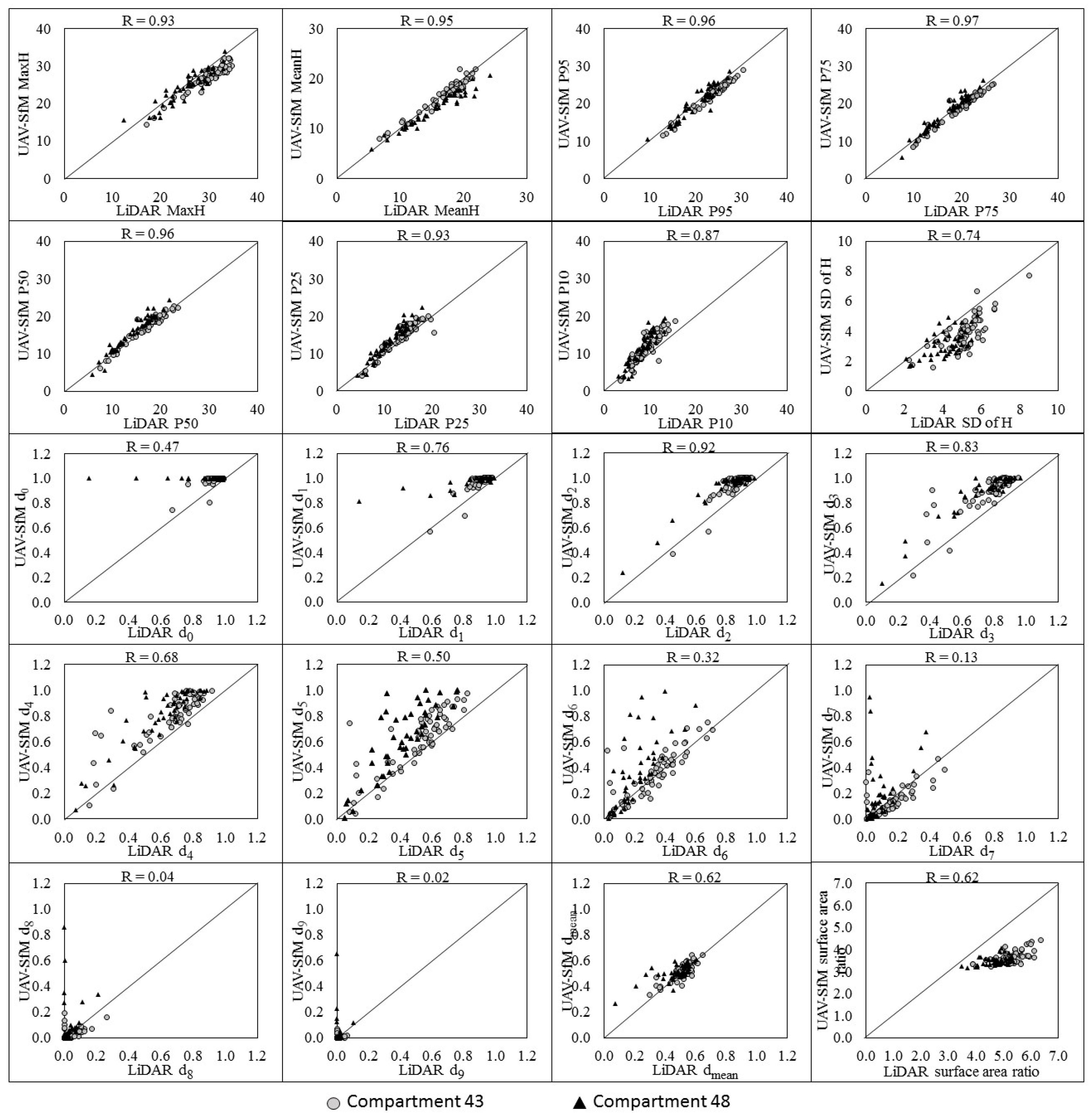
3.2. Comparison of Structural Metrics Derived from Photogrametric Products
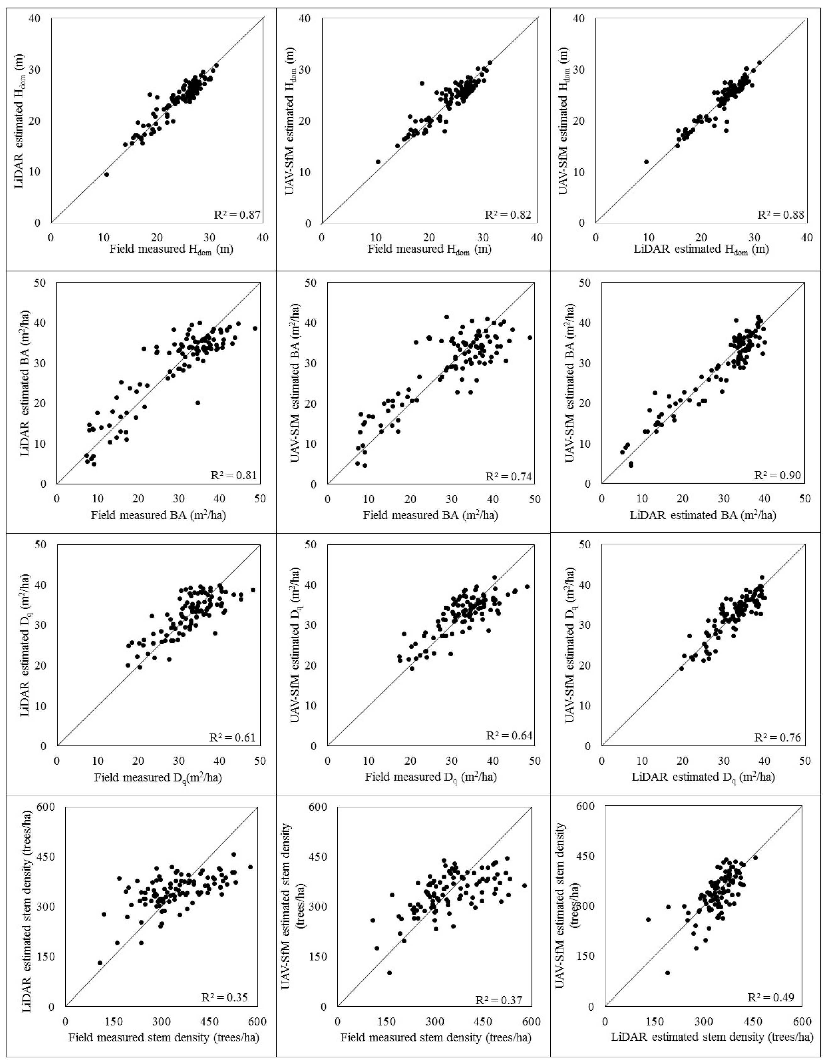
3.3. Regression Modelling and Plot-Level Validation of Forest Structural Attributes
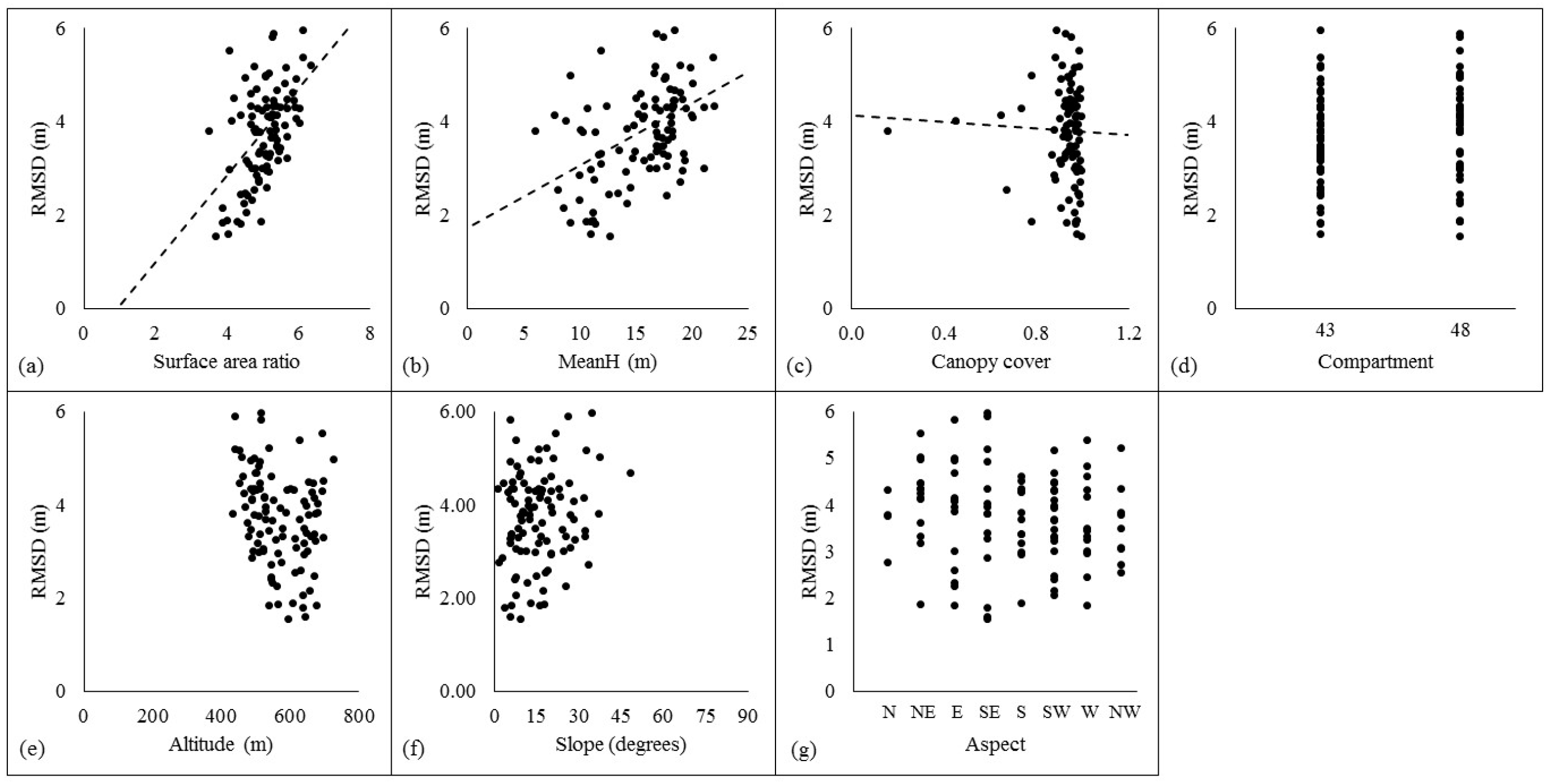
3.4. Factors that Affect the Performance of UAV-SfMCHM
4. Discussion
4.1. Characterisation of Forest Canopy Using the UAV-SfM Technique
4.2. Estimation and Plot-Level Validation of Forest Structural Attributes
4.3. Influence of Forest Structural Properties and Topographic Conditions on the Performance of Canopy Height Models
4.4. General Considerations for Forestry Applications
5. Conclusions
Acknowledgments
Author Contributions
Conflicts of Interest
References
- Spies, T. Forest Structure: A Key to the Ecosystem. Northwest Sci. 1998, 72, 34–39. [Google Scholar]
- McElhinny, C.; Gibbons, P.; Brack, C.; Bauhus, J. Forest and woodland stand structural complexity: Its definition and measurement. For. Ecol. Manag. 2005, 218, 1–24. [Google Scholar] [CrossRef]
- Nadkarni, N.M. Diversity of species and interactions in the upper tree canopy of forest ecosystems. Am. Zool. 1994, 78, 70–78. [Google Scholar] [CrossRef]
- Carswell, F.E.; Meir, P.; Wandelli, E.V.; Bonates, L.C.M.; Kruijt, B.; Barbosa, E.M.; Nobre, A.D.; Grace, J.; Jarvis, P.G. Photosynthetic capacity in a central Amazonian rain forest. Tree Physiol. 2000, 20, 179–186. [Google Scholar] [CrossRef] [PubMed]
- Lindenmayer, D.B.; Margules, C.R.; Botkin, D.B. Indicators of biodiversity for ecologically sustainable forest management. Conserv. Biol. 2001, 14, 941–950. [Google Scholar] [CrossRef]
- McElhinny, C.; Gibbons, P.; Brack, C. An objective and quantitative methodology for constructing an index of stand structural complexity. For. Ecol. Manag. 2006, 235, 54–71. [Google Scholar] [CrossRef]
- Levesque, J.; King, D.J. Spatial analysis of radiometeric fractions from high resolution multispectral imagery for modellling individual tree crown and forest canopy structure and health. Remote Sens. Environ. 2003, 84, 589–602. [Google Scholar] [CrossRef]
- Franklin, J.F.; Van Pelt, R. Spatial aspects of structural complexity in old-growth forests. J. For. 2004, 102, 22–28. [Google Scholar]
- Kane, V.R.; McGaughey, R.J.; Bakker, J.D.; Gersonde, R.F.; Lutz, J.A.; Franklin, J.F. Comparisons between field- and LiDAR-based measures of stand structural complexity. Can. J. For. Res. 2010, 40, 761–773. [Google Scholar] [CrossRef]
- Lowman, M.D.; Wittman, P.K. Forest canopies: Methods, hypotheses, and future directions, a brief history of methods of access. Annu. Rev. Ecol. 1996, 27, 55–81. [Google Scholar] [CrossRef]
- Barker, M.G.; Pinard, M.A. Forest canopy research: Sampling problems, and some solutions. Plant Ecol. 2001, 153, 23–38. [Google Scholar] [CrossRef]
- Ma, Z.; Hart, M.M.; Redmond, R.L. Mapping vegetation across large geographic areas: Integration of remote sensing and GIS to classify multisource data. Eng. Remote Sens. 2001, 67, 295–307. [Google Scholar]
- Xie, Y.; Sha, Z.; Yu, M. Remote sensing imagery in vegetation mapping: A review. J. Plant Ecol. 2008, 1, 9–23. [Google Scholar] [CrossRef]
- Kane, V.R.; Bakker, J.D.; McGaughey, R.J.; Lutz, J.A.; Gersonde, R.F.; Franklin, J.F. Examining conifer canopy structural complexity across forest ages and elevations with LiDAR data. Can. J. For. Res. 2010, 40, 774–787. [Google Scholar] [CrossRef]
- Leberl, F.; Irschara, A.; Pock, T.; Meixner, P.; Gruber, M.; Scholz, S.; Wiechert, A. Point clouds: LiDAR versus 3D vision. Photogramm. Eng. Remote Sens. 2010, 76, 1123–1134. [Google Scholar] [CrossRef]
- Hyyppä, J.; Yu, X.; Hyyppä, H.; Vastaranta, M.; Holopainen, M.; Kukko, A.; Kaartinen, H.; Jaakkola, A.; Vaaja, M.; Koskinen, J.; et al. Advances in forest inventory using airborne laser scanning. Remote Sens. 2012, 4, 1190–1207. [Google Scholar] [CrossRef]
- Wulder, M.A.; Coops, N.C.; Hudak, A.T.; Morsdorf, F.; Nelson, R.F.; Newnham, G.J.; Vastaranta, M. Status and prospects for LiDAR remote sensing of forested ecosystems.pdf. Can. J. Remote Sens. 2013, 39, S1–S5. [Google Scholar] [CrossRef]
- Anderson, K.; Gaston, K.J. Lightweight unmanned aerial vehicles will revolutionize spatial ecology. Front. Ecol. Environ. 2013, 11, 138–146. [Google Scholar] [CrossRef]
- Lisein, J.; Pierrot-Deseilligny, M.; Bonnet, S.; Lejeune, P. A photogrammetric workflow for the creation of a forest canopy height model from small unmanned aerial system imagery. Forests 2013, 4, 922–944. [Google Scholar] [CrossRef]
- Zellweger, F.; Braunisch, V.; Baltensweiler, A.; Bollmann, K. Remotely sensed forest structural complexity predicts multi species occurrence at the landscape scale. For. Ecol. Manag. 2013, 307, 303–312. [Google Scholar] [CrossRef]
- Salamí, E.; Barrado, C.; Pastor, E. UAV flight experiments applied to the remote sensing of vegetated areas. Remote Sens. 2014, 6, 11051–11081. [Google Scholar] [CrossRef]
- Torresan, C.; Berton, A.; Carotenuto, F.; Genaro, S.F.D.; Gioli, B.; Matese, A.; Miglietta, F.; Vagnoli, C.; Zaldei, A.; Wallace, L. Forestry applications of UAVs in Europe: A review Forestry applications of UAVs in Europe: A review. Int. J. Remote Sens. 2017, 38, 2427–2447. [Google Scholar] [CrossRef]
- Lefsky, M.A.; Cohen, W.B.; Parker, G.G.; Harding, D.J. LiDAR Remote Sensing for Ecosystem Studies. Bioscience 2002, 52, 19–30. [Google Scholar] [CrossRef]
- Parker, G.G.; Harmon, M.E.; Lefsky, M.A.; Chen, J.; Van Pelt, R.; Weis, S.B.; Thomas, S.C.; Winner, W.E.; Shaw, D.C.; Frankling, J.F. Three-dimensional Structure of an Old-growth Pseudotsuga-Tsuga Canopy and Its Implications for Radiation Balance, Microclimate, and Gas Exchange. Ecosystems 2004, 7, 440–453. [Google Scholar] [CrossRef]
- Næsset, E. Predicting forest stand characteristics with airborne scanning laser using a practical two-stage procedure and field data. Remote Sens. Environ. 2002, 80, 88–99. [Google Scholar] [CrossRef]
- Næsset, E.; Gobakken, T.; Holmgren, J.; Hyyppä, H.; Hyyppä, J.; Maltamo, M.; Nilsson, M.; Olsson, H.; Persson, Å.; Söderman, U. Laser scanning of forest resources: The nordic experience. Scand. J. For. Res. 2004, 19, 482–499. [Google Scholar] [CrossRef]
- Maltamo, M.; Packalén, P.; Yu, X.; Eerikäinen, K.; Hyyppä, J.; Pitkänen, J. Identifying and quantifying structural characteristics of heterogeneous boreal forests using laser scanner data. For. Ecol. Manag. 2005, 216, 41–50. [Google Scholar] [CrossRef]
- Reitberger, J.; Krzystek, P.; Stilla, U. Analysis of full waveform LiDAR data for the classification of deciduous and coniferous trees. Int. J. Remote Sens. 2008, 29, 1407–1431. [Google Scholar] [CrossRef]
- Wolf, P.; Dewitt, B. Elements of Photogrammetry with Applications in GIS, 3rd ed.; McGraw-Hill: New York, NY, USA, 2000. [Google Scholar]
- Grenzdörffer, G.J.; Engel, A.; Teichert, B. The Photogrammetric potential of low-cost UAVs in forestry and agriculture. Int. Arch. Photogramm. Remote Sens. Spat. Inf. Sci. 2008, 31, 1207–2014. [Google Scholar] [CrossRef]
- Jaakkola, A.; Hyyppä, J.; Yu, X.; Kukko, A.; Kaartinen, H.; Liang, X.; Hyyppä, H.; Wang, Y. Autonomous collection of forest field reference—The outlook and a first step with UAV laser scanning. Remote Sens. 2017, 9, 785. [Google Scholar] [CrossRef]
- Fryskowska, A.; Kedzierski, M.; Walczykowski, P.; Wierzbicki, D.; Delis, P.; Lada, A. Effective detection of sub-surface archeological features from laser scanning point clouds and imagery data. Int. Arch. Photogramm. Remote Sens. Spat. Inf. Sci. 2017, XLII-2/W5, 245–251. [Google Scholar] [CrossRef]
- Honkavaara, E.; Saari, H.; Kaivosoja, J.; Pölönen, I.; Hakala, T.; Litkey, P.; Mäkynen, J.; Pesonen, L. Processing and assessment of spectrometric, stereoscopic imagery collected using a lightweight UAV spectral camera for precision agriculture. Remote Sens. 2013, 5, 5006–5039. [Google Scholar] [CrossRef]
- Näsi, R.; Honkavaara, E.; Lyytikäinen-Saarenmaa, P.; Blomqvist, M.; Litkey, P.; Hakala, T.; Viljanen, N.; Kantola, T.; Tanhuanpää, T.; Holopainen, M. Using UAV-based photogrammetry and hyperspectral imaging for mapping bark beetle damage at tree-level. Remote Sens. 2015, 7, 15467–15493. [Google Scholar] [CrossRef]
- Järnstedt, J.; Pekkarinen, A.; Tuominen, S.; Ginzler, C.; Holopainen, M.; Viitala, R. Forest variable estimation using a high-resolution digital surface model. ISPRS J. Photogramm. Remote Sens. 2012, 74, 78–84. [Google Scholar] [CrossRef]
- Bohlin, J.; Wallerman, J.; Fransson, J.E.S. Forest variable estimation using photogrammetric matching of digital aerial images in combination with a high-resolution DEM. Scand. J. For. Res. 2012, 27, 692–699. [Google Scholar] [CrossRef]
- Nurminen, K.; Karjalainen, M.; Yu, X.; Hyyppä, J.; Honkavaara, E. Performance of dense digital surface models based on image matching in the estimation of plot-level forest variables. ISPRS J. Photogramm. Remote Sens. 2013, 83, 104–115. [Google Scholar] [CrossRef]
- Puliti, S.; Olerka, H.; Gobakken, T.; Næsset, E. Inventory of small forest areas using an unmanned aerial system. Remote Sens. 2015, 7, 9632–9654. [Google Scholar] [CrossRef]
- Wallace, L.; Lucieer, A.; Malenovský, Z.; Turner, D.; Petr, V. Assessment of forest structure using two UAV techniques: A comparison of airborne laser scanning and structure from motion (SfM) point clouds. Forests 2016, 7, 62. [Google Scholar] [CrossRef]
- Gobakken, T.; Bollandsås, O.M.; Næsset, E. Comparing biophysical forest characteristics estimated from photogrammetric matching of aerial images and airborne laser scanning data. Scand. J. For. Res. 2015, 30, 73–86. [Google Scholar] [CrossRef]
- Mlambo, R.; Woodhouse, I.H.; Gerard, F.; Anderson, K. Structure from motion (SfM) photogrammetry with drone data: A low cost method for monitoring greenhouse gas emissions from forests in developing countries. Forests 2017, 8, 68. [Google Scholar] [CrossRef]
- Yu, X.; Hyyppä, J.; Karjalainen, M.; Nurminen, K.; Karila, K.; Vastaranta, M.; Kankare, V.; Kaartinen, H.; Holopainen, M.; Honkavaara, E.; et al. Comparison of laser and stereo optical, SAR and InSAR point clouds from air- and space-borne sources in the retrieval of forest inventory attributes. Remote Sens. 2015, 7, 15933–15954. [Google Scholar] [CrossRef]
- White, J.; Stepper, C.; Tompalski, P.; Coops, N.; Wulder, M.A. Comparing ALS and image-based point cloud metrics and modelled forest inventory attributes in a complex coastal forest environment. Forests 2015, 6, 3704–3732. [Google Scholar] [CrossRef]
- Thiel, C.; Schmullius, C. Comparison of UAV photograph-based and airborne LiDAR-based point clouds over forest from a forestry application perspective. Int. J. Remote Sens. 2017, 38, 2411–2426. [Google Scholar] [CrossRef]
- Puliti, S.; Ene, L.T.; Gobakken, T.; Næsset, E. Use of partial-coverage UAV data in sampling for large scale forest inventories. Remote Sens. Environ. 2017, 194, 115–126. [Google Scholar] [CrossRef]
- Jensen, J.; Mathews, A. Assessment of image-based point cloud products to generate a bare earth surface and estimate canopy heights in a woodland ecosystem. Remote Sens. 2016, 8, 50. [Google Scholar] [CrossRef]
- Hernández-Clemente, R.; Navarro-Cerrillo, R.M.; Romero Ramírez, F.J.; Hornero, A.; Zarco-Tejada, P.J. A novel methodology to estimate single-tree biophysical parameters from 3D digital imagery compared to aerial laser scanner data. Remote Sens. 2014, 6, 11627–11648. [Google Scholar] [CrossRef]
- Wong, W.V.C.; Tsuyuki, S.; Phua, M.; Ioki, K.; Takao, G. Performance of a photogrammetric digital elevation model in a tropical montane forest environment. J. For. Plan. 2016, 21, 39–52. [Google Scholar]
- Widyaningrum, E.; Gorte, B.G.H. Comprehensive comparison of two image-based point clouds from aerial photos with airborne LiDAR for large-scale mapping. Int. Arch. Photogramm. Remote Sens. Spat. Inf. Sci. 2017, 42, 557–565. [Google Scholar] [CrossRef]
- Baltsavias, E.; Gruen, A.; Eisenbeiss, H.; Zhang, L.; Waser, L.T. High-quality image matching and automated generation of 3D tree models. Int. J. Remote Sens. 2008, 29, 1243–1259. [Google Scholar] [CrossRef]
- Dandois, J.P.; Ellis, E.C. Remote sensing of vegetation structure using computer vision. Remote Sens. 2010, 2, 1157–1176. [Google Scholar] [CrossRef]
- Zarco-Tejada, P.J.; Diaz-Varela, R.; Angileri, V.; Loudjani, P. Tree height quantification using very high resolution imagery acquired from an unmanned aerial vehicle (UAV) and automatic 3D photo-reconstruction methods. Eur. J. Agron. 2014, 55, 89–99. [Google Scholar] [CrossRef]
- Matese, A.; Toscano, P.; Di Gennaro, S.F.; Genesio, L.; Vaccari, F.P.; Primicerio, J.; Belli, C.; Zaldei, A.; Bianconi, R.; Gioli, B. Intercomparison of UAV, aircraft and satellite remote sensing platforms for precision viticulture. Remote Sens. 2015, 7, 2971–2990. [Google Scholar] [CrossRef]
- Nex, F.; Remondino, F. UAV for 3D mapping applications: A review. Appl. Geomat. 2014, 6, 1–15. [Google Scholar] [CrossRef]
- Tuominen, S.; Balazs, A.; Saari, H.; Pölönen, I.; Sarkeala, J.; Viitala, R. Unmanned aerial system imagery and photogrammetric canopy height data in area-based estimation of forest variables. Silva Fenn. 2015, 49, 1348. [Google Scholar] [CrossRef]
- Müller, J.; Gärtner-Roer, I.; Thee, P.; Ginzler, C. Accuracy assessment of airborne photogrammetrically derived high-resolution digital elevation models in a high mountain environment. ISPRS J. Photogramm. Remote Sens. 2014, 98, 58–69. [Google Scholar] [CrossRef]
- Owari, T.; Kamata, N.; Tange, T.; Kaji, M.; Shimomura, A. Effects of silviculture treatments in a hurricane-damaged forest on carbon storage and emissions in central Hokkaido, Japan. J. For. Res. 2011, 22, 13–20. [Google Scholar] [CrossRef]
- Tatewaki, M. Forest Ecology of the Islands of the North Pacific Ocean. J. Fac. Agric. Hokkaido Univ. 1958, 50, 371–486. [Google Scholar]
- The University of Tokyo Hokkaido Forest. 2017. Available online: http://www.uf.a.u-tokyo.ac.jp/files/gaiyo_hokkaido.pdf. (accessed on 24 October 2017).
- Horie, K.; Miyamoto, Y.; Limura, N.; Oikawa, N. List of Vascular Plant of the University of Tokyo Hokkaido Forest. 2013, Volume 54. Available online: https://repository.dl.itc.u-tokyo.ac.jp/?action=pages_view_main&active_action=repository_view_main_item_detail&item_id=26164&item_no=1&page_id=28&block_id=31 (accessed on 24 October 2017).
- Verhoeven, G.; Doneus, M.; Briese, C.; Vermeulen, F. Mapping by matching: A computer vision-based approach to fast and accurate georeferencing of archaeological aerial photographs. J. Archaeol. Sci. 2012, 39, 2060–2070. [Google Scholar] [CrossRef]
- Remondino, F.; Spera, M.G.; Nocerino, E.; Menna, F.; Nex, F. State of the art in high density image matching. Photogramm. Rec. 2014, 29, 144–166. [Google Scholar] [CrossRef]
- Ota, T.; Ogawa, M.; Shimizu, K.; Kajisa, T.; Mizoue, N.; Yoshida, S.; Takao, G.; Hirata, Y.; Furuya, N.; Sano, T.; et al. Aboveground biomass estimation using structure from motion approach with aerial photographs in a seasonal tropical forest. Forests 2015, 6, 3882–3898. [Google Scholar] [CrossRef]
- McGaughey, R. FUSION/LDV: Software for LiDAR Data Analysis and Visualization; USDA Forest Service Pacific Northwest Research Station: Seattle, WA, USA, 2016; p. 211.
- Jayathunga, S.; Owari, T.; Tsuyuki, S. Analysis of forest structural complexity using airborne LiDAR data and aerial photography in a mixed conifer–broadleaf forest in northern Japan. J. For. Res. 2017. [Google Scholar] [CrossRef]
- Sona, G.; Pinto, L.; Pagliari, D.; Passoni, D.; Gini, R. Experimental analysis of different software packages for orientation and digital surface modelling from UAV images. Earth Sci. Inform. 2014, 7, 97–107. [Google Scholar] [CrossRef]
- Meißner, H.; Cramer, M.; Piltz, B. Benchmarking the optical resolving power of uav based camera. Int. Arch. Photogramm. Remote Sens. Spat. Inf. Sci. 2017, XLII, 4–7. [Google Scholar] [CrossRef]
- Kedzierski, M.; Wierzbicki, D. Radiometric quality assessment of images acquired by UAV’s in various lighting and weather conditions. Meas. J. Int. Meas. Confed. 2015, 76, 156–169. [Google Scholar] [CrossRef]
- Khosravipour, A.; Skidmore, A.K.; Wang, T.; Isenburg, M.; Khoshelham, K. Effect of slope on treetop detection using a LiDAR canopy height model. ISPRS J. Photogramm. Remote Sens. 2015, 104, 44–52. [Google Scholar] [CrossRef]


| Compartment | 43 | 48 |
|---|---|---|
| Total area (ha) | 335 | 340 |
| Altitude range (m a.s.l.) | 425 to 810 | 397 to 833 |
| Date of ground survey | March, 2016 | March, 2017 |
| Total number of sample plots (plot size) | 59 (0.25 ha) | 46 (40 of 0.25 ha and 6 of 0.125 ha) |
| Compartment 43 | Compartment 48 | ||
|---|---|---|---|
| Average (SD) Values | Average (SD) Values | ||
| Dominant Height (m) | 25.5 (3.5) | 22.0 (4.3) | |
| For trees with DBH ≥ 14 cm | Mean DBH (cm) | 32.3 (4.6) | 14.9 (4.1) |
| Gross volume (m3/ha) | 286.5 (91.6) | 207.5 (105.0) | |
| BA (m2/ha) | 32.2 (9.6) | 24.4 (110.0) | |
| Stem density (trees/ha) | 324 (93) | 366 (102) | |
| Proportion of conifer stems | 0.46 (0.16) | 0.26 (0.20) | |
| Only for canopy trees | Mean DBH (cm) | 36.5 (14.9) | 34.3 (11.0) |
| Gross volume (m3/ha) | 211.2 (61.7) | 177.0 (82.9) | |
| BA (m2/ha) | 21.6 (5.7) | 19.8 (7.9) | |
| Stem density (trees/ha) | 124 (57) | 218 (105) | |
| Proportion of conifer stems | 0.55 (0.20) | 0.30 (0.23) | |
| Parameter | Description |
|---|---|
| Nominal flying height | 600 m |
| Flying speed | 140 km/h |
| Course overlap | 50% |
| Pulse rate | 100 kHz |
| Scan angle | ±20° |
| Beam divergence | 0.16 mrad |
| Point density | 8.4 pts./m2 |
| Structural Metrics | Compartment 43 | Compartment 48 | ||||||
|---|---|---|---|---|---|---|---|---|
| LiDAR Mean (SD) | UAV-SfM Mean (SD) | MD (SD of Difference) | RMSD | LiDAR Mean (SD) | UAV-SfM Mean (SD) | MD (SD of Difference) | RMSD | |
| MaxH (m) | 30.00 (3.72) | 27.05 (3.49) | 2.96 (1.14) | 2.69 | 25.41 (4.54) | 24.37 (4.36) | 1.05 (1.84) | 2.24 |
| MeanH (m) | 16.78 (3.21) | 17.07 (3.53) | −0.29 (0.93) | 1.12 | 13.90 (3.43) | 15.42 (4.31) | −1.52 (1.25) | 2.34 |
| SD of H (m) | 5.19 (0.99) | 3.86 (1.15) | 1.34 (0.78) | 1.47 | 4.18 (0.92) | 3.16 (0.87) | 1.02 (0.77) | 1.24 |
| CV of H (m) | 0.32 (0.06) | 0.24 (0.09) | 0.08 (0.10) | 0.13 | 0.31 (0.06) | 0.22 (0.10) | 0.09 (0.06) | 0.08 |
| Skewness | −0.46 (0.56) | −0.35 (0.68) | −0.12 (0.42) | 0.69 | −0.22 (0.53) | −0.15 (0.73) | −0.07 (0.52) | 0.70 |
| Kurtosis | 3.26 (0.88) | 3.64 (1.27) | −0.38 (0.98) | 1.49 | 3.23 (0.73) | 3.65 (1.55) | −0.42 (1.36) | 2.41 |
| P10 (m) | 9.46 (2.53) | 11.97 (3.83) | −2.51 (2.11) | 3.39 | 8.30 (2.53) | 11.33 (4.22) | −3.03 (2.12) | 3.82 |
| P25 (m) | 13.68 (3.28) | 14.71 (3.68) | −1.03 (1.40) | 2.07 | 11.30 (3.30) | 13.41 (4.45) | −2.11 (1.56) | 2.79 |
| P50 (m) | 17.44 (3.73) | 17.41 (3.83) | 0.03 (0.74) | 0.80 | 14.18 (3.80) | 15.48 (4.55) | −1.30 (1.24) | 2.13 |
| P75 (m) | 20.39 (3.91) | 19.69 (3.84) | 0.70 (0.62) | 0.91 | 16.74 (4.07) | 17.52 (4.52) | 1.07 (0.07) | 1.74 |
| P95 (m) | 24.25 (3.53) | 22.87 (3.50) | 1.38 (0.57) | 1.21 | 20.41 (4.05) | 20.46 (4.44) | 1.40 (0.40) | 1.95 |
| d0 | 0.94 (0.05) | 0.99 (0.04) | −0.05 (0.03) | 0.05 | 0.91 (0.15) | 1.00 (0.00) | −0.09 (0.15) | 0.34 |
| d1 | 0.92 (0.06) | 0.97 (0.07) | −0.05 (0.04) | 0.06 | 0.89 (0.16) | 0.98 (0.04) | −0.10 (0.12) | 0.28 |
| d2 | 0.89 (0.08) | 0.95 (0.10) | −0.06 (0.04) | 0.07 | 0.85 (0.18) | 0.94 (0.14) | −0.10 (0.06) | 0.12 |
| d3 | 0.85 (0.11) | 0.93 (0.14) | −0.07 (0.06) | 0.09 | 0.79 (0.21) | 0.91 (0.18) | −0.12 (0.06) | 0.14 |
| d4 | 0.78 (0.16) | 0.87 (0.21) | −0.09 (0.07) | 0.10 | 0.70 (0.24) | 0.84 (0.23) | −0.15 (0.06) | 0.15 |
| d5 | 0.71 (0.21) | 0.80 (0.27) | −0.09 (0.07) | 0.11 | 0.58 (0.27) | 0.73 (0.30) | −0.15 (0.08) | 0.16 |
| d6 | 0.63 (0.23) | 0.73 (0.29) | −0.10 (0.08) | 0.14 | 0.46 (0.29) | 0.59 (0.36) | −0.13 (0.10) | 0.16 |
| d7 | 0.55 (0.23) | 0.64 (0.29) | −0.08 (0.09) | 0.14 | 0.34 (0.26) | 0.47 (0.37) | −0.12 (0.13) | 0.22 |
| d8 | 0.45 (0.21) | 0.50 (0.26) | −0.05 (0.09) | 0.12 | 0.24 (0.22) | 0.35 (0.32) | −0.11 (0.14) | 0.25 |
| d9 | 0.33 (0.18) | 0.33 (0.21) | 0.00 (0.06) | 0.07 | 0.14 (0.15) | 0.22 (0.25) | −0.08 (0.14) | 0.24 |
| dmean | 0.51 (0.06) | 0.52 (0.06) | −0.01 (0.04) | 0.05 | 0.48 (0.10) | 0.51 (0.06) | −0.03 (0.07) | 0.11 |
| Surface area ratio | 5.27 (0.54) | 3.67 (0.28) | 1.60 (0.43) | 1.15 | 4.74 (0.44) | 3.48 (0.19) | 1.26 (0.40) | 0.97 |
| Explanatory Variable a | RMSE b | RMSE% c | |
|---|---|---|---|
| Dominant height (hdom) | |||
| LiDAR model | P95, d2 | 1.50 m | 6.26 |
| UAV-SfM model | P75, SD of H, d1 | 1.78 m | 7.43 |
| Basal area (BA) | |||
| LiDAR model | MaxH, d6 | 4.58 m2/ha | 15.82 |
| UAV-SfM model | SD of H, P95, dmean | 5.42 m2/ha | 18.74 |
| Quadratic mean DBH (Dq) | |||
| LiDAR model | MaxH, P10, d1 | 3.75 cm | 11.54 |
| UAV-SfM model | P95, d1 | 3.92 cm | 12.07 |
| Stem density (N) | |||
| LiDAR model | P10, d1, d8 | 76 trees/ha | 22.26 |
| UAV-SfM model | SD of H, d1, d8, dmean | 78 trees/ha | 22.67 |
| Variable | Coefficient | Standard Error | t Value | p Value |
|---|---|---|---|---|
| (Intercept) | −0.48 | 1.68 | −0.28 | 0.778 |
| Altitude | 0.00 | 0.00 | −0.52 | 0.605 |
| Aspect (North) | 0.26 | 0.44 | 0.58 | 0.565 |
| Aspect Northeast) | 0.04 | 0.29 | 0.15 | 0.881 |
| Aspect (Northwest) | −0.42 | 0.34 | −1.26 | 0.210 |
| Aspect (South) | −0.16 | 0.30 | −0.54 | 0.588 |
| Aspect Southeast) | 0.14 | 0.29 | 0.49 | 0.625 |
| Aspect (Southwest) | −0.18 | 0.28 | −0.65 | 0.515 |
| Aspect (West) | −0.14 | 0.31 | −0.47 | 0.643 |
| Slope | 0.01 | 0.01 | 1.10 | 0.273 |
| MeanH | 0.14 | 0.04 | 3.99 | 0.000 *** |
| Canopy cover | −2.85 | 0.90 | −3.17 | 0.002 ** |
| Surface area ratio | 0.91 | 0.20 | 4.57 | 0.000 *** |
| Compartment 48 | 0.99 | 0.21 | 4.82 | 0.000 *** |
© 2018 by the authors. Licensee MDPI, Basel, Switzerland. This article is an open access article distributed under the terms and conditions of the Creative Commons Attribution (CC BY) license (http://creativecommons.org/licenses/by/4.0/).
Share and Cite
Jayathunga, S.; Owari, T.; Tsuyuki, S. Evaluating the Performance of Photogrammetric Products Using Fixed-Wing UAV Imagery over a Mixed Conifer–Broadleaf Forest: Comparison with Airborne Laser Scanning. Remote Sens. 2018, 10, 187. https://doi.org/10.3390/rs10020187
Jayathunga S, Owari T, Tsuyuki S. Evaluating the Performance of Photogrammetric Products Using Fixed-Wing UAV Imagery over a Mixed Conifer–Broadleaf Forest: Comparison with Airborne Laser Scanning. Remote Sensing. 2018; 10(2):187. https://doi.org/10.3390/rs10020187
Chicago/Turabian StyleJayathunga, Sadeepa, Toshiaki Owari, and Satoshi Tsuyuki. 2018. "Evaluating the Performance of Photogrammetric Products Using Fixed-Wing UAV Imagery over a Mixed Conifer–Broadleaf Forest: Comparison with Airborne Laser Scanning" Remote Sensing 10, no. 2: 187. https://doi.org/10.3390/rs10020187
APA StyleJayathunga, S., Owari, T., & Tsuyuki, S. (2018). Evaluating the Performance of Photogrammetric Products Using Fixed-Wing UAV Imagery over a Mixed Conifer–Broadleaf Forest: Comparison with Airborne Laser Scanning. Remote Sensing, 10(2), 187. https://doi.org/10.3390/rs10020187