Article

The Use of Photogrammetry to Construct Time Series of Vegetation Permeability to Water and Seed Transport in Agricultural Waterways

1
LISAH, Univ Montpellier, INRA, IRD, Montpellier SupAgro, 34060 Montpellier, France
2
Ecosys, INRA - AgroParisTech, 78850 Thiverval-Grignon, France
3
G-Eau, Univ Montpellier, AgroParisTech, CIRAD, IRD, IRSTEA, Montpellier SupAgro, 34060 Montpellier, France
4
AgroParisTech, 75005 Paris, France
*
Author to whom correspondence should be addressed.
Remote Sens. 2018, 10(12), 2050; https://doi.org/10.3390/rs10122050
Submission received: 19 October 2018 / Revised: 30 November 2018 / Accepted: 12 December 2018 / Published: 17 December 2018
(This article belongs to the Special Issue High Resolution Image Time Series for Novel Agricultural Applications)

Abstract

:
Terrestrial vegetation has numerous positive effects on the main regulating services of agricultural channels, such as seed retention, pollutant mitigation, bank stabilization, and sedimentation, and this vegetation acts as a porous medium for the flow of matter through the channels. This vegetation also limits the water conveyance in channels, and consequently is frequently removed by farmers to increase its porosity. However, the temporal effects of these management practices remain poorly understood. Indeed, the vegetation porosity exhibits important temporal variations according to the maintenance schedule, and the water level also varies with time inside a given channel section according to rainfall events or irrigation practices. To maximise the impacts of vegetation on agricultural channels, it is now of primary importance to measure vegetation porosity according to water level over a long time period rather than at a particular time. Time series of such complex vegetation characteristics have never been studied using remote sensing methods. Here, we present a new approach using the Structure-from-Motion approach using a Multi-View Stereo algorithm (SfM-MVS) technique to construct time series of herbaceous vegetation porosity in a real agricultural channel managed by five different practices: control, dredging, mowing, burning, and chemical weeding. We post-processed the time series of point clouds to create an indicator of vegetation porosity for the whole section and of the surface of the channel. Mowing and chemical weeding are the practices presenting the most favorable temporal evolutions of the porosity indicators regarding flow events. Burning did not succeed in restoring the porosity of the channel due to quick recovery of the vegetation and dephasing of the maintenance calendar with the flow events. The high robustness of the technique and the automatization of the SfM-MVS calculation together with the post-processing of the point clouds should help in handling time series of SfM-MVS data for applications in ecohydrology or agroecology.

Graphical Abstract

1. Introduction

Terrestrial vegetation plays a central role in agricultural channels by providing regulating services [1,2,3], such as pollutant mitigation [3], sediment retention, or bank stabilization [4]. It also provides habitats for diverse species, including invertebrates, amphibians, birds and mammals [1,5,6], and contribute to floodplain diversity [7,8] by producing seeds carried across the channel network through hydrochory [9,10]. However, terrestrial vegetation also provides disservices to agriculture, especially because it reduces the hydraulic conveyance capacity of channels [11,12] or causes channel occlusion by sediment trapping [13]. Because of these effects, considered as adverse by farmers, channels are frequently managed to remove the vegetation cover [3] by mowing, dredging, chemical weeding, and burning [14]. According to the maintenance schedule and depending on cropping practices, vegetation cover significantly varies throughout the year. Recently, it has been demonstrated that vegetation cover exhibited great variations after being managed by farmers, with direct consequences on water conveyance capacities [15]. The agricultural channels are mainly used for channelizing overland flow, and the water level is highly dynamic throughout the year and depends on the frequency of rainfall or irrigation events [16,17]. The dynamics of vegetation cover, exhibiting variations according to management practices and seasonal growth, together with water level fluctuations across the year, needs to be understood to implement an effective management schedule to optimize the positive and negative impacts of vegetation on channels.
Finding a vegetation property that can be linked to the flow of water or other elements carried in waterways has been the aim of numerous studies (see review from [11]). In general, authors estimated that vegetation creates an obstacle to water flow, and they calculated the friction induced by this obstruction. To quantify this obstruction, vegetation is considered as a porous medium to water, sediment or particle flows [18]. The porosity of the vegetation inside a channel is calculated by aggregating the vegetation over the wetted flume section to estimate the proportion of the channel occupied by vegetation [19] or only at the water surface in a channel section for the particular case of floating seeds [20]. The porosity is sometimes denoted as a “blockage factor” [21] to illustrate the cross-sectional area occupied by vegetation. Vegetation porosity depends on various factors such as the heterogeneity in plant positioning in the cross-section or the branching complexity or individual thickness of the vegetation [19]. Moreover, the distribution of plants in a channel is highly variable, and several measures at different cross-sections are needed for an accurate assessment of plant cover [19]. Hence, close-range remote sensing technologies are good candidates for the required fine-scale monitoring of these heterogeneities, providing that the resolution of the imagery is fine enough to distinguish vegetation configuration in waterways [18].
Multi-temporal remote sensing analysis of vegetation porosity requires (i) a robust and repeatable procedure, (ii) a material insensitive to windy and rainy conditions, (iii) a method adapted to both the sharp relief of channels and the vegetation cover, and (iv) an automated processing chain able to handle a large amount of data issued from multi-temporal surveys. Two categories of methods co-exist: the methods using a terrestrial laser scanner (TLS) [22,23,24] and those using a camera [25,26]. The first method consists in acquiring a 3D point cloud by measuring the distance between a sensor and a target based on the elapsed time between the emission and return of photons. The second method consists in taking images from multiple points of view and reconstructing the 3D point cloud of the scene using structure-from-motion combined with multiview-stereophotogrammetry (SfM-MVS). In both cases, 3D information is gathered and aggregated at various scales to monitor vegetation height, biomass, or architecture [27].
However, these methods significantly differ on the technology involved and on the manner to obtain 3D data. If both are now almost fully automated, these methods have contrasted advantages and limits pointed out, amongst others, by [24,28]. Currently, TLS has several advantages: 3D point clouds are a direct output, punctual laser-beam-based measurement usually provides better penetration through canopies than correlation-based SfM-MVS measurement and the acquisition rate may exceed hundred of thousands points by second. Even if technology is expected to change shortly, the main drawback is still its cost and manoeuvrability, the latter being affected by the significant weights of state-of-the-art devices. On the other hand, recent advances in digital photography and the development of fully automated SfM-MVS photogrammetry brought this technique to the forefront of 3D data acquisition. The main advantage of the SfM-MVS is its accessibility, both in terms of cost and handling. Moreover, consumer-grade cameras now provide increasing resolved sensors, and consequently point density achievable by SfM-MVS is comparable with point density obtained with TLS. With single-lens reflex imagery and appropriate acquisition and processing protocols, precision and accuracy of SfM-MVS 3D information is of the order of magnitude of the pixel [29]. Then, lightweight cameras can be operated in a wide range of situations and with various platforms, from the hand to aircraft, including poles and masts [25], making it suitable to the widest range of weather and field conditions. Finally, due to its intrinsic need of multi-view geometry, SfM-MVS enables a greater amount of viewpoints than multi-station TLS. Meanwhile, local lack of texture in areas of homogeneous colour may prevent one for obtaining 3D information out of SfM-MVS processing. Even with this possible and non negligible drawback, SfM-MVS constitutes a cost-effective alternative to the “gold standard” TLS [28]. It is now used in geosciences (see, for instance, reviews of [30,31,32]).
The SfM-MVS method has been applied to vegetation cover to study cultivated plants in the field [33,34] or vegetation structure in drylands [35,36]. Shifting to sharp surfaces characterizing waterways, the method has been used mainly to studying gully erosion [37,38,39] and the topography of river beds [40,41,42,43] or classifying river bed vegetation [44]. To the best of our knowledge, the SfM-MVS technique has never been applied to study multi-temporal dynamics of vegetation cover inside a channel, despite the major importance of such dynamics in affecting flows of water and other elements in agricultural landscapes.
The objective of our study is to test the potential of the SfM-MVS technique to quantify the porosity of vegetation inside bed channels across time and water levels. To that end, time series of vegetation porosities were constructed to estimate flow resistance and seed retention as an application of the method. We carried out this research on a real agricultural channel in a Mediterranean landscape monitored from April 2015 to July 2017 in which a succession of management practices has been applied.

2. Material and Methods
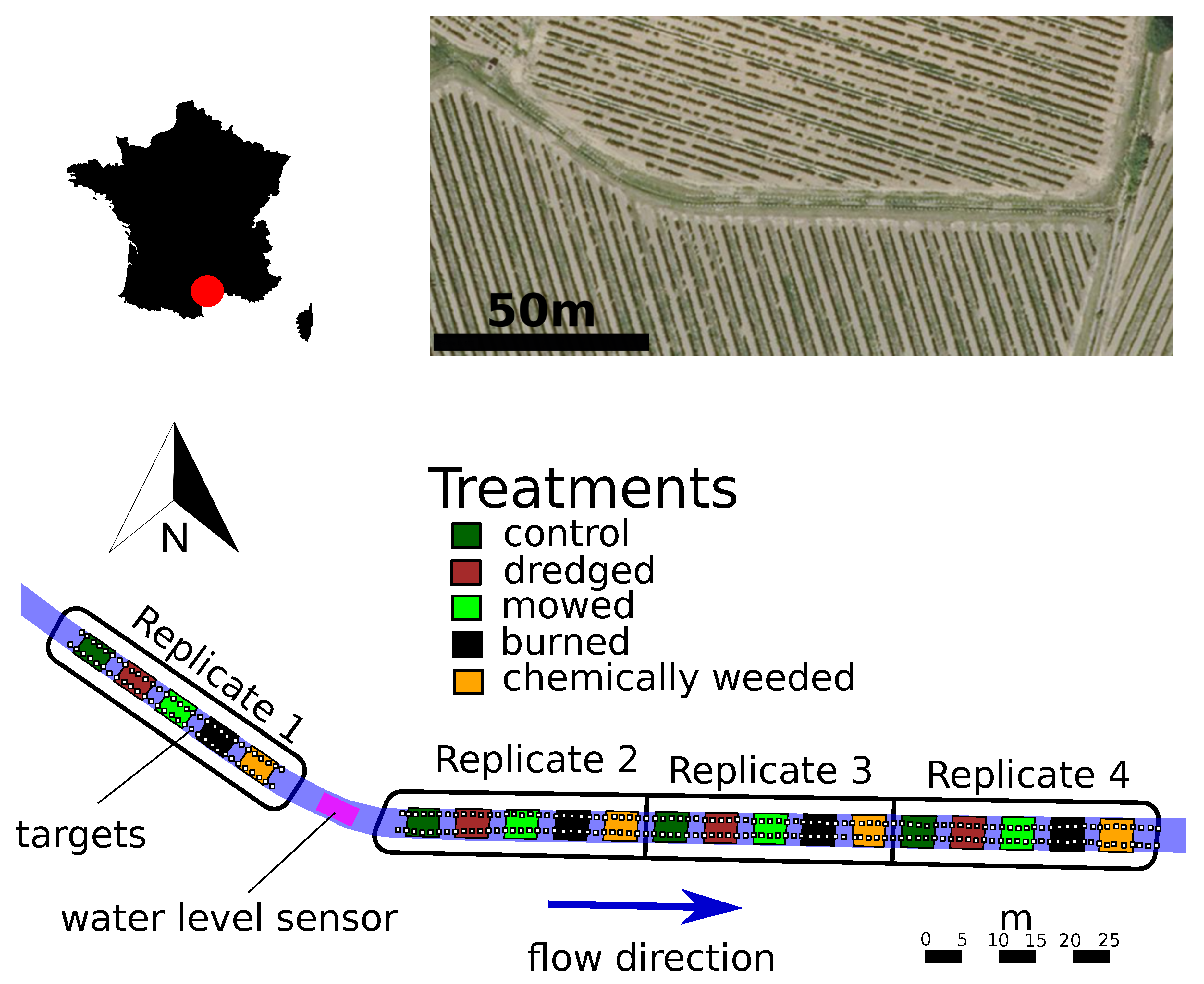
2.1. Study Site

The study was performed on a channel in a vineyard area located in southern France (43.48N, 3.34W). The climate is Mediterranean with scarce but heavy rainfall events generating intermittent flooding of the channel. The precipitation ranges from 600 to 800 mm per year, with a dry period from April to October and heavy rainfall in autumn and spring. The mean annual temperature is 14 °C [45].
The channel is part of a man-made network consisting of agricultural and roadside channels used to regulate excess overland water fluxes [3]. This channel has a 120-m length and a 3.3‰ bottom slope. Its cross-sections have a trapezoidal shape with a 60-cm depth, 60-cm bottom width and 160-cm top width.
An exhaustive characterization of channel species in April 2015 revealed an important diversity of plants with a richness similar to that observed in other channels located in the same geomorphological context [46]. The channel vegetation was mainly composed of Asteraceae and Poaceae species, with the latter being primarily located on the banks of the channel.
The water level inside the channel after rainfall events was monitored with a capacity sensor with centimetric precision [47]. Rainfall, temperature, wind velocity, and global radiation were measured by a meteorological station located 1.5 km from the study site.

2.2. Experimental Design and Maintenance Practices

The experimental design has been described in detail in [15]. In brief, five treatments were applied from upstream to downstream in 4-m-long quadrats separated by 2-m-long unmanaged buffers: (1) non-managed (control), (2) dredged, (3) mowed, (4) burned, and (5) chemically weeded (Figure 1). Each block was replicated four times according to a factorial design.
Dredging was performed using a straight spade to remove a 10-cm layer of dredged material from both the bottom and the sides of the channel. The channel was mowed using a brush cutter. Burning was performed by adding a fine layer of hay to help establish the fire. Finally, chemical weeding was implemented by a hand sprayer with glyphosate.

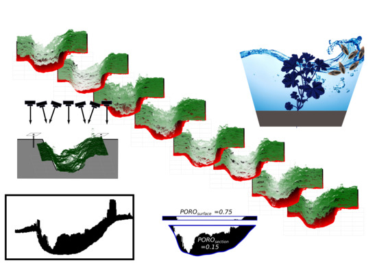
2.3. Applying the Ultra-Fine SfM-MVS Approach at the Study Site

The study was performed between April 2015 and July 2017 for a total of 35 surveys. Surveys were conducted monthly, except when maintenance practices were performed on some of the channel sections. In these cases, two surveys were made: on the day prior to and on the day after the maintenance practice. At the end of the study, the channel was completely burned to produce the digital terrain model (DTM) of the zone, i.e., the equivalent of the digital surface model (DSM) without vegetation cover.
In our study, the reproducibility of the procedure was analyzed by choosing a sufficient number of ground control points (GCPs) to ensure image alignment for a given survey and to help align all the surveys in the same spatial reference system [48]. GCPs consisted of vertical stakes with a 50-cm length buried 30 cm into the ground and topped with horizontal targets. The targets were rigid plastic squares with 10-cm edges coded in 16 bits, allowing approximately 2000 unique combinations of numbers. The planimetric and vertical positions of each target’s center were measured at the beginning of the study using a differential global positioning system (DGPS) at a 1-cm accuracy in the RGF93 system (EPSG:2154). The GCPs were regularly placed along both sides of the channel, 1 m from each other. This spacing between GCPs was selected to allow at least three targets to be included in a given image to help alignment using the SfM-MVS approach [29,49]. The GCPs were kept in place throughout the study period.
During the entire procedure, the camera was fixed on a 250-cm pole operated in continuous shooting mode using a Phottix© remote (Hong-Kong, China). Our protocol presents much similarities with the one used by ([37], Figure 3a), with the difference that we only used one single camera, which supposedly allows for better lens calibration conditions. We chose a time-lapse interval between images and operator walking speed ensuring a 90% overlap between successive images. Image data were acquired using a Nikon D3200 camera (Melville, NY, USA) with a fixed 28-mm AF Nikkor objective to obtain a resolution of ground pixels below 1 mm and a ground footprint of approximately 4 m2. The objective was set to infinity, and the camera was set in bulk mode to limit blurry images.
Because the approach was designed for high vegetation cover in a sharp channel, we considered both vertical and oblique perspectives to cope with occlusion effects due to complex canopies [35]. Both oblique and vertical imagery were acquired with the equipment described above and with a targeted 90% overlap. Oblique images were simply acquired by tilting the pole to the desired angle. Each channel section of approximately 30 m was surveyed in seven passages, with three passages acquired at the nadir of the two sides and the bottom of the channel and four passages converging towards the top of each bank (around −30° and 30° from the nadir, Figure 2). The three nadir image sets served as connectors of the four convergent image sets. Lower numbers of passages with different orientations were tested, with the undesirable consequence of a lower number of aligned images (data not shown). The survey was carried out around midday to limit hill shading and lasted for approximately one hour. Between 3500 and 4000 images were taken for each data acquisition survey, with an intensity of 30 images·m−1.

2.4. SfM-MVS Processing Chain for Generating the DTM, DSM and Orthophotos

Each set of images was processed for SfM-MVS modelling using Photoscan Pro© (v 1.2.6) (Agisoft LLC, St. Petersburg, Russia), given its efficiency compared to other software [35]. With Photoscan Pro©, targets were automatically recognized in the images (Figure 3). Sparse cloud processing was undertaken using the highest quality settings. After optimization of the sparse cloud, the dense cloud was reconstructed using medium and aggressive parameters to accelerate the processing time. Then, the dense cloud was meshed with the highest level, i.e., a number of vertexes corresponding to the number of points in the dense cloud. The complete parameter set used for the analysis is presented in Table 1. Analyses were performed on a high-performance computer (Intel© Xeon©, 40 cores, 128 GB RAM, NVIDIA Quadro K4200, Santa Clara, CA, USA), and each set of images took approximately 30 h to be fully processed. The final product of the SfM-MVS processing chain was a DSM at 1-cm resolution, a value that allows for reasonable computing time while keeping a proper representation of the canopy relatively to its spatial variability (more details given in the next section). The DSM from the last survey obtained after the complete burning of the channel was assimilated into a DTM given the absence of a vegetation cover.
The quality of the DSM was assessed by calculating the root mean square error (RMSE, in pixels) of the image alignment parameters to check the internal coherence of the image block-estimated geometries. The mean absolute error (MAE) between target simulated and observed positions was also calculated using a k-fold cross-validation procedure with k = 4. Within this procedure, a quarter of the positions were used for a validation test, and the remaining three quarters were used to fit the point cloud using solid transformation, i.e., with only rotation and translation of the cloud. The procedure was repeated four times until all targets were included in the training and testing datasets. Then, the four sets of results were averaged to produce a single estimate per survey. Quality indicators of the DSM (RMSE, MAE) were related to meteorological data using Pearson product-moment correlation.

2.5. Estimation of Indicator of Porosity

To obtain the vegetation point clouds, the DSMs and the DTMs were transformed into point clouds and cropped according to the limit of each quadrat. Each cropped DSM was shifted and toggled considering the slope of the channel to be perpendicular to the cross-section. We applied the same procedure to the DTM. Then, we filled the volume below each DSM with regularly sampled points to simulate the vegetation cover below the canopy (Figure 4). The periodicity of canopy height variation having been estimated at approximately 5 cm through a 2D fast-fourier transform, the point spacing was fixed to 1 cm, a value which gives a reasonable security margin relatively to the theoretical requested value given by the Shannon sampling theorem [50] without a significant increase in computing time.
The mean vegetation height was calculated by substracting the DSM from the DTM and averaging the difference over the entire quadrat. Quality indicators of the DSM (RMSE, MAE) were related to vegetation height using Pearson product-moment correlation. Temporal effect of treatment on vegetation height was estimated using a one-way ANOVA applied on each date with treatment as explaining variable of vegetation height, the latter being normally distributed (Shapiro–Wilk test >0.05 for all dates). Difference among means were analyzed with Tukey’s honestly significant difference (HSD) test on the ANOVA model.
To calculate the indicators of porosity, we followed the approach of [23] by projecting the vegetation clouds in the direction of flow from each quadrat on the channel section to obtain an unique indicator of porosity for each quadrat. The projection of the cloud consisted of a raster with values ranging between 0 and 1 (Figure 4). We kept the best relationship found in [23] by filling the raster values below the canopy of the raster (Figure 4). The values of the raster that were strictly positive were transformed to 1 (Figure 4). The corresponding raster, averaged over the whole section, is referred to as P O R O s e c t i o n (Figure 4). This raster ranges from 0 (absence of porosity) to 1 (total porosity).
In the same way, we calculated another parameter to link seed retention to emergent vegetation. We started from the binarized and filled raster corresponding to the projection of the vegetation cloud, and we then sliced it around the water surface as an indicator of the seed retention due to obstacles provided by protruding vegetation. We based our assumption on the work done by [51] on floating particle trapping, where the authors assumed that the particle trapping probability is linked to the spacing between adjacent plants. This indicator, P O R O s u r f a c e , corresponded to the raster slice averaged over the width of the water surface. Similarly to P O R O s e c t i o n , P O R O s u r f a c e ranges from 0 (absence of porosity) to 1 (total porosity) (Figure 4).
We virtually filled each quadrat with water from the bottom (DTM) to the highest virtual water level corresponding to the overflow limit (Figure 4). For each filling level, we considered the polygon depicting the vertical section of the channel, and we calculated, for each combination of water level × time and for each treatment, the indicators of porosity P O R O s e c t i o n and P O R O s u r f a c e . Temporal effect of treatment on porosities were estimated using a one-way ANOVA applied on each date with treatment as explaining variable of porosities, the latter being normally distributed (Shapiro-Wilk test > 0.05). Difference among means were analyzed with Tukey’s HSD test. Difference between P O R O s e c t i o n and P O R O s u r f a c e was tested using a Generalized Linear Model (GLM) with binomial distribution. Values of the indicators were averaged over the four replicates.

2.6. Manipulation of Time Series

Considering the high volume of data produced (i.e., approximately 150,000 images were taken and processed), post-processing algorithms were specifically designed for reproducibility of the treatments. Target detection, image alignment, point cloud, DSM generation and cross-validation procedures were automated using the Python scripting console provided in Photoscan Pro©. Point cloud post-processing, i.e., cropping and shifting, was performed using CloudCompare [52] called recursively for each quadrat by R software (3.5.1, Vienna, Austria) [53]. Point clouds were manipulated using R software with a specific package called data.table used for high-speed calculation performed on large datasets. Statistical analyses were conducted using R software [53].

3. Results

3.1. Quality of DSM and DTM Reconstructions

Choosing a high intensity level helped improve alignment accuracy for all surveys, with the alignment proportion always reaching nearly 100%. The RMSE was approximately 1 ± 0.5 pixels. The MAE was 0.05 ± 0.03 m on average for all surveys. Moreover, the evolution of vegetation height during the period was related to neither the RMSE nor the MAE (Pearson product-moment correlation < 0.6), suggesting that the vegetation cover outside the zone disturbed by management practices, remaining rather constant in terms of configuration and development between surveys, was the main factor affecting the RMSE and MAE. This permanent cover partially masked some of the ground control points for oblique view acquisition.
Wind velocities averaged 22 km·h−1 over the surveys, with peaks at 40 km·h−1 for three surveys. Two surveys were carried out under rainy conditions. The global radiation averaged 217 joules·cm−2 during the surveys, with two surveys performed under low-illumination conditions, i.e., global radiation under 50 joules·cm−2. The RMSE and MAE were not related to wind velocity, global radiation or rainfall over the survey duration (Pearson product-moment correlation < 0.6).

3.2. Evolution of the Porosity Indicators

Regarding the evolution of water level fluctuations during the study period, the channel experienced eight major flooding events, with the water level peaking from 10 to 60 cm. The channel bottom was lastingly submerged during two periods: in spring 2015 and 2017. We observed an exceptionally dry period in spring 2016 with consequences for vegetation height in all treatments.
Figure 5 illustrates the yearly evolution of vegetation height across practices. Logically, the height of vegetation cover was higher for the control than for the other management practices (p < 0.05 in all cases, Tukey’s HSD), with fluctuations in height related to seasons. The evolution of vegetation cover for the other treatments was more associated with the timing of maintenance than with seasonal effects. The control treatment exhibited a diminution of vegetation height just after the major flow event that occurred in December 2016. The vegetation of the dredged section required only one year to recover to the same height observed in the control (p < 0.05 before April 2016 then p > 0.05 after April 2016, Tukey’s HSD). According to the maintenance schedule, the vegetation height in the burned and mowed sections exhibited non-phased variations, with a reduction in vegetation cover in winter for the burned treatment and in summer for the mowed treatment, in comparison to the control (p < 0.05, Tukey’s HSD). Finally, the chemically weeded treatment tended to limit variations in the vegetation height, always under the control (p < 0.05 for 30% of the dates, Tukey’s HSD), with the dead vegetation from the treatment being progressively replaced by new stands in spring.
Figure 6 presents examples of DTM and DSM point clouds during the growing season. At the scale of a quadrat, we distinguished heterogeneity in vegetation height along the cross-section of the channel. The two sides of the channel presented a stable vegetation height across the surveys and the treatments (Figure 2). The bottom and bank parts of the channel contained an important and homogeneous vegetation cover in the chemically weeded and control treatments, with the depth of the cover exceeding the depth of the channel for the latter treatment. In contrast to the mowed and burned treatments, which exhibited high variations in cover during the surveys, the control and chemically weeded treatments exhibited cover that remained stable during the study period. The vegetation cover grew preferentially on the banks of the dredged channel, with a lower growth rate during the study period in these treatments than in the mowed and burned treatments.
Figure 7 presents the contour plots of the indicators of porosities ( P O R O s e c t i o n in Figure 7a and P O R O s u r f a c e in Figure 7b), with time on the abscissa and the virtual water level on the ordinate, for each treatment. Regarding the timing of the eight major flow events, only the mowed treatment was phased with the peak flow, leading to the highest porosities. The P O R O s u r f a c e indicator was high for the major flow events occurring in autumn 2016, i.e., when the virtual water level was above 50 cm, but only for the mowed and chemically weeded treatments, suggesting a higher temporal efficiency of these treatments in comparison to the others.
According to Figure 8, the P O R O s e c t i o n and P O R O s u r f a c e at the highest virtual water level reached a peak of between 0.7 and 0.8 for the mowed and burned treatments. The porosity at the surface, P O R O s u r f a c e , presented significantly higher values than that for P O R O s e c t i o n (binomial GLM, p < 0.001). Among the treatments, the control treatment showed the lowest P O R O s e c t i o n and P O R O s u r f a c e values, i.e., the lowest permeability to water flow and seeds, during the study period, in comparison to the other treatments (p < 0.05, Tukey’s HSD). The mowing helped maintain a low vegetation cover throughout the year and, consequently, high porosity for the highest virtual water level in comparison to the control (p < 0.05, Tukey’s HSD). Porosities reached the control level three months on average after applying the treatment for all treatments (p < 0.05, Tukey’s HSD); then, no significant differences were measured between treatment and control.

4. Discussion

The elaboration of a diachronic series of DSMs at ultra-fine resolution required an automated processing chain to handle the large amount of data generated by the surveys. The need for process automation has already been expressed by [32] for future development of the SfM-MVS approach and was diagnosed by [24] as an disadvantage to actual repeatability. Through Python scripting and batch processing, Photoscan Pro© software allowed for accessing a full range of automated post-processing options, unlike other software such as Photosynth (2.0, University of Washington, WA, USA) and 123D Catch (3.0, Autodesk, San Rafael, CA, USA) [30], making multi-temporal applications of the SfM-MVS approach over long time periods possible. Furthermore, R software is particularly interesting for its ability to recursively call the full set of software dedicated to point cloud post-processing and large dataset handling. To the best of our knowledge, this is the first time that R software was tested in an automated processing chain for SfM-MVS post-processing.
The SfM-MVS technique used in this study provides access to vegetation characteristics with a higher accuracy than that of other manual surveys [15] but requires preparation of the survey area. The two indicators of porosities could not be measured visually in the field because they are based on fine monitoring of vegetation cover and channel topography. The channel should be accessible by foot, bordered by a high density of ground control markers, and not exceed several hundreds of metres. In comparison to unmanned aerial vehicle (UAVs) used for image acquisition, the use of a pole enabled the surveys to be performed under windy conditions with low illumination and significant rainfall amounts. The same conditions would be prohibitive for wind-sensitive UAVs [25]. The absence of correlations of the RMSE and MAE with the climatic conditions confirms the robustness of the method for performing surveys under various climatic conditions.
The survey intensity considered in our approach is within the range of frequencies used in other SfM-MVS studies focusing on gully erosion (between 4.4 and 64.3 images·m−1, cf [37]). A survey duration of one hour exceeds the maximal limit of 30 min proposed by [54] to limit shadow changes and the associated flawed image matching, but, in our case, the linear progression of the observer along the channel resulted in a lower actual time difference between overlapping images. This is supported by the fact that we almost reached 100% matching for all surveys. It is also interesting to note that, contrarily to what is often admitted (e.g., by [28]), the use of a rigorous survey protocol led to acquisition times that would probably be comparable or even better than acquisition times with multi-station TLS. In addition, the geometry of agricultural waterways—a steep incision in the relatively flat surrounding cultivated areas—would require either a significant number of stations for TLS or the use of low-altitude airborne laser scanning.
Choosing a robust remote sensing method to obtain complete coverage of a vegetated channel necessitated a high survey intensity with a medium alignment quality and an average error larger than those for other studies on relatively flat surfaces with limited vegetation [33,34,35]. Specifically, the absolute error calculated from ground control points was slightly higher than that for studies on gully erosion (on the basis of average errors between 0.03 and 0.07 m gathered in [37]). Because these studies focused on ground measures, the proportion of vegetation was considerably lower than that in our study and could explain this difference in error. Based on the MAE, our approach obtained better results than that used in olive tree plantations in [34] (0.46 m) and dryland trees in [35] (0.07 m), but poorer results than that used in maize and sorghum in [33] (0.03 m). We could not compare our results to those from the study of [36] because they compared only vegetation properties determined with an SfM-MVS method without ground control points.
The porosities could be underestimated because they were based on vegetation clouds under dry conditions, while water flows induced spatial plant reconfiguration that is known to limit resistance factors [55]. Filling the areas below the vegetation canopy should lead to an underestimation of the porosities, depending on the vertical heterogeneity in the plant architecture. However, this effect could be counterbalanced by the presence of small plants below the canopy. For example, the decrease in vegetation height occurring in December 2016 suggests a washing out of the dead vegetation [15,56] and a probable reconfiguration of vegetation due to the flow [57]. It is worth mentioning that the vegetation height estimated with our method showed lower error (0.1 m) across treatments and surveys than that in the study of [15] (0.2 m), confirming the robustness of the SfM-MVS surveys for vegetation monitoring.
Applying all management practices greatly decreased the water resistance but with a recovery time sometimes too quick to have an impact during flow periods. Dredging, initially used to remove sediment layers, could negatively impact the seed bank inside the channel. It may also remove superficial roots, increasing the effective shear stress at the bottom of the channel [58]. However, the recovery of vegetation one year after dredging suggests that a maintenance interval for this practice of five years [14] is insufficient to have a mid-term impact on vegetation cover. This result is particularly true for burning out of step with the rainy period. Considering the major flow events during the period, it appears that mowing and burning have opposite effects on vegetation porosity at the surface, with the first contributing to seed dispersal and the other enhancing seed retention. Mowing the vegetation seemed to be the only treatment able to maintain a high porosity at the surface during the major flow events, regardless of the water level. Mowing, by increasing the amount of dead vegetation inside the channel, could also reduce the effective shear stress [59]. This practice also increases species richness throughout the landscape via the dispersal of floating seeds of riparian plant species [60]. Inversely, from the perspective of capturing the maximal amount of weed seeds, burning the vegetation in winter seems to be adequate. This practice helps limit the spread of weeds in agricultural landscapes.

5. Conclusions

The application of frequent monitoring of vegetation growth according to agricultural practices has never been studied in agricultural waterways, despite the critical positions of these waterways at the interface between agricultural plots. Frequent monitoring of the vegetation cover in agricultural waterways is necessary because the waterways experience high variations throughout the year due to the schedule of management practices, the intermittency of water flow depending on rainfall events, and the seasonality of vegetation regrowth. Combining time series of vegetation characteristics is the only way to estimate the critical period for maximizing the efficiency of agricultural practices because, as highlighted by this study, several practices are out of phase with the flow periods.
The use of the SfM-MVS approach has proven its value in their particular conditions. Combined with an automated processing chain for dense cloud construction and post-processing, it paves the way to a systematic processing of time series of vegetation monitoring. This study also highlighted recommendations in using the SfM-MVS approach at a very high resolution over dense time series. To increase the robustness of the surveys, the areas must be densely covered by ground control points, and the intensity of image capture during surveys must be high to facilitate image matching and co-registration of multi-temporal digital surface models. Future research should be oriented towards new methodologies capable of limiting the cumbersome implementation of remote sensing projects in the field.

Author Contributions

Conceptualization, F.V. and J.-S.B. and J.D.; Methodology, F.V. and D.F.; Software, F.V. and D.F.; Formal Analysis, F.V.; Writing—Original Draft Preparation, F.V.; Writing—Review and Editing, J.D. and G.R. and D.F. and G.B. and J.-S.B.; Visualization, F.V.; Funding Acquisition, F.V.

Funding

The authors are grateful to the INRA, who funded the experimental work presented in this paper within the Pari-Scientifique: Hydro-ecologie des fosses agricoles project (INRA-EA). This project is also supported by the Agropolis Fondation under the reference ID 1605-034 through the Investissements d’avenir programme (Labex Agro: ANR-10-LABX-0001-01).

Acknowledgments

The authors are very grateful to the LISAH laboratory’s technicians and especially Sebastien Troiano for his valuable support and involvement in the collection of the data and the preparation of the targets. The authors thank the two farmers, namely, Mr Cros and Mr Boulade, who authorized the experiments in their fields.

Conflicts of Interest

The authors declare no conflict of interest.

Abbreviations

The following abbreviations are used in this manuscript:
DEMDigital Elevation Model
DSMDigital Surface Model
DTMDigital Terrain Model
GLMGeneralized Linear Model
HSDHonestly Significant Difference
MAEMean Absolute Error (in m)
RMSERoot Mean Squared Error (in m)
SfM-MVSStructure-from-Motion approach using a Multi-View Stereo algorithm
TLSTerrestrial Laser Scanner
UAVUnmanned Aerial Vehicle

References

  1. Herzon, I.; Helenius, J. Agricultural drainage ditches, their biological importance and functioning. Biol. Conserv. 2008, 141, 1171–1183. [Google Scholar] [CrossRef]
  2. Pierce, S.; Kröger, R.; Pezeshki, R. Managing Artificially Drained Low-Gradient Agricultural Headwaters for Enhanced Ecosystem Functions. Biology 2012, 1, 794–856. [Google Scholar] [CrossRef] [PubMed]
  3. Dollinger, J.; Dagès, C.; Bailly, J.S.; Lagacherie, P.; Voltz, M. Managing ditches for agroecological engineering of landscape. A review. Agron. Sustain. Dev. 2015, 35, 999–1020. [Google Scholar] [CrossRef] [Green Version]
  4. Curran, J.C.; Hession, W.C. Vegetative impacts on hydraulics and sediment processes across the fluvial system. J. Hydrol. 2013, 505, 364–376. [Google Scholar] [CrossRef]
  5. Nicholls, C.I.; Parrella, M.; Altieri, M.A. The effects of a vegetational corridor on the abundance and dispersal of insect biodiversity within a northern California organic vineyard. Landsc. Ecol. 2001, 16, 133–146. [Google Scholar] [CrossRef]
  6. Forman, R.T.; Baudry, J. Hedgerows and hedgerow networks in landscape ecology. Environ. Manag. 1984, 8, 495–510. [Google Scholar] [CrossRef]
  7. Armitage, P.D.; Szoszkiewicz, K.; Blackburn, J.H.; Nesbitt, I. Ditch communities: A major contributor to floodplain biodiversity. Aquat. Conserv. Mar. Freshw. Ecosyst. 2003, 13, 165–185. [Google Scholar] [CrossRef]
  8. Davies, B.; Biggs, J.; Williams, P.; Whitfield, M.; Nicolet, P.; Sear, D.; Bray, S.; Maund, S. Comparative biodiversity of aquatic habitats in the European agricultural landscape. Agric. Ecosyst. Environ. 2008, 125, 1–8. [Google Scholar] [CrossRef]
  9. Johansson, M.E.; Nilsson, C.; Nilsson, E. Do rivers function as corridors for plant dispersal? J. Veg. Sci. 1996, 7, 593–598. [Google Scholar] [CrossRef]
  10. Nilsson, C.; Brown, R.L.; Jansson, R.; Merritt, D.M. The role of hydrochory in structuring riparian and Wetland vegetation. Biol. Rev. 2010, 85, 837–858. [Google Scholar] [CrossRef] [PubMed]
  11. Nepf, H.M. Hydrodynamics of vegetated channels. J. Hydraul. Res. 2012, 50, 262–279. [Google Scholar] [CrossRef] [Green Version]
  12. Järvelä, J. Determination of flow resistance caused by non-submerged woody vegetation. Int. J. River Basin Manag. 2004, 2, 61–70. [Google Scholar] [CrossRef]
  13. Lecce, S.A.; Pease, P.P.; Gares, P.A.; Wang, J. Seasonal controls on sediment delivery in a small coastal plain watershed, North Carolina, USA. Geomorphology 2006, 73, 246–260. [Google Scholar] [CrossRef]
  14. Levavasseur, F.; Biarnès, A.; Bailly, J.S.; Lagacherie, P. Time-varying impacts of different management regimes on vegetation cover in agricultural ditches. Agric. Water Manag. 2014, 140, 14–19. [Google Scholar] [CrossRef]
  15. Dollinger, J.; Vinatier, F.; Voltz, M.; Dagès, C.; Bailly, J.S. Impact of maintenance operations on the seasonal evolution of ditch properties and functions. Agric. Water Manag. 2017, 193, 191–204. [Google Scholar] [CrossRef] [Green Version]
  16. Sabbatini, M.; Murphy, K.; Irigoyen, J. Vegetation–environment relationships in irrigation channel systems of southern Argentina. Aquat. Bot. 1998, 60, 119–133. [Google Scholar] [CrossRef]
  17. Malaterre, P.O. Regulation of irrigation canals. Irrig. Drain. Syst. 1995, 9, 297–327. [Google Scholar] [CrossRef]
  18. Rubol, S.; Ling, B.; Battiato, I. Universal scaling-law for flow resistance over canopies with complex morphology. Sci. Rep. 2018, 8, 4430. [Google Scholar] [CrossRef] [PubMed]
  19. Green, J.C. Modelling flow resistance in vegetated streams: Review and development of new theory. Hydrol. Process. 2005, 19, 1245–1259. [Google Scholar] [CrossRef]
  20. Defina, A.; Peruzzo, P. Floating particle trapping and diffusion in vegetated open channel flow. Water Resour. Res. 2010, 46, W11525. [Google Scholar] [CrossRef]
  21. Green, J.C. Comparison of blockage factors in modelling the resistance of channels containing submerged macrophytes. River Res. Appl. 2005, 21, 671–686. [Google Scholar] [CrossRef]
  22. Friedli, M.; Kirchgessner, N.; Grieder, C.; Liebisch, F.; Mannale, M.; Walter, A. Terrestrial 3D laser scanning to track the increase in canopy height of both monocot and dicot crop species under field conditions. Plant Methods 2016, 12, 9. [Google Scholar] [CrossRef] [PubMed]
  23. Vinatier, F.; Bailly, J.S.; Belaud, G. From 3D grassy vegetation point cloud to hydraulic resistance: Application to close-range estimation of Manning coefficients for intermittent open channels. Ecohydrology 2017, 10, e1885. [Google Scholar] [CrossRef] [Green Version]
  24. Boothroyd, R. Flow-Vegetation Interactions at the Plant-Scale: The Importance of Volumetric Canopy Morphology on Flow Field Dynamics. Ph.D. Thesis, Durham University, Durham, UK, 6 November 2017. [Google Scholar]
  25. Verhoeven, G.J. Providing an archaeological bird’s-eye view—An overall pictureof ground-based meansto execute low-altitude aerial photography (LAAP) in archaeology. Archaeol. Prospect. 2009, 16, 233–249. [Google Scholar] [CrossRef]
  26. Rose, J.C.; Kicherer, A.; Wieland, M.; Klingbeil, L.; Töpfer, R.; Kuhlmann, H. Towards automated large-scale 3D phenotyping of vineyards under field conditions. Sensors 2016, 16, 2136. [Google Scholar] [CrossRef] [PubMed]
  27. Paulus, S.; Behmann, J.; Mahlein, A.K.; Plümer, L.; Kuhlmann, H. Low-cost 3D systems: Suitable tools for plant phenotyping. Sensors 2014, 14, 3001–3018. [Google Scholar] [CrossRef] [PubMed]
  28. Chandler, J.H.; Buckley, S.J. Structure from motion (SFM) photogrammetry vs. terrestrial laser scanning. In Geoscience Handbook 2016: AGI Data Sheets, 5th ed.; American Geosciences Institute: Alexandria, VA, USA, 2016; pp. 1–4. [Google Scholar]
  29. James, M.R.; Robson, S. Straightforward reconstruction of 3D surfaces and topography with a camera: Accuracy and geoscience application. J. Geophys. Res. Earth Surf. 2012, 117, 1–17. [Google Scholar] [CrossRef]
  30. Smith, M.W.; Carrivick, J.L.; Quincey, D.J. Structure from motion photogrammetry in physical geography. Prog. Phys. Geogr. 2015, 40, 247–275. [Google Scholar] [CrossRef] [Green Version]
  31. Carrivick, J.; Smith, M.; Quincey, D. Structure from Motion in the Geosciences; Wiley: Hoboken, NJ, USA, 2016; p. 208. [Google Scholar]
  32. Eltner, A.; Kaiser, A.; Castillo, C.; Rock, G.; Neugirg, F.; Abellán, A. Image-based surface reconstruction in geomorphometry-merits, limits and developments. Earth Surf. Dyn. 2016, 4, 359–389. [Google Scholar] [CrossRef]
  33. Malambo, L.; Popescu, S.C.; Murray, S.C.; Putman, E.; Pugh, N.A.; Horne, D.W.; Richardson, G.; Sheridan, R.; Rooney, W.L.; Avant, R.; et al. Multitemporal field-based plant height estimation using 3D point clouds generated from small unmanned aerial systems high-resolution imagery. Int. J. Appl. Earth Obs. Geoinf. 2018, 64, 31–42. [Google Scholar] [CrossRef]
  34. Díaz-Varela, R.A.; de la Rosa, R.; León, L.; Zarco-Tejada, P.J. High-resolution airborne UAV imagery to assess olive tree crown parameters using 3D photo reconstruction: Application in breeding trials. Remote Sens. 2015, 7, 4213–4232. [Google Scholar] [CrossRef]
  35. Cunliffe, A.M.; Brazier, R.E.; Anderson, K. Ultra-fine grain landscape-scale quantification of dryland vegetation structure with drone-acquired structure-from-motion photogrammetry. Remote Sens. Environ. 2016, 183, 129–143. [Google Scholar] [CrossRef] [Green Version]
  36. Gillan, J.K.; Karl, J.W.; Duniway, M.; Elaksher, A. Modeling vegetation heights from high resolution stereo aerial photography: An application for broad-scale rangeland monitoring. J. Environ. Manag. 2014, 144, 226–235. [Google Scholar] [CrossRef] [PubMed]
  37. Castillo, C.; James, M.R.; Redel-Macías, M.D.; Pérez, R.; Gómez, J.A. SF3M software: 3D photo-reconstruction for non-expert users and its application to a gully network. Soil 2015, 1, 583–594. [Google Scholar] [CrossRef]
  38. Kaiser, A.; Neugirg, F.; Rock, G.; Müller, C.; Haas, F.; Ries, J.; Schmidt, J. Small-scale surface reconstruction and volume calculation of soil erosion in complex moroccan Gully morphology using structure from motion. Remote Sens. 2014, 6, 7050–7080. [Google Scholar] [CrossRef]
  39. Feurer, D.; Planchon, O.; El Maaoui, M.A.; Ben Slimane, A.; Boussema, M.R.; Pierrot-Deseilligny, M.; Raclot, D. Using kites for 3D mapping of gullies at decimetre-resolution over several square kilometres: A case study on the Kamech catchment, Tunisia. Nat. Hazards Earth Syst. Sci. 2018, 18, 1567–1582. [Google Scholar] [CrossRef]
  40. Javernick, L.; Brasington, J.; Caruso, B. Modeling the topography of shallow braided rivers using Structure-from-Motion photogrammetry. Geomorphology 2014, 213, 166–182. [Google Scholar] [CrossRef]
  41. Javernick, L.; Hicks, D.M.; Measures, R.; Caruso, B.; Brasington, J. Numerical Modelling of Braided Rivers with Structure-from-Motion-Derived Terrain Models. River Res. Appl. 2016, 32, 1071–1081. [Google Scholar] [CrossRef]
  42. Woodget, A.S.; Carbonneau, P.E.; Visser, F.; Maddock, I.P. Quantifying submerged fluvial topography using hyperspatial resolution UAS imagery and structure from motion photogrammetry. Earth Surf. Process. Landf. 2015, 40, 47–64. [Google Scholar] [CrossRef]
  43. Dietrich, J.T. Riverscape mapping with helicopter-based Structure-from-Motion photogrammetry. Geomorphology 2016, 252, 144–157. [Google Scholar] [CrossRef]
  44. Casado, M.; Gonzalez, R.; Kriechbaumer, T.; Veal, A.; Casado, M.R.; Gonzalez, R.B.; Kriechbaumer, T.; Veal, A. Automated Identification of River Hydromorphological Features Using UAV High Resolution Aerial Imagery. Sensors 2015, 15, 27969–27989. [Google Scholar] [CrossRef] [PubMed] [Green Version]
  45. Levavasseur, F.; Bailly, J.S.; Lagacherie, P.; Colin, F.; Rabotin, M. Simulating the effects of spatial configurations of agricultural ditch drainage networks on surface runoff from agricultural catchments. Hydrol. Process. 2012, 26, 3393–3404. [Google Scholar] [CrossRef] [Green Version]
  46. Rudi, G.; Bailly, J.S.; Vinatier, F. Using geomorphological variables to predict the spatial distribution of plant species in agricultural drainage networks. PLoS ONE 2018, 13, e0191397. [Google Scholar] [CrossRef] [PubMed]
  47. Crabit, A.; Colin, F.; Bailly, J.S.; Ayroles, H.; Garnier, F. Soft water level sensors for characterizing the hydrological behaviour of agricultural catchments. Sensors 2011, 11, 4656–4673. [Google Scholar] [CrossRef] [PubMed]
  48. James, L.A.; Hodgson, M.E.; Ghoshal, S.; Latiolais, M.M. Geomorphic change detection using historic maps and DEM differencing: The temporal dimension of geospatial analysis. Geomorphology 2012, 137, 181–198. [Google Scholar] [CrossRef]
  49. Kraus, K.; Waldhäusl, P.; Grussenmeyer, P.; Reis, O. Manuel de Photogrammétrie: Principes et Procédés Fondamentaux; Hermès Science Publications: Paris, France, 1997; p. 407. [Google Scholar]
  50. Jerri, A. The Shannon sampling theorem—Its various extensions and applications: A tutorial review. Proc. IEEE 1977, 65, 1565–1596. [Google Scholar] [CrossRef]
  51. Peruzzo, P.; Defina, A.; Nepf, H. Capillary trapping of buoyant particles within regions of emergent vegetation. Water Resour. Res. 2012, 48, W07512. [Google Scholar] [CrossRef]
  52. Girardeau-Montaut, D. CloudCompare: 3D Point Cloud and Mesh Processing Software. Available online: https://www.danielgm.net/cc/ (accessed on 1 October 2018).
  53. The R Core Team. R: A Language and Environment for Statistical Computing; R Foundation for Statistical Computing: Vienna, Austria, 2018. [Google Scholar]
  54. Bemis, S.P.; Micklethwaite, S.; Turner, D.; James, M.R.; Akciz, S.; Thiele, S.T.; Bangash, H.A. Ground-based and UAV-Based photogrammetry: A multi-scale, high-resolution mapping tool for structural geology and paleoseismology. J. Struct. Geol. 2014, 69, 163–178. [Google Scholar] [CrossRef]
  55. Whittaker, P.; Wilson, C.; Aberle, J.; Rauch, H.P.; Xavier, P. A drag force model to incorporate the reconfiguration of full-scale riparian trees under hydrodynamic loading. J. Hydraul. Res. 2013, 51, 569–580. [Google Scholar] [CrossRef]
  56. Bennett, S.J.; Simon, A. Riparian Vegetation and Fluvial Geomorphology; American Geophysical Union: Washington, DC, USA, 2004; p. 282. [Google Scholar]
  57. Luhar, M.; Nepf, H.M. Flow-induced reconfiguration of buoyant and flexible aquatic vegetation. Limnol. Oceanogr. 2011, 56, 2003–2017. [Google Scholar] [CrossRef] [Green Version]
  58. Zhang, G.h.; Tang, K.m.; Ren, Z.p.; Zhang, X.C. Impact of Grass Root Mass Density on Soil Detachment Capacity by Concentrated Flow on Steep Slopes. Trans. ASABE 2013, 56, 927–934. [Google Scholar]
  59. Gyssels, G.; Poesen, J.; Bochet, E.; Li, Y. Impact of plant roots on the resistance of soils to erosion by water: A review. Prog. Phys. Geogr. 2005, 29, 189–217. [Google Scholar] [CrossRef]
  60. Jansson, R.; Zinko, U.; Merritt, D.M.; Nilsson, C. Hydrochory increases riparian plant species richness: A comparison between a free-flowing and a regulated river. J. Ecol. 2005, 93, 1094–1103. [Google Scholar] [CrossRef]
Figure 1. Location of the study site and sequence of maintenance practices. Positions of the control points are represented by white squares. Colored polygons represented the areas of each maintenance practice.
Remotesensing 10 02050 g001
Figure 2. Order of passages and orientation of the pole during SfM-MVS acquisition. The numbers from 1 to 7 in the upper part of the image stand for the order of passages of the cameras. Angles of the oblique imagery for the passages 2–3 and 6–7 are indicated, the passages 1, 4, 5 being realized in nadir.
Remotesensing 10 02050 g002
Figure 3. Illustration of automatic recognition of the targets on a picture using Photoscan Pro©. (a) original image; (b) image with recognized targets (boxes linked to a red dot).
Remotesensing 10 02050 g003
Figure 4. Illustration of the post-processing procedure of the DSM on a sub-sample of the zone corresponding to a control quadrat.
Remotesensing 10 02050 g004
Figure 5. Evolution of the mean difference between the DSM and the DTM across different treatments presented from top to bottom: control, dredged, mowed, burned, and chemically weeded. The dots correspond to the value averaged over the four replicates, and the vertical lines, to the standard deviation. Black arrows indicate the timing of the practice. The star symbol * indicated that treatment was significantly different from control at p < 0.05 (based on Tukey’s HSD).
Remotesensing 10 02050 g005
Figure 6. Time series of the point clouds showing the DTM (in black and red) and the DSM (in white and green) at a 1-cm resolution for four representative surveys in 2016 across different treatments presented in rows from top to bottom: control, dredged, mowed, burned, and chemically weeded. Black arrows indicate the timing of the practice.
Remotesensing 10 02050 g006
Figure 7. Dynamics of the vegetation indicators across different treatments presented in columns from left to right: control, dredged, mowed, burned, and chemically weeded. (a,b) from top to bottom, contour plots of the porosity indicators P O R O s e c t i o n and P O R O s u r f a c e against virtual water level on the ordinate and time on the abscissa. Values of porosities are between 0 (non-porous) and 1 (totally porous). Contour lines are drawn on the plots to better represent the variation in the indicators. The red dots represent the peaks of water levels for the main flow events during the study period. Vertical dashed lines delimit years. Black arrows indicate the timing of the practice.
Remotesensing 10 02050 g007
Figure 8. Evolution of the two indicators P O R O s e c t i o n (thick line) and P O R O s u r f a c e (fine line) against time and across different treatments presented from top to bottom: control, dredged, mowed, burned, and chemically weeded. The dots correspond to the value averaged over the four replicates, and the standard deviations were not represented for readability. The two indicators were estimated for a virtual water level of 0.5 m. Black arrows indicate the timing of the practice. The star symbol * indicated that treatment was significantly different from control at p < 0.05 (based on Tukey’s HSD).
Remotesensing 10 02050 g008
Table 1. Parameters used in PhotoScan Pro©.
Processing StepPropertyValue
AlignmentAccuracyHighest
Pair preselectionGeneric
Key point limit200,000
Tie point limit100,000
Adaptive camera model fittingYes
OptimizationLens parametersf,b1,b2,cex,cy
k1,k2,k3,k4,p1,p2
Marker accuracy (pix)0.1
Marker accuracy (m)0.01
Tie point accuracy (pix)0.1
Dense cloudQualityMedium
Depth filteringAggressive
MeshSurface typeCustom
InterpolationDisabled
QualityMedium
Depth filteringModerate
DEMPixel size (m)0.01

