Article

Identifying Mangrove Species Using Field Close-Range Snapshot Hyperspectral Imaging and Machine-Learning Techniques

1
Guangdong Provincial Engineering Research Center for Public Security and Disaster, Guangdong Key Laboratory for Urbanization and Geo-simulation, School of Geography and Planning, Sun Yat-sen University, Guangzhou 510275, China
2
Center of GeoInformatics for Public Security, School of Geographic Sciences, Guangzhou University, Guangzhou 510006, China
3
Department of Geography, University of Cincinnati, Cincinnati, OH 45221-0131, USA
*
Authors to whom correspondence should be addressed.
Remote Sens. 2018, 10(12), 2047; https://doi.org/10.3390/rs10122047
Submission received: 25 October 2018 / Revised: 11 December 2018 / Accepted: 14 December 2018 / Published: 16 December 2018

Abstract

:
Investigating mangrove species composition is a basic and important topic in wetland management and conservation. This study aims to explore the potential of close-range hyperspectral imaging with a snapshot hyperspectral sensor for identifying mangrove species under field conditions. Specifically, we assessed the data pre-processing and transformation, waveband selection and machine-learning techniques to develop an optimal classification scheme for eight mangrove species in Qi’ao Island of Zhuhai, Guangdong, China. After data pre-processing and transformation, five spectral datasets, which included the reflectance spectra R and its first-order derivative d(R), the logarithm of the reflectance spectra log(R) and its first-order derivative d[log(R)], and hyperspectral vegetation indices (VIs), were used as the input data for each classifier. Consequently, three waveband selection methods, including the stepwise discriminant analysis (SDA), correlation-based feature selection (CFS), and successive projections algorithm (SPA) were used to reduce dimensionality and select the effective wavebands for identifying mangrove species. Furthermore, we evaluated the performance of mangrove species classification using four classifiers, including linear discriminant analysis (LDA), k-nearest neighbor (KNN), random forest (RF), and support vector machine (SVM). Application of the four considered classifiers on the reflectance spectra of all wavebands yielded overall classification accuracies of the eight mangrove species higher than 80%, with SVM having the highest accuracy of 93.54% (Kappa = 0.9256). Using the selected wavebands derived from SPA, the accuracy of SVM reached 93.13% (Kappa = 0.9208). The addition of hyperspectral VIs and d[log(R)] spectral datasets further improves the accuracies to 93.54% (Kappa = 0.9253) and 96.46% (Kappa = 0.9591), respectively. These results suggest that it is highly effective to apply field close-range snapshot hyperspectral images and machine-learning classifiers to classify mangrove species.

Graphical Abstract

1. Introduction

Mangroves are salt-tolerant evergreen woody trees and shrubs that are distributed in intertidal regions along tropical and subtropical coastlines [1,2]. As an important part of the wetland ecosystem, mangroves provide plenty of economic benefits and ecological value. They not only play a key role in filtering polluted seawater, providing wave prevention and embankment protection, maintaining biodiversity, and contributing to the global carbon balance, but also provide important forest products and socio-economic services [3]. Over the past 50 years, global mangrove resources have rapidly decreased due to human interference and natural causes [4,5]. Research on mangrove species composition is of great significance for mangrove ecosystem conservation, which provides basic information on wetland inventory and vegetation community changes.
Remote sensing techniques, including multispectral and hyperspectral, synthetic aperture radar (SAR) remote sensing [6,7,8,9], unmanned aerial vehicle (UAV)-based remote sensing [10,11], and light detection and ranging (LiDAR) [12], have been widely using in mangrove monitoring and management. Hyperspectral imaging can provide plenty of continuous narrow wavebands which increase the chance of distinguishing between different ground objects via their detailed spectral information [13]. It has proven to be effective for the classification of forest species and vegetation [14]. Various hyperspectral sensors, both imaging and non-imaging, have been applied to investigations related to the spectral analysis, classification and mapping of mangroves in the past 20 years, which can be divided into four categories: (1) space-borne hyperspectral sensors (e.g., Earth Observing-1 (EO-1) Hyperion sensor [9,15,16]); (2) airborne hyperspectral sensors (e.g., Airborne Visible/Infrared Imaging Spectrometer (AVIRIS) [17], Compact Airborne Spectrographic Imager (CASI) [18] and Airborne Imaging Spectrometer for Applications (AISA) [19]); (3) unmanned aircraft-mounted hyperspectral sensors (e.g., the Cubert UHD 185 hyperspectral imaging sensor [10]); (4) and hand-held hyperspectral sensors (e.g., the Analytical Spectral Device (ASD) spectrometer [20,21]). These studies mainly focused on a regional scale or large-scale mangrove classification and mapping based on onboard hyperspectral sensors, and the spectral characteristics analysis of mangrove plants based on fiber optic spectrometer under laboratory and field conditions. Generally, prior to the application of onboard hyperspectral sensors in mapping and classifying mangroves, it is necessary to conduct researches on the laboratory and ground-based measurements, which is one of the most important prerequisites for the future application of onboard hyperspectral sensors [22].
Recently, several studies on spectral analysis and species discrimination of mangroves have been carried out using laboratory and field hyperspectral data. Under laboratory conditions, the spectral reflectance of mangrove leaves measured with the ASD spectrometer has been used to classify 16 mangrove species, and identify healthy and stressed mangrove plants with 90% and 80% accuracy [22,23]. With ground-based measurements, the hyperspectral data of mangrove canopies obtained by the ASD spectroradiometer, VF921B (Anhui Institute of Optics and Fine Mechanics, Chinese Academy of Sciences (CAS), China) portable spectrometer, and Spectra Vista Corporation (SVC) GER-1500 portable transient spectrometer, has been employed to analyze mangrove reflectance spectral characteristics [24,25,26]. Most of these studies have reported using non-imaging spectrometers to measure laboratory or ground-based leaf spectral reflectance. For non-imaging spectrometers, they are generally difficult to control the range of ground objects covered by the sensor, and the obtained spectra are often mixed spectra of various ground objects. In comparison to the non-imaging spectrometer, the hyperspectral imaging sensor has the unique characteristic of acquiring image and spectral information of target simultaneously, it can extract pure pixel spectra of each ground object at the time of hyperspectral image capture [27]. Recent studies based on the hyperspectral imaging sensors, including line-scanning and snapshot, were mostly concerned with precision agriculture, such as crop classification and weed recognition. Shang et al. [28] used China’s first field imaging spectrometer system (FISS) to obtain hyperspectral images for sophisticated classification of crop and weed. Xiao et al. [29] used the acousto-optic tunable filter (AOTF) hyperspectral imaging device to collect hyperspectral images of the leaves of Kentucky bluegrass, and realized the rapid identification of the different Kentucky bluegrass varieties. Gao et al. [30] presented the application of near-infrared hyperspectral images acquired with a snapshot mosaic hyperspectral camera in the laboratory for weed species recognition in a maize crop using a random forest machine-learning algorithm. However, the use of close-range snapshot hyperspectral imaging sensor for the classification of mangrove plants under field conditions has not been reported.
For the hyperspectral remote sensing of vegetation, selecting hyperspectral metrics, such as derivative spectra, hyperspectral vegetation indices (VIs) and the effective wavebands, is a key issue for specific analysis [13]. Derivative analysis can reflect the waveform changes and reveal the peak characteristics of spectra, which can improve the capability of using the spectral data to identify tree species [31]. Hyperspectral VIs are based on the mathematical transformations of spectral reflectance, which can be used to enhance spectral differences [32]. Furthermore, choosing the most useful wavebands is also necessary for dimensionality reduction and accurate species separation. Currently, the most widely used waveband selection techniques, such as the stepwise discriminant analysis (SDA) [20,23] and correlation-based feature selection (CFS) [10], have been employed to select informative wavebands for mangrove species classification. Moreover, scholars have explored different parametric and non-parametric methods in classifying tree species including mangroves [17,33]. Among them, several machine-learning techniques, such as random forest (RF) [17], support vector machine (SVM), rotation forest (RoF) [6], and logistic model tree (LMT) [7], can be used to construct effective classification models, which are non-parametric and do not rely on any assumption about the data distribution [34].
The aim of this study is to evaluate the use of close-range snapshot hyperspectral imaging for mangrove species identification under field conditions. The specific objectives were: (1) to investigate the applicability of field snapshot hyperspectral imaging sensor in identifying mangrove species; and (2) to determine the optimal spectral modes, relevant spectral wavebands, and effective classifiers for mangrove species identification. First, we collected the field hyperspectral data of eight mangrove species with a snapshot hyperspectral imaging sensor. Second, we performed data pre-processing and spectral transformations, and selected hyperspectral datasets in five spectral modes: (a) the reflectance spectra R, (b) the first-order derivative of the reflectance spectra d(R), (c) the logarithm of the reflectance spectra log(R), and (d) its first-order derivative d[log(R)], and (e) hyperspectral VIs. Third, we employed the SDA, CFS, and successive projections algorithm (SPA) to identify the optimal wavebands for mangrove species classification. Finally, we constructed classification models and compared the results obtained from four machine-learning classifiers, including the linear discriminant analysis (LDA), k-nearest neighbor (KNN), RF, and SVM. A detailed flowchart of this study is illustrated in Figure 1.

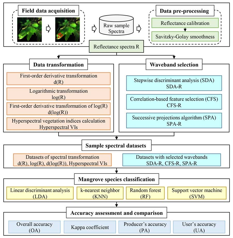
2. Materials and Methods

2.1. Study Area Description

Field hyperspectral measurements of this study were conducted at the Qi’ao Island Mangrove Nature Reserve, which has an area of 700 ha and is located on Qi’ao Island (22°23′40″–22°27′38″N, 113°36′40″–113°39′15″E), Zhuhai City, Guangdong Province, China [35,36] (Figure 2). Qi’ao Island is situated in Lingding Bay of the Pearl River Estuary, which has a typical tropical-subtropical transitional coastal-inland wetland ecosystem. Qi’ao Island belongs to the southern subtropical maritime monsoon climate zone, with sufficient sunshine and abundant rainfall [37,38]. The tidal pattern of Qi’ao Island is an irregular semidiurnal tide [8], which is characterized by the tidal height inequality of two adjacent high or low tides, the tide duration inequality between flood and ebb tides, and that the average tidal range varies with the flood and dry season, spring and neap tides [39]. The Mangrove Nature Reserve is the largest mangrove forest in the Pearl River Delta, it is the largest area of artificially planted mangrove forests in China and it has a rich variety of mangrove plants [8,36].
As shown in Figure 2, the field sampling route was along the boardwalks, in which the artificially planted mangrove forests were the dominant plant types. According to an existing research [37] and previous field surveys, there are eight common mangrove species in this study site, including Kandelia candel (K. candel), Acrostichum aureum (A. aureum), Acanthus ilicifolius (A. ilicifolius), Aegiceras corniculatum (A. corniculatum), Sonneratia apetala (S. apetala), Heritiera littoralis (H. littoralis), Cerbera manghas (C. manghas) and Therspesia populnea (T. populnea), as shown in Table 1. Among them, the K. candel stands were arbor or frutex, the A. aureum stands were herbage, the A. ilicifolius stands were frutex, and the other five stands were arbor. The C. manghas and T. populnea stands were semi-mangroves, and the other six stands were true mangroves.

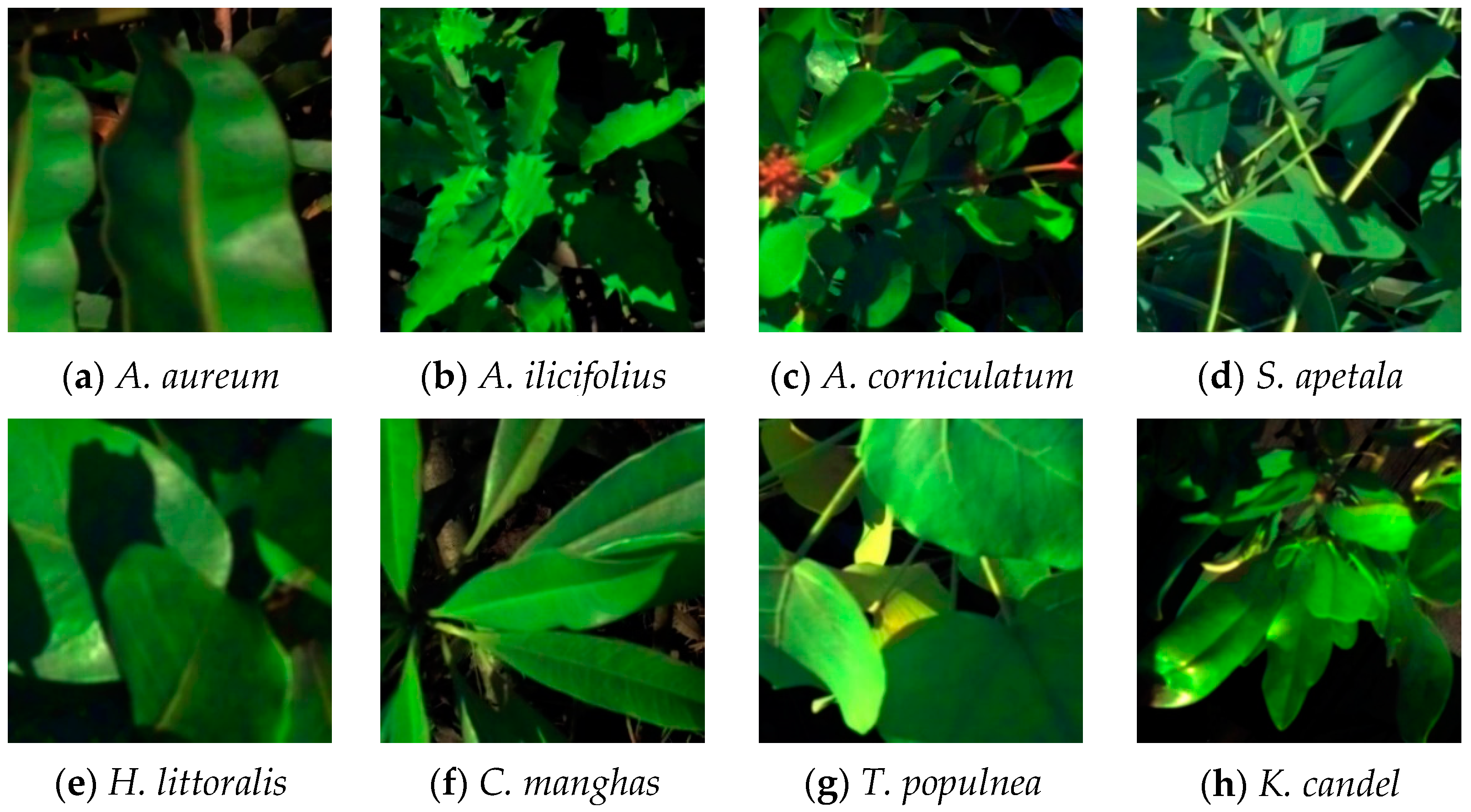
2.2. Data Acquisition and Sample Collection

2.2.1. Field Hyperspectral Measurement

For this study, the hyperspectral imaging system (Figure 3) was set up to acquire hyperspectral images of mangrove leaves. The main component of the experimental set-up was a commercial UHD 185 hyperspectral snapshot sensor (Figure 3a) manufactured by Cubert GmbH (http://cubert-gmbh.de/), Germany. The UHD 185 hyperspectral image consisted of a hyperspectral cube of 50 × 50 pixels and a panchromatic image with a resolution of 1000 × 1000 pixels. This sensor could capture 138 spectral bands within the spectral range of 450–998 nm with a 4-nm interval. According to previous studies [10,40], the spectral bands between 454 and 950 nm were used for analysis and classification. The UHD 185 sensor is currently applied onboard the UAV platform and can also be used for laboratory and ground-based spectrometry. This sensor was compact and lightweight with a total mass of about 470 g, which makes it highly portable and suitable for field applications, and it had a fast imaging speed of 5 cubes per second.
The main field hyperspectral measurements were performed on 3 January 2017. Due to the limitations on the accessibility of data collection site, data acquisition time, and illumination conditions on the day, several mangrove plants did not collect enough hyperspectral images. Therefore, part of the hyperspectral images of T. populnea and K. candel stands was collected as the supplementary data on 26 May 2018. Considering the influence of external illumination, the leaf spectra were collected on a cloud-free day at around solar noontime between 10:30 and 14:00. The UHD 185 hyperspectral imaging sensor could be hand-held and controlled by a notebook computer (Figure 3b). During the experiment, the spectral measurements were conducted above the mangrove canopy at approximately 20 cm height with the sensor facing and being at a near-vertical viewing direction to the canopy.

2.2.2. Data Pre-Processing

The field-collected spectra were radiometrically corrected with a standard white reference and dark measurements according to the pre-processing procedure used in a previous study [10]. Field-collected spectra are susceptible to variable illumination, contamination from the background environment and instrumental noise. To avoid noise associated with specific bands, the Savitzky–Golay algorithm [41,42] was introduced to smooth the raw hyperspectral data by eliminating glitch noise existing in the spectral curves. Based on least-squares fitting, this algorithm could remove high frequency noise and smooth the original data sequence by replacing the original values with fitted values [43], thereby preserving the original features of the spectrum. In this study, the Savitzky–Golay algorithm was implemented using the MATLAB R2014b software (MathWorks Inc., Natick, MA, USA).

2.2.3. Sample Spectra Preparation

Hyperspectral images of the eight mangrove plants of ground survey points were acquired with the UHD 185 hyperspectral imaging sensor. Representative images with true color composition of each mangrove species were shown in Figure 4. The sample collection strategy is as follows: (a) for each mangrove species, there are several ground survey points (Figure 1 and Table 1); (b) for each ground survey point, a preliminary manual screening was performed to select the hyperspectral images (Figure 4); and (c) for each hyperspectral image, there are five sample spectra were chosen. Considering that the illumination and background environment were the main factors related to the high spectral variability of the plant leaves [44], we selected spectral samples from the hyperspectral images of healthy and sun-lit mangrove leaves for each species with the Cube-Pilot software (Cubert GmbH, Ulm, Germany; http://cubert-gmbh.de/). For each type of mangrove species, 60 sample patches on the corresponding hyperspectral image were randomly selected (Table 1). A sample patch corresponded to 20 × 20 pixels in the selected cube which can be considered as a region of interest, and the spectral reflectance of the sample patch was calculated as the average value of pixels within the selected cube. A total of 480 sample spectra were selected. With these sample spectra, the 10-fold cross-validation was employed for the classification training and validation.

2.3. Hyperspectral Metrics Extraction

2.3.1. Data Transformation

Reflectance spectra from leaves in close-range imaging are often influenced by the illumination and background environment. Derivative spectra are commonly employed in hyperspectral investigations of vegetation [45], which can effectively reduce the influence of illumination variations, and eliminate the background signal and systematic errors. Previous studies have reported that the derivative analysis can further enhance the ability of the spectral data to identify tree species [46], and has been developed for mangrove species classification [47]. First-order derivative spectra can reflect the waveform changes caused by the absorption of the light by chlorophyll and other substances in plants, and reveal the peak characteristics of the spectrum [48]. Furthermore, because logarithmic transformation can enhance the spectral differences in the visible region and reduce the influence of multiplicative factors caused by changes in illumination conditions, we also performed the logarithmic transformation on spectral data. Following Pu and Gong [31], three transformations of R, including the first-order derivative of the reflectance spectra d(R), the logarithm of the reflectance spectra log(R) and its first-order derivative d[log(R)], were computed as
d ( R ) = ( r 3 r 1 Δ λ , r 4 r 2 Δ λ , , r n r n 2 Δ λ )
log ( R ) = [ log ( r 1 ) , log ( r 2 ) , , log ( r n ) ]
where r i denotes the i -th wavelength, n denotes the number of wavebands, and Δ λ denotes the double waveband intervals (nm).

2.3.2. Vegetation Index Calculation

Vegetation indices (VIs) are generally defined as mathematical transformations of the spectral reflectance of the original wavebands. One of the advantages of VIs is their ease of use. According to the definitions of VIs, they can enhance the differences between plant species and reveal the hidden vegetation information using various combinations of ratios, differences, and linear combinations [49,50]. Moreover, VIs can eliminate the influence of the multiplicative factor associated with illumination variations and background environments [31,51]. As shown in Table 2, we calculated 25 hyperspectral VIs, which were commonly used in previous studies [14,32,50] to identify and map plant species composition. These hyperspectral VIs were selected to represent spectral variations associated with pigments including chlorophylls, the leaf area index (LAI), biomass and red edge optical parameters, and so on.

2.4. Waveband Selection

Feature selection is an important pre-processing step for hyperspectral data, which can increase the efficiency of the classification model by removing irrelevant and redundant information [71]. Selecting the specific wavebands that are most important for developing more robust classification models is desirable [72,73]. In this study, three waveband selection methods, SDA, CFS and SPA, based on information entropy, correlation, and projection, respectively, were used to find out which wavebands can optimally differentiate mangrove species.

2.4.1. Stepwise Discriminant Analysis

The SDA is a multivariate statistical method, which has been used to discriminate variables. Based on the discriminant analysis, for each step, the variable with the strongest discriminative ability was introduced into the discriminant function, and the variable with the poorest discriminative ability was eliminated. In this manner, the SDA can be used to select a subset of wavebands that had the maximum discriminative ability [74]. In this study, the SDA was used to select the optimal wavebands according to the Wilks’ Lambda statistic [51], and implemented by the IBM SPSS Statistics 19 (IBM Inc., Armonk, NY, USA).

2.4.2. Correlation-Based Feature Selection

The CFS is a classic filter method for feature selection [75]. It has proven to be useful for selecting suitable features and facilitating computation. The idea of this algorithm is to calculate the “feature-class” and “feature-feature” correlation matrices from a training set. This algorithm assumes that these features are conditionally independent given the class. In this paper, the best first search algorithm [76] was applied for CFS to select the feature subset with the highest correlation between features and categories, and the lowest correlation between features and features. The CFS and best first search algorithms from the Weka 3.8 attribute selection package were used.

2.4.3. Successive Projections Algorithm

The SPA is a forward variable selection method, which has been used for waveband selection in previous studies [77]. The SPA randomly selects a starting waveband, calculates the maximum projection vector of an unselected waveband, and uses the corresponding waveband as the introduced waveband. After multiple iterations, the characteristic waveband is obtained by a cost function evaluation. This algorithm can effectively eliminate the influence of the collinearity that may exist among wavebands. In this study, the SPA selects the characteristic wavelengths that contain the least redundant information, which are determined by the minimum root mean square error of the prediction [78]. The SPA algorithm was implemented with MATLAB.

2.5. Mangrove Species Classification

We explored four mangrove species classification schemes using the LDA, KNN, RF, and SVM machine-learning classifiers based on the different datasets. These classification models were all executed in MATLAB.

2.5.1. Linear Discriminant Analysis

The LDA is a classic parametric algorithm in the field of data mining and machine learning, which has been widely used in previous classification researches to identify wetland plants, including mangroves [79,80,81]. The LDA determines the linear discriminant function based on the principle that the distance between classes is the largest and the distance within a class is the smallest, that is, to maximize the ratio of the dispersion between sample classes and minimize the dispersion within a sample class. The LDA makes two assumptions about the normal distribution of the data and the homoscedasticity for which two classes have equal covariance matrices. Finally, the category of unknown samples is determined by the established linear discriminant model.

2.5.2. K-Nearest Neighbor

The KNN is a non-parametric instance-based learning algorithm which has been extensively used for classification and regression [82]. The KNN is based on the assumption that ground objects close in distance are more likely to belong to the same category. The principle of KNN is that the instances within a dataset will generally exist in close proximity to other instances that have similar properties [83]. The distance between the feature vector to be classified and each feature vector in the feature space are calculated. The k nearest neighbor features are then selected. The categories of the testing sample are predicted by the majority vote of its neighbors using the Euclidean distance.

2.5.3. Random Forest

The RF is a non-parametric ensemble-based machine-learning method [84,85], which constructs a multitude of decision trees for learning and predicts the categories of the testing samples based on the average of the predicted values of each decision tree. The RF requires assumptions about independent variables and normality, and it does not need to check the variable interactions and nonlinear effects. The classification model of RF is mainly influenced by two parameters, including the number of decision trees (ntree) and the number of variables participating in the classification at the node (mtry). It distinguishes classes by individually building decision spaces for each explanatory variable at each node level, and the final classification ultimately depends on the decision spaces at higher nodes.

2.5.4. Support Vector Machine

The SVM is a well-known supervised kernel-based machine-learning method, and has proven to be one of the most widely used and efficient classifiers [86,87]. The SVM aims to find an optimal separating classification hyperplane which assumes that all groups are separable, to maximize the interval between the support planes of each type of data. It has powerful nonlinear and high-dimensional processing capabilities, which can avoid the “dimensionality disaster” caused by high-dimensional sample space and can be applied to small-sample learning. The LIBSVM package developed by Chang and Lin [88] has been widely used to implement the SVM classification model. Considering the nonlinear hyperplane, the radial basis function (RBF) kernel was chosen and two parameters, the cost of constraints (C) and sigma (σ), were determined by a grid search strategy.

2.6. Accuracy Assessment

For each of the classification results, we used a confusion matrix to provide the specific metrics, including the user’s accuracy (UA), the producer’s accuracy (PA), the overall accuracy (OA) and kappa coefficient (Kappa). The confusion matrix is an effective tool to evaluate the classification performance. It gives a full description of errors for each category, including the errors of inclusion and errors of exclusion made by the classifiers [89]. The PA denotes the probability of a certain category being correctly recognized. The UA denotes the probability that a sample belongs to a specific category, and the classifier can accurately sort it into this category. The main difference between PA and UA is the cardinality of the accuracy calculation [90]. For PA, the cardinality is the total number of categories by the reference samples. For UA, the cardinality is the total number of categories by the classified samples. PA is concerned with the quality of the method used to produce the classification result, while UA focuses on the credibility of each category in the classification result. The OA is the ratio (%) between the number of correctly classified samples and the number of testing samples [91]. The kappa coefficient is generally used to measure the agreement between the predicted and actual values [92,93].

3. Results

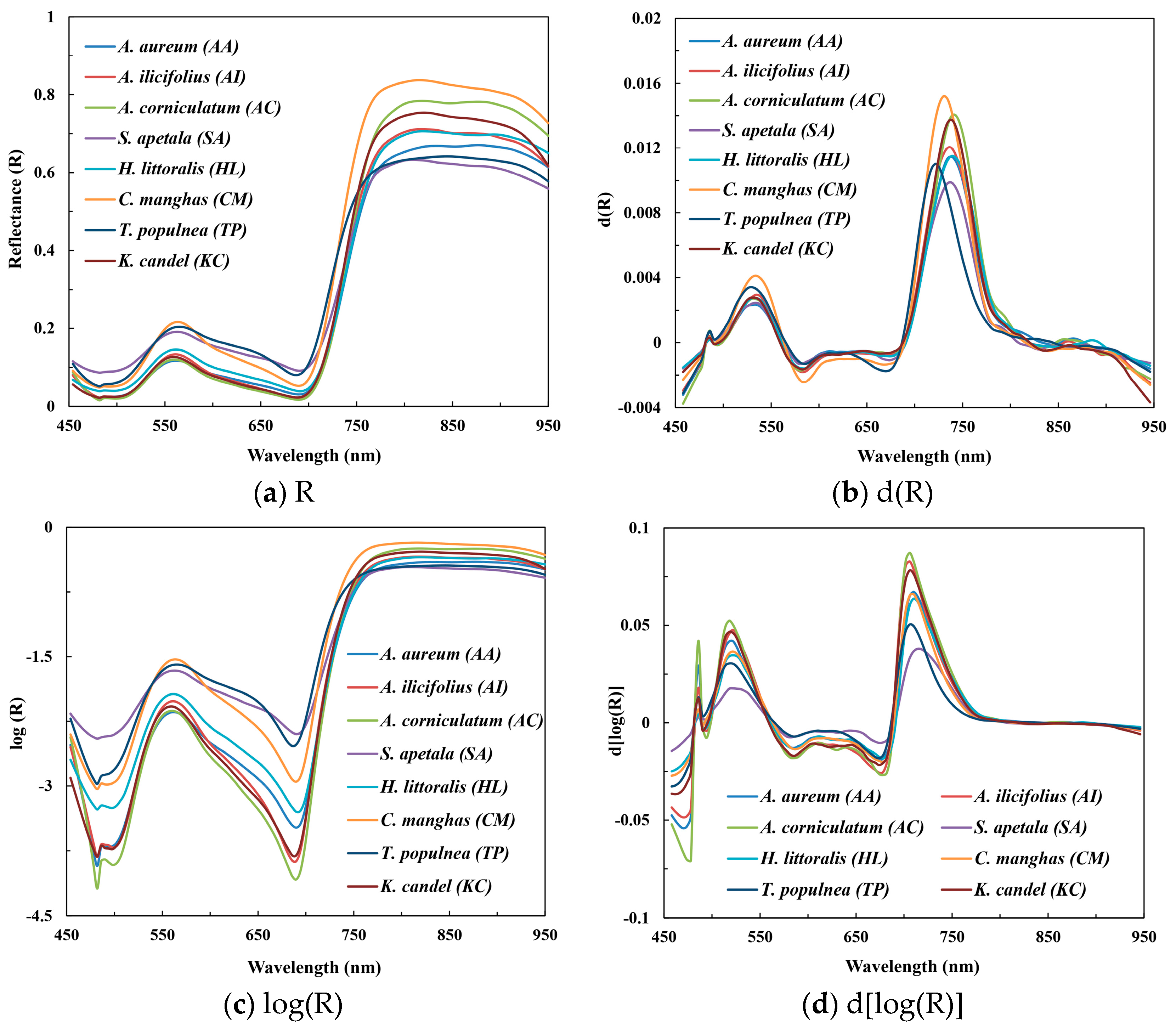
3.1. Spectral Properties of Mangrove Species

The average reflectance curves for the eight mangrove species (Figure 5a) showed typical patterns of vegetation. The trends in these spectral curves were generally similar, which increased continuously from 680 nm and reached a maximum peak around 780 nm, around the red edge region. The differences in the spectral response in the visible light region were indicative of leaf pigments. The mangrove leaves of C. manghas, T. populnea, and S. apetala stands had brighter green colors and consequently higher reflectance within the green reflectance spectral region. The near-infrared signal revealed the multiple scattering within the leaf structure. After the derivative and logarithmic transformations, the spectral variations within the species were reduced, while differences between species were enlarged. Figure 5b–d present the spectral curves of the first-order derivative of the reflectance spectra, the logarithm of the reflectance spectra and its first-order derivative of the leaves from the eight mangrove species, respectively.

3.2. Classification Results of the Transformed Datasets

Five hyperspectral datasets were used to identify mangrove species with the four machine-learning classifiers: (a) the reflectance spectra of all 125 wavebands R; (b) the first-order derivative of the reflectance spectra d(R); (c) the logarithm of the reflectance spectra log(R) and (d) its first-order derivative d[log(R)]; and (e) 25 hyperspectral VIs. Table 3 summarizes the classification accuracy assessment results. Based on hyperspectral VIs, the classification accuracies of the four classifiers were all more than 80%. Compared with the other three classifiers, SVM yielded a better overall classification accuracy of 93.54% (Kappa = 0.9253). Both the derivative and logarithmic transformations could improve the mangrove species classification accuracy. The discrimination capabilities of d(R) and log(R) spectral datasets were better than that from the reflectance spectra (Table 4). The d[log(R)]-classification using SVM gave the highest OA of 96.46% (Kappa = 0.9591). The producer’s and user’s accuracies of the eight mangrove species using SVM were all higher than 90%, especially for the A. aureum and S. apetala stands. This was mainly because the derivative and logarithmic transformations of reflectance spectra could reduce the multiplicative factors caused by changeable illumination conditions.

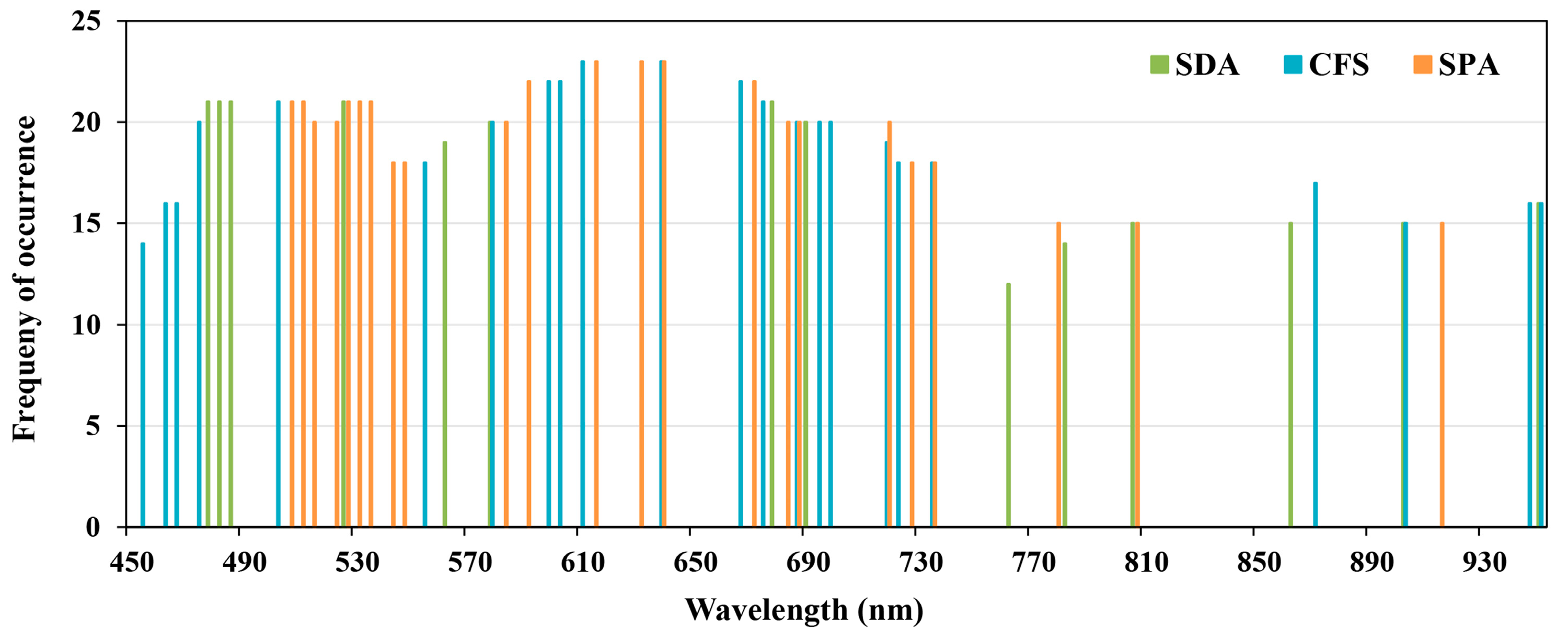
3.3. Optimal Waveband Selection

Considering the high dimensionality of the hyperspectral data and the spectral correlations among different mangrove species, it was necessary to select a few wavebands with lower correlation. For this study, three waveband selection methods, SDA, CFS and SPA, were used to determine the optimal wavebands, and their classification performances were compared. Table 5 shows the results of the effective wavebands selected by the three methods.
To examine the spectral separability of all the wavebands selected by the three methods, the one-way analysis of variance (ANOVA) and multiple significant comparative tests at the 99% confidence level (p < 0.01) were performed. As shown in Figure 6, most of the frequencies of occurrence of these selected wavebands were greater than 15 (half of C 8 2 ) [94,95], which showed their high discriminative capacity for mangrove species. The higher the frequency of occurrence, the more important the waveband, and the stronger the distinguishing ability of the mangrove species. The wavebands with higher frequencies of occurrence at 526 nm, 578 nm, 638 nm, 686 nm, 718 nm, 734 nm, 806 nm, 902 nm and 950 nm, which were selected by two or more waveband selection methods, showed their importance of classifying mangrove species.

3.4. Classification Results with the Selected Wavebands

The selected wavebands were then used as the input data for the LDA, KNN, RF and SVM classifications. Based on the reflectance spectra, the selected wavebands by using the three waveband selection methods (Table 5) and all 125 wavebands were used to identify mangrove species. Table 6 gives the classification results in terms of OA and kappa coefficient for the eight mangrove species identified by the four classifiers. The classification accuracies of these selected wavebands by using the SDA, CFS and SPA methods, were close to, or in some cases, higher than the accuracies when using all 125 wavebands. Among three waveband selection methods, the classification accuracy of the SPA was the highest. Hence, this report only presented the classification results of the wavebands selected by the SPA and the four classifiers (Table 7). Excepted for the LDA, the overall accuracies when using the other three classifiers all reach 80%, where the SVM was more than satisfactory in classifying mangrove species. The classification results indicated that the four classifiers could be easily used to identify the T. populnea stands, whose producer’s and user’s accuracies were more than 90%. For C. manghas, the classification accuracy of LDA was the lowest, while SVM could better separate C. manghas from other species, with a higher accuracy of 90%.

4. Discussion

4.1. Effect of the Optimal Waveband Selection Methods

The selection of effective wavebands can simplify the classification models and reduce the computational cost. By using a fewer number of effective wavebands is possible to achieve or exceed the classification accuracy of the entire waveband dataset [13]. The frequencies of occurrence of the selected wavebands demonstrated their high discriminative capacities for mangrove species (Figure 6), which were further verified by the classification results based on the wavebands selected by the three methods. The SDA method has been widely used for choosing effective wavebands in related research of mangroves [23], while the CFS and SPA methods have been mostly applied to machine-learning-based classifications [10,96]. In this study, the wavebands selected by the SPA showed better performance. There were few overlaps among the wavebands selected by the three methods (Table 5), while neighboring wavebands that had comparable discriminative capacities were selected. The wavebands at 526 nm, 578 nm, 638 nm, 686 nm, 718 nm, 734 nm, 806 nm, 902 nm and 950 nm were frequently selected. The selection results of this study differ from several studies with regards to the selected wavebands for classifying mangrove species [23,97]. This may be expected given the studied species and the specific sensor used in this study.

4.2. Impact of Spectral Datasets With Different Transformations

Spectral transformations and VIs can normally minimize the influence of brightness variations on ground-based spectral measurements. In this study, the classification performance of the selected hyperspectral VIs demonstrated that they were effective for the discrimination of vegetation species. This was consistent with the conclusion of a previous study [32]. Moreover, the derivative and log-transformed datasets manifested better classification results with the overall accuracies of all above 85%, when we employed the four machine-learning classifiers. When the classifications were performed based on the derivative spectra, the classification accuracy of LDA showed a slight improvement from 84.17% to 84.58% (Table 3). The LDA classifier generally requires the assumption of a normal distribution, while the derivative transformation will destroy this distribution [31]. Conversely, the logarithmic transformations can be generally used to normalize the distribution of a dataset. Based on the log-transformed dataset, the classification accuracy increment of LDA was 6.68%.

4.3. Performance of the Machine-Learning Classifiers

The classification performances of four machine-learning classifiers in identifying mangrove species were manifested, where most of the accuracies reached 80%. Compared to the other three non-parametric classifiers, the LDA gave the worst classification performance, especially when using fewer input parameters and the derivative spectra. This may be because the LDA is theoretically limited to parametric datasets and requires the assumption of normal distribution. As shown in Table 7, the lowest PA of 59.79% indicates that the LDA classifier has poor discrimination power for C. manghas class, and this class is easy to be mistakenly classified as another class. Conversely, the UA of 73.40% for C. manghas class shows that parts of the other classes were misclassified as this class. Previously, the non-parametric classifiers, such as RF and SVM, have proven to be effective for meeting the assumption of normal distribution when used for machine-learning classifications [34,98]. Overall, the SVM outperformed the KNN and RF classifiers, especially when using the selected wavebands and the derivative and log-transformed datasets. However, it should be noted that the classification performances of these machine-learning classifiers may generally depend on the number of features, number of samples, data types and the specific research purposes.

4.4. Applicability of Field Close-range Snapshot Hyperspectral Imaging

Hyperspectral imaging has been widely used to provide excellent detection capabilities for vegetation classification. The use of close-range snapshot hyperspectral imaging provides a new semi-automatic investigation method for hyperspectral measurements with proximal sensing in the field, which enables field surveys more convenient and rapid. The results of this study provided compelling evidence for the application of field close-range snapshot hyperspectral imaging in identifying mangrove species, which also provide a theoretical and practical guidance for monitoring mangrove forests. Compared to previous studies [22,23,24,25,26], which used non-imaging spectrometers, push-broom or staring imaging sensors, this hand-held close-range snapshot hyperspectral imaging, acquiring the spectral and image information at the time of one capture, bridges the gap between point and image data. It also can be considered as the transition from laboratory to field, and further close to realistic application. Furthermore, the snapshot hyperspectral imaging sensor can also be mounted on a UAV platform for use in precision agriculture, such as winter wheat above-ground biomass estimation [99], and vegetation classification [10,100]. The close-range hyperspectral imaging has potential to support the identifying of mangroves at the individual species level, but for field operational applications, there are still several limitations that need to be considered. Many captures need spend much time on preparations (e.g., multiple calibrations with white and dark references) and post-processing (e.g., the selection of samples), and the imaging effects are susceptible to the weather and illumination conditions.

5. Conclusions

In this study, we assessed the feasibility and usefulness of close-range snapshot hyperspectral imaging for mangrove species identification with field hyperspectral measurements. We classified mangrove species using different spectrum-transformed datasets, waveband selection methods, and machine-learning classifiers, and compared the classification results. Our main conclusions include: (1) The SVM proved to be more reliable for identifying mangrove species, when compared with the other three machine-learning classifiers. (2) The classification accuracies of the selected wavebands obtained by the three waveband selection methods, SDA, CFS and SPA, were competitive or comparable to the classification accuracies obtained when using all the wavebands. (3) The derivative and logarithmic transformations and hyperspectral VIs further improve the classification accuracies of mangrove species, especially those susceptible to background contamination and irregular illumination. The results of this study displayed the potential of close-range hyperspectral imaging as a tool in monitoring mangrove forests at the individual species level. The hyperspectral spectra of mangrove canopies acquired by using the snapshot hyperspectral imaging sensor under field conditions can be used to effectively identify mangrove species. The findings of this study can potentially provide further guidance for the application of space-borne and airborne hyperspectral sensors for mangrove forest management and conservation.

Author Contributions

J.C., K.L. and L.L. conceived and designed the experiments; J.C. performed the experiments and analyzed the results; J.C., K.L. and Y.Z. conducted the field investigations; J.C., K.L., L.L., J.L., and Z.H. wrote and revised the manuscript.

Funding

This research was jointly funded by the Science and Technology Planning Project of Guangdong Province (Grant No. 2017A020217003), the Natural Science Foundation of Guangdong (Grant No. 2016A030313261), the National Natural Science Key Foundation of China (Grant No. 41531178), the National Marine Public Welfare Research Project of China (Grant No. 201505012), the National Natural Science Foundation of China (Grant No. 61771496 and 41501368).

Acknowledgments

We would like to thank two doctoral students and three graduate students, including Cuilin Pan, Dashan Wang, Xiang Li, Min Tan and Liheng Peng, from the School of Geography and Planning, Sun Yat-sen University, Guangzhou, China, for their help during the field investigations. We also acknowledge China Oceanic Information Network, National Marine Data and Information Service (NMDIS) for providing the tidal data.

Conflicts of Interest

The authors declare no conflict of interest.

References

  1. Kuenzer, C.; Bluemel, A.; Gebhardt, S.; Quoc, T.V.; Dech, S. Remote sensing of mangrove ecosystems: A review. Remote Sens. 2011, 3, 878–928. [Google Scholar] [CrossRef]
  2. Giri, C. Observation and monitoring of mangrove forests using remote sensing: Opportunities and challenges. Remote Sens. 2016, 8, 783. [Google Scholar] [CrossRef]
  3. Bahuguna, A.; Nayak, S.; Roy, D. Impact of the tsunami and earthquake of 26th December 2004 on the vital coastal ecosystems of the Andaman and Nicobar islands assessed using RESOURCESAT AWiFS data. Int. J. Appl. Earth Obs. Geoinf. 2008, 10, 229–237. [Google Scholar] [CrossRef]
  4. Duke, N.C.; Meynecke, J.-O.; Dittmann, S.; Ellison, A.M.; Anger, K.; Berger, U.; Cannicci, S.; Diele, K.; Ewel, K.C.; Field, C.D. A world without mangroves? Science 2007, 317, 41–42. [Google Scholar] [CrossRef] [PubMed]
  5. Food and Agriculture Organization (FAO). The World’s Mangroves 1980–2005; FAO: Rome, Italy, 2007. [Google Scholar]
  6. Zhang, H.; Wang, T.; Liu, M.; Jia, M.; Lin, H.; Chu, L.; Devlin, A.T. Potential of combining optical and dual polarimetric SAR data for improving mangrove species discrimination using Rotation Forest. Remote Sens. 2018, 10, 467. [Google Scholar] [CrossRef]
  7. Pham, T.D.; Bui, D.T.; Yoshino, K.; Le, N.N. Optimized rule-based logistic model tree algorithm for mapping mangrove species using ALOS PALSAR imagery and GIS in the tropical region. Environ. Earth Sci. 2018, 77, 159. [Google Scholar] [CrossRef]
  8. Zhu, Y.; Liu, K.; Liu, L.; Myint, S.; Wang, S.; Liu, H.; He, Z. Exploring the potential of WorldView-2 red-edge band-based vegetation indices for estimation of mangrove leaf area index with machine learning algorithms. Remote Sens. 2017, 9, 1060. [Google Scholar] [CrossRef]
  9. Jia, M.; Zhang, Y.; Wang, Z.; Song, K.; Ren, C. Mapping the distribution of mangrove species in the Core Zone of Mai Po Marshes Nature Reserve, Hong Kong, using hyperspectral data and high-resolution data. Int. J. Appl. Earth Obs. Geoinf. 2014, 33, 226–231. [Google Scholar] [CrossRef]
  10. Cao, J.; Leng, W.; Liu, K.; Liu, L.; He, Z.; Zhu, Y. Object-based mangrove species classification using unmanned aerial vehicle hyperspectral images and digital surface models. Remote Sens. 2018, 10, 89. [Google Scholar] [CrossRef]
  11. Ruwaimana, M.; Satyanarayana, B.; Otero, V.; Muslim, A.M.; Syafiq, M.; Ibrahim, S.; Raymaekers, D.; Koedam, N.; Dahdouh-Guebas, F. The advantages of using drones over space-borne imagery in the mapping of mangrove forests. PLoS ONE 2018, 13, e0200288. [Google Scholar] [CrossRef] [PubMed]
  12. Wannasiri, W.; Nagai, M.; Honda, K.; Santitamnont, P.; Miphokasap, P. Extraction of mangrove biophysical parameters using airborne LiDAR. Remote Sens. 2013, 5, 1787–1808. [Google Scholar] [CrossRef]
  13. Tong, Q.; Zhang, B.; Zheng, L. Hyperspectral Remote Sensing: Principles, Techniques and Applications; Higher Education Press: Beijing, China, 2006. [Google Scholar]
  14. Thenkabail, P.S.; Lyon, J.G.; Huete, A. Hyperspectral Remote Sensing of Vegetation; CRC Press: Boca Raton, FL, USA, 2016. [Google Scholar]
  15. Kumar, T.; Panigrahy, S.; Kumar, P.; Parihar, J.S. Classification of floristic composition of mangrove forests using hyperspectral data: Case study of Bhitarkanika National Park, India. J. Coast. Conserv. 2013, 17, 121–132. [Google Scholar] [CrossRef]
  16. Chakravortty, S.; Sinha, D. Analysis of multiple scattering of radiation amongst end members in a mixed pixel of hyperspectral data for identification of mangrove species in a mixed stand. J. Indian Soc. Remote Sens. 2015, 43, 559–569. [Google Scholar] [CrossRef]
  17. Zhang, C.; Xie, Z. Data fusion and classifier ensemble techniques for vegetation mapping in the coastal everglades. Geocarto Int. 2014, 29, 228–243. [Google Scholar] [CrossRef]
  18. Green, E.P.; Clark, C.D.; Mumby, P.J.; Edwards, A.J.; Ellis, A. Remote sensing techniques for mangrove mapping. Int. J. Remote Sens. 1998, 19, 935–956. [Google Scholar] [CrossRef] [Green Version]
  19. Jensen, R.; Mausel, P.; Dias, N.; Gonser, R.; Yang, C.; Everitt, J.; Fletcher, R. Spectral analysis of coastal vegetation and land cover using AISA+ hyperspectral data. Geocarto Int. 2007, 22, 17–28. [Google Scholar] [CrossRef] [Green Version]
  20. Prasad, K.A.; Gnanappazham, L. Multiple statistical approaches for the discrimination of mangrove species of using transformed field and laboratory hyperspectral data. Geocarto Int. 2016, 31, 891–912. [Google Scholar] [CrossRef]
  21. Li, S.; Tian, Q. Mangrove canopy species discrimination based on spectral features of Geoeye-1 imagery. Spectrosc. Spectr. Anal. 2013, 33, 136–141. (In Chinese) [Google Scholar] [CrossRef]
  22. Vaiphasa, C.; Ongsomwang, S.; Vaiphasa, T.; Skidmore, A.K. Tropical mangrove species discrimination using hyperspectral data: A laboratory study. Estuar. Coast. Shelf Sci. 2005, 65, 371–379. [Google Scholar] [CrossRef]
  23. Zhang, C.; Kovacs, J.M.; Liu, Y.; Flores-Verdugo, F.; Flores-de-Santiago, F. Separating mangrove species and conditions using laboratory hyperspectral data: A case study of a degraded mangrove forest of the Mexican Pacific. Remote Sens. 2014, 6, 11673–11688. [Google Scholar] [CrossRef]
  24. Yu, X.; Zhang, F.; Liu, Q.; Li, D.; Zhao, D. Analysis of typical mangrove spectral reflectance characteristics. Spectrosc. Spectr. Anal. 2013, 33, 454–458. (In Chinese) [Google Scholar] [CrossRef]
  25. Yu, X.; Zhao, D.; Zhang, F.; Xiao, Z. Research on mangrove hyperspectrum analysis technology. J. Binzhou Univ. 2006, 22, 53–56. (In Chinese) [Google Scholar]
  26. Weng, Q.; Lu, C. Research on mangrove canopy apparent spectral reflectance characteristics. J. Fujian For. Sci. Technol. 2006, 33, 14–19. (In Chinese) [Google Scholar]
  27. Tian, M. Monitoring Winter Wheat Growth Conditions in the Northwest Region of China by Using Hyperspectral Remote Sensing. Ph.D. Dissertation, Northwest A&F University, Shanxi, China, 2017. (In Chinese). [Google Scholar]
  28. Shang, K.; Zhang, X.; Sun, Y.; Zhang, L.; Wang, S.; Zhuang, Z. Sophisticated vegetation classification based on feature band set using hyperspectral image. Spectrosc. Spectr. Anal. 2015, 35, 1669–1676. [Google Scholar] [CrossRef]
  29. Xiao, B.; Mao, W.; Liang, X.; Zhang, L.; Han, L. Study on varieties identification of Kentucky bluegrass using hyperspectral imaging and discriminant analysis. Spectrosc. Spectr. Anal. 2012, 32, 1620–1623. (In Chinese) [Google Scholar] [CrossRef]
  30. Gao, J.; Nuyttens, D.; Lootens, P.; He, Y.; Pieters, J.G. Recognising weeds in a maize crop using a random forest machine-learning algorithm and near-infrared snapshot mosaic hyperspectral imagery. Biosyst. Eng. 2018, 170, 39–50. [Google Scholar] [CrossRef]
  31. Pu, R.; Gong, P. Hyperspectral Remote Sensing and Its Applications; Higher Education Press: Beijing, China, 2000. [Google Scholar]
  32. Pu, R.; Gong, P. Hyperspectral remote sensing of vegetation bioparameters. In Advances in Environmental Remote Sensing: Sensors, Algorithms, and Applications; CRC Press: Boca Raton, FL, USA, 2011; pp. 101–142. [Google Scholar]
  33. Giri, S.; Mukhopadhyay, A.; Hazra, S.; Mukherjee, S.; Roy, D.; Ghosh, S.; Ghosh, T.; Mitra, D. A study on abundance and distribution of mangrove species in Indian Sundarban using remote sensing technique. J. Coast. Conserv. 2014, 18, 359–367. [Google Scholar] [CrossRef]
  34. Barrett, B.; Nitze, I.; Green, S.; Cawkwell, F. Assessment of multi-temporal, multi-sensor radar and ancillary spatial data for grasslands monitoring in Ireland using machine learning approaches. Remote Sens. Environ. 2014, 152, 109–124. [Google Scholar] [CrossRef] [Green Version]
  35. Liao, B.; Wei, G.; Zhang, J.; Tang, G.; Lei, Z.; Yang, X. Studies on dynamic development of mangrove communities on Qi’ao Island, Zhuhai. J. South China Agric. Univ. 2008, 29, 59–64. (In Chinese) [Google Scholar]
  36. Tang, H.; Liu, K.; Zhu, Y.; Wang, S.; Liu, L.; Song, S. Mangrove community classification based on WorldView-2 image and SVM method. Acta Sci. Nat. Univ. Sunyatseni 2015, 54, 102–111. (In Chinese) [Google Scholar]
  37. Zhou, F.; Kuang, D.; Jian, Y.; Huang, Q.; Ding, L. Primary study on the composition of mangrove community in Qi’ao Island, Zhuhai. Ecol. Sci. 2003, 22, 237–241. (In Chinese) [Google Scholar]
  38. Liu, K.; Liu, L.; Liu, H.; Li, X.; Wang, S. Exploring the effects of biophysical parameters on the spatial pattern of rare cold damage to mangrove forests. Remote Sens. Environ. 2014, 150, 20–33. [Google Scholar] [CrossRef]
  39. Ye, X.; Li, J.; Wang, A. Sedimentary environment and its response to anthropogenic impacts in the coastal wetland of the Qi’ao Island, Zhujiang River Estuary. Haiyang Xuebao 2018, 40, 79–89. [Google Scholar] [CrossRef]
  40. Aasen, H.; Burkart, A.; Bolten, A.; Bareth, G. Generating 3D hyperspectral information with lightweight UAV snapshot cameras for vegetation monitoring: From camera calibration to quality assurance. ISPRS-J. Photogramm. Remote Sens. 2015, 108, 245–259. [Google Scholar] [CrossRef]
  41. Savitzky, A.; Golay, M.J.E. Smoothing and differentiation of data by simplified least squares procedures. Anal. Chem. 1964, 36, 1627–1639. [Google Scholar] [CrossRef]
  42. Vaiphasa, C. Consideration of smoothing techniques for hyperspectral remote sensing. ISPRS-J. Photogramm. Remote Sens. 2006, 60, 91–99. [Google Scholar] [CrossRef]
  43. Zhao, A.; Tang, X.; Zhang, Z.; Liu, J. Optimizing Savitzky-Golay parameters and its smoothing pretreatment for FTIR gas spectra. Spectrosc. Spectr. Anal. 2016, 36, 1340–1344. (In Chinese) [Google Scholar] [CrossRef]
  44. Lopatin, J.; Fassnacht, F.E.; Kattenborn, T.; Schmidtlein, S. Mapping plant species in mixed grassland communities using close range imaging spectroscopy. Remote Sens. Environ. 2017, 201, 12–23. [Google Scholar] [CrossRef]
  45. Zhang, J.; Rivard, B.; Sánchez-Azofeifa, A.; Castro-Esau, K. Intra- and inter-class spectral variability of tropical tree species at La Selva, Costa Rica: Implications for species identification using HYDICE imagery. Remote Sens. Environ. 2006, 105, 129–141. [Google Scholar] [CrossRef]
  46. Qian, Y.; Yu, J.; Jia, Z.; Yang, F.; Palidan, T. Extraction and analysis of hyperspectral data from typical desert grassland in Xinjiang. Acta Pratacult. Sin. 2013, 22, 157–166. (In Chinese) [Google Scholar]
  47. Prasad, K.A.; Gnanappazham, L. Species discrimination of mangroves using derivative spectral analysis. ISPRS Ann. Photogramm. Remote Sens. Spat. Inf. Sci. 2014, 2, 45. [Google Scholar] [CrossRef]
  48. Becker, B.L.; Lusch, D.P.; Qi, J. Identifying optimal spectral bands from in situ measurements of Great Lakes coastal wetlands using second-derivative analysis. Remote Sens. Environ. 2005, 97, 238–248. [Google Scholar] [CrossRef]
  49. Pearson, R.L.; Miller, L.D. Remote mapping of standing crop biomass for estimation of the productivity of the shortgrass prairie. In Proceedings of the Eighth International Symposium on Remote Sensing of Environment, Ann Arbor, MI, USA, 2–6 October 1972; p. 1355. [Google Scholar]
  50. Sun, Y.; Gong, H. Quantitative Research on Wetland Plants Based on Hyperspectral Remote Sensing: A Case Study in Honghe Nature Reserve; China Environmental Science Press: Beijing, China, 2015. (In Chinese) [Google Scholar]
  51. Jain, N.; Ray, S.S.; Singh, J.P.; Panigrahy, S. Use of hyperspectral data to assess the effects of different nitrogen applications on a potato crop. Precis. Agric. 2007, 8, 225–239. [Google Scholar] [CrossRef]
  52. Zarco-Tejada, P.J.; Berjón, A.; López-Lozano, R.; Miller, J.R.; Martín, P.; Cachorro, V.; González, M.R.; De Frutos, A. Assessing vineyard condition with hyperspectral indices: Leaf and canopy reflectance simulation in a row-structured discontinuous canopy. Remote Sens. Environ. 2005, 99, 271–287. [Google Scholar] [CrossRef]
  53. Rouse, J.W.; Haas, R.H.; Schell, J.A.; Deering, D.W. Monitoring Vegetation Systems in the Great Plains with ERTS; Paper-A20; National Aeronautics and Space Administration (NASA): Washington, DC, USA, 1974; pp. 309–317.
  54. Roujean, J.L.; Breon, F.M. Estimating PAR absorbed by vegetation from bidirectional reflectance measurements. Remote Sens. Environ. 1995, 51, 375–384. [Google Scholar] [CrossRef]
  55. Haboudane, D.; Miller, J.R.; Pattey, E.; Zarco-Tejada, P.J.; Strachan, I.B. Hyperspectral vegetation indices and novel algorithms for predicting green LAI of crop canopies: Modeling and validation in the context of precision agriculture. Remote Sens. Environ. 2004, 90, 337–352. [Google Scholar] [CrossRef]
  56. Ar, H. A soil-adjusted vegetation index (SAVI). Remote Sens. Environ. 1988, 25, 295–309. [Google Scholar] [CrossRef]
  57. Baret, F.; Guyot, G. Potentials and limits of vegetation indices for LAI and APAR assessment. Remote Sens. Environ. 1991, 35, 161–173. [Google Scholar] [CrossRef]
  58. Qi, J.; Chehbouni, A.; Huete, A.R.; Kerr, Y.H.; Sorooshian, S. A modified soil adjusted vegetation index. Remote Sens. Environ. 1994, 48, 119–126. [Google Scholar] [CrossRef]
  59. Haboudane, D.; Miller, J.R.; Tremblay, N.; Zarco-Tejada, P.J.; Dextraze, L. Integrated narrow-band vegetation indices for prediction of crop chlorophyll content for application to precision agriculture. Remote Sens. Environ. 2002, 81, 416–426. [Google Scholar] [CrossRef]
  60. Rondeaux, G.; Steven, M.; Baret, F. Optimization of soil-adjusted vegetation indices. Remote Sens. Environ. 1996, 55, 95–107. [Google Scholar] [CrossRef]
  61. Daughtry, C.S.T.; Walthall, C.L.; Kim, M.S.; Colstoun, E.B.D.; McMurtrey, J.E.I. Estimating corn leaf chlorophyll concentration from leaf and canopy reflectance. Remote Sens. Environ. 2000, 74, 229–239. [Google Scholar] [CrossRef]
  62. Hernández-Clemente, R.; Navarro-Cerrillo, R.M.; Suárez, L.; Morales, F.; Zarco-Tejada, P.J. Assessing structural effects on PRI for stress detection in conifer forests. Remote Sens. Environ. 2011, 115, 2360–2375. [Google Scholar] [CrossRef]
  63. Broge, N.H.; Leblanc, E. Comparing prediction power and stability of broadband and hyperspectral vegetation indices for estimation of green leaf area index and canopy chlorophyll density. Remote Sens. Environ. 2000, 76, 156–172. [Google Scholar] [CrossRef]
  64. Jordan, C.F. Derivation of leaf-area index from quality of light on the forest floor. Ecology 1969, 50, 663–666. [Google Scholar] [CrossRef]
  65. Chen, J.M. Evaluation of vegetation indices and a modified simple ratio for boreal applications. Can. J. Remote Sens. 1996, 22, 229–242. [Google Scholar] [CrossRef]
  66. Zarcotejada, P.J.; Miller, J.R.; Noland, T.L.; Mohammed, G.H.; Sampson, P.H. Scaling-up and model inversion methods with narrowband optical indices for chlorophyll content estimation in closed forest canopies with hyperspectral data. IEEE Trans. Geosci. Remote Sens. 2001, 39, 1491–1507. [Google Scholar] [CrossRef] [Green Version]
  67. Vogelmann, J.E.; Rock, B.N.; Moss, D.M. Red edge spectral measurements from sugar maple leaves. Int. J. Remote Sens. 1993, 14, 1563–1575. [Google Scholar] [CrossRef]
  68. Gitelson, A.A.; Merzlyak, M.N.; Lichtenthaler, H.K. Detection of red edge position and chlorophyll content by reflectance measurements near 700 nm. J. Plant Physiol. 1996, 148, 501–508. [Google Scholar] [CrossRef]
  69. Zhang, C.; Chen, K.; Liu, Y.; Kovacs, J.M.; Flores-Verdugo, F.; Santiago, F.J.F.D. Spectral response to varying levels of leaf pigments collected from a degraded mangrove forest. J. Appl. Remote Sens. 2012, 6, 339–355. [Google Scholar] [CrossRef]
  70. Maire, G.L.; François, C.; Dufrêne, E. Towards universal broad leaf chlorophyll indices using prospect simulated database and hyperspectral reflectance measurements. Remote Sens. Environ. 2004, 89, 1–28. [Google Scholar] [CrossRef]
  71. Koedsin, W.; Vaiphasa, C. Discrimination of tropical mangroves at the species level with EO-1 Hyperion data. Remote Sens. 2013, 5, 3562–3582. [Google Scholar] [CrossRef]
  72. Vaiphasa, C.; Skidmore, A.K.; de Boer, W.F.; Vaiphasa, T. A hyperspectral band selector for plant species discrimination. ISPRS-J. Photogramm. Remote Sens. 2007, 62, 225–235. [Google Scholar] [CrossRef]
  73. Fung, T.; Yan Ma, H.F.; Siu, W.L. Band selection using hyperspectral data of subtropical tree species. Geocarto Int. 2003, 18, 3–11. [Google Scholar] [CrossRef]
  74. Thenkabail, P.S.; Enclona, E.A.; Ashton, M.S.; Meer, B.V.D. Accuracy assessments of hyperspectral waveband performance for vegetation analysis applications. Remote Sens. Environ. 2004, 91, 354–376. [Google Scholar] [CrossRef]
  75. Hall, M.A. Feature selection for discrete and numeric class machine learning. In Proceedings of the Seventeenth International Conference on Machine Learning, Stanford, CA, USA, 29 June–2 July 2000; pp. 359–366. [Google Scholar]
  76. Wollmer, M.; Schuller, B.; Eyben, F.; Rigoll, G. Combining long short-term memory and dynamic Bayesian networks for incremental emotion-sensitive artificial listening. IEEE J. Sel. Top. Signal Process. 2010, 4, 867–881. [Google Scholar] [CrossRef]
  77. Araújo, M.C.U.; Saldanha, T.C.B.; Galvão, R.K.H.; Yoneyama, T.; Chame, H.C.; Visani, V. The successive projections algorithm for variable selection in spectroscopic multicomponent analysis. Chemom. Intell. Lab. Syst. 2001, 57, 65–73. [Google Scholar] [CrossRef]
  78. Ma, H.; Ji, H.; Lee, W.S. Identification of the citrus greening disease using spectral and textural features based on hyperspectral imaging. Spectrosc. Spectr. Anal. 2016, 36, 2344–2350. [Google Scholar] [CrossRef]
  79. Clark, M.L.; Roberts, D.A.; Clark, D.B. Hyperspectral discrimination of tropical rain forest tree species at leaf to crown scales. Remote Sens. Environ. 2005, 96, 375–398. [Google Scholar] [CrossRef]
  80. Feret, J.B.; Asner, G.P. Tree species discrimination in tropical forests using airborne imaging spectroscopy. IEEE Trans. Geosci. Remote Sens. 2013, 51, 73–84. [Google Scholar] [CrossRef]
  81. Prospere, K.; McLaren, K.; Wilson, B. Plant species discrimination in a tropical wetland using in situ hyperspectral data. Remote Sens. 2014, 6, 8494–8523. [Google Scholar] [CrossRef]
  82. Cover, T.; Hart, P. Nearest neighbor pattern classification. IEEE Trans. Inf. Theory 1967, 13, 21–27. [Google Scholar] [CrossRef] [Green Version]
  83. Kotsiantis, S.B. Supervised machine learning: A review of classification techniques. In Proceedings of the 2007 Conference on Emerging Artificial Intelligence Applications in Computer Engineering: Real Word Ai Systems with Applications in Ehealth, Hci, Information Retrieval and Pervasive Technologies; IOS Press: Amsterdam, The Netherlands, 2007; pp. 3–24. ISBN 978-1-58603-780-2. [Google Scholar]
  84. Liaw, A.; Wiener, M. Classification and regression by randomforest. R News 2002, 2, 18–22. [Google Scholar]
  85. Naidoo, L.; Cho, M.A.; Mathieu, R.; Asner, G. Classification of savanna tree species, in the Greater Kruger National Park region, by integrating hyperspectral and LiDAR data in a Random Forest data mining environment. ISPRS-J. Photogramm. Remote Sens. 2012, 69, 167–179. [Google Scholar] [CrossRef]
  86. Féret, J.-B.; Asner, G.P. Semi-supervised methods to identify individual crowns of lowland tropical canopy species using imaging spectroscopy and LiDAR. Remote Sens. 2012, 4, 2457–2476. [Google Scholar] [CrossRef]
  87. Tan, Y.; Xia, W.; Xu, B.; Bai, L. Multi-feature classification approach for high spatial resolution hyperspectral images. J. Indian Soc. Remote Sens. 2017, 46, 9–17. [Google Scholar] [CrossRef]
  88. Chang, C.C.; Lin, C.J. Libsvm: A library for support vector machines. ACM Trans. Intell. Syst. Technol. 2011, 2, 27. [Google Scholar] [CrossRef]
  89. Stehman, S.V. Selecting and interpreting measures of thematic classification accuracy. Remote Sens. Environ. 1997, 62, 77–89. [Google Scholar] [CrossRef]
  90. Zhao, Y.; Chen, D.; Yang, L.; Li, X.; Tang, W. The Principle and Method of Analysis of Remote Sensing Application; Science Press: Beijing, China, 2003. [Google Scholar]
  91. Abdel-Rahman, E.M.; Mutanga, O.; Adam, E.; Ismail, R. Detecting sirex noctilio grey-attacked and lightning-struck pine trees using airborne hyperspectral data, random forest and support vector machines classifiers. ISPRS-J. Photogramm. Remote Sens. 2014, 88, 48–59. [Google Scholar] [CrossRef]
  92. Cohen, J. A coefficient of agreement for nominal scales. Educ. Psychol. Meas. 1960, 20, 37–46. [Google Scholar] [CrossRef]
  93. Cohen, J. Weighted kappa: Nominal scale agreement provision for scaled disagreement or partial credit. Psychol. Bull. 1968, 70, 213. [Google Scholar] [CrossRef] [PubMed]
  94. Lin, C.; Gong, Z.; Zhao, W.; Fan, L. Identifying typical plant ecological types based on spectral characteristic variables: A case study in Wild Duck Lake wetland, Beijing. Acta Ecol. Sin. 2013, 33, 1172–1185. [Google Scholar] [CrossRef]
  95. Huang, J.; Sun, Y. Sifting of hyperspectral vegetation indices applying to classification of 5 kinds of plants in Honghe wetlands. Wetl. Sci. 2016, 14, 888–894. (In Chinese) [Google Scholar]
  96. Zhu, H.; Chu, B.; Zhang, C.; Liu, F.; Jiang, L.; He, Y. Hyperspectral imaging for presymptomatic detection of tobacco disease with successive projections algorithm and machine-learning classifiers. Sci. Rep. 2017, 7, 4125. [Google Scholar] [CrossRef] [PubMed]
  97. Wang, L.E.; Sousa, W.P. Distinguishing mangrove species with laboratory measurements of hyperspectral leaf reflectance. Int. J. Remote Sens. 2009, 30, 1267–1281. [Google Scholar] [CrossRef]
  98. Pham, L.T.H.; Brabyn, L. Monitoring mangrove biomass change in Vietnam using spot images and an object-based approach combined with machine learning algorithms. ISPRS-J. Photogramm. Remote Sens. 2017, 128, 86–97. [Google Scholar] [CrossRef]
  99. Yue, J.; Yang, G.; Li, C.; Li, Z.; Wang, Y.; Feng, H.; Xu, B. Estimation of winter wheat above-ground biomass using unmanned aerial vehicle-based snapshot hyperspectral sensor and crop height improved models. Remote Sens. 2017, 9, 708. [Google Scholar] [CrossRef]
  100. Ishida, T.; Kurihara, J.; Viray, F.A.; Namuco, S.B.; Paringit, E.C.; Perez, G.J.; Takahashi, Y.; Marciano, J.J., Jr. A novel approach for vegetation classification using UAV-based hyperspectral imaging. Comput. Electron. Agric. 2018, 144, 80–85. [Google Scholar] [CrossRef]
Figure 1. Flowchart of mangrove species identification using field close-range snapshot hyperspectral imaging and machine-learning classifiers.
Remotesensing 10 02047 g001
Figure 2. Location of Qi’ao Island, showing the WorldView-2 image (false color composite composed of R, band 7; G, band 5; B, band 3). The map of field survey site was an UAV image (true color composition) acquired on 11 September 2015. The right panel shows a distribution map of 33 ground survey points, where the symbols in the legend indicate the sample locations along the boardwalks.
Remotesensing 10 02047 g002
Figure 3. Field hyperspectral measurements above the mangrove canopies and the set-up used to acquire the hyperspectral images. (a) The UHD 185 hyperspectral imaging sensor, and (b) a notebook computer.
Remotesensing 10 02047 g003
Figure 4. UHD 185 hyperspectral images of the eight mangrove species at the study site.
Remotesensing 10 02047 g004
Figure 5. The average reflectance curves, the spectral curves of derivative and logarithmic transformations of the eight mangrove species. (a) R: the average reflectance curves, (b) d(R): the average first-order derivative spectral curves, (c) log(R): the average log-transformed spectral curves, and (d) d[log(R)]: the average first-order derivative of the log-transformed spectral curves.
Remotesensing 10 02047 g005
Figure 6. Frequencies of occurrence of the selected wavebands using the SDA, CFS and SPA methods.
Remotesensing 10 02047 g006
Table 1. List of mangrove species used in this study.
Mangrove Species NameSpecies CodeFunctional GroupGround Survey PointsSamples
Acrostichum aureum (A. aureum)AAHerbage460
Acanthus ilicifolius (A. ilicifolius)AIFrutex460
Aegiceras corniculatum (A. corniculatum)ACArbor460
Sonneratia apetala (S. apetala)SAArbor460
Heritiera littoralis (H. littoralis)HLArbor460
Cerbera manghas (C. manghas)CMArbor460
Therspesia populnea (T. populnea)TPArbor660
Kandelia candel (K. candel)KCArbor/Frutex360
Table 2. Hyperspectral vegetation indices derived from the UHD 185 hyperspectral wavebands selected in this study.
Vegetation IndicesDefinitionCommonly Related toReferences
Blue Green Pigment Index 2 (BGI 2) R 454 R 550 Chlorophylls, Carotenoids[52]
Normalized Difference Vegetation Index (NDVI) R 798 R 670 R 798 + R 670 LAI, biomass, vegetation cover[53]
Reformed Difference Vegetation Index (RDVI) R 798 R 670 R 798 + R 670 LAI[54,55]
Soil-Adjusted Vegetation Index(SAVI) ( R 798 R 670 ) × ( 1 + 0.5 ) R 798 + R 670 + 0.5 Biomass[56]
Adjusted Transformed Soil-Adjusted VI (ATSAVI) a ( R 798 aR 670 b ) aR 798 + R 670 ab + X ( 1 + a 2 )
where X = 0.08, a = 1.22, b = 0.03
LAI, biomass, soil variation[57]
Modified SAVI (MSAVI) R 798 + 0.5 ( R 798 + 0.5 ) 2 2 ( R 798 R 670 ) Biomass, soil variation[58]
Transformed Chlorophyll Absorption in Reflectance Index (TCARI) 3 [ ( R 702 R 670 ) 0.2 ( R 702 R 550 ) × ( R 702 R 670 ) ] Chlorophylls[59]
Optimized Soil-Adjusted Vegetation Index (OSAVI) ( 1 + 0.16 ) × R 798 R 670 R 798 + R 670 + 0.16 Biomass, soil variation[60]
TCARI/OSAVI TCARI OSAVI Chlorophylls[59]
Modified Chlorophyll Absorption in Reflectance Index (MCARI) [ ( R 702 R 670 ) 0.2 ( R 702 R 550 ) ] × ( R 702 R 670 ) Chlorophylls[61]
Modified Chlorophyll Absorption Ratio Index 1 (MCARI1) 1.2 [ 2.5 ( R 798 R 670 ) 1.3 ( R 798 R 550 ) ] LAI[55]
Modified Chlorophyll Absorption Ratio Index 2 (MCARI 2) 1.5 [ 2.5 ( R 798 R 670 ) 1.3 ( R 798 R 550 ) ] ( 2 R 798 + 1 ) 2 ( 6 R 798 5 R 670 ) 0.5 Chlorophylls[55]
Photochemical Reflectance Index (PRI) R 514 R 530 R 514 + R 530 Water content[40,62]
Triangular Vegetation Index (TVI) 0.5 [ 120 ( R 750 R 550 ) 200 ( R 670 R 550 ) ] LAI[63]
Modified Triangular VI 1 (MTVI 1) 1.2 [ 1.2 ( R 798 R 550 ) 2.5 ( R 670 R 550 ) ] LAI[55]
Modified Triangular VI 2 (MTVI 2) 1.5 [ 1.2 ( R 798 R 550 ) 2.5 ( R 670 R 550 ) ] ( 2 R 798 + 1 ) 2 ( 6 R 798 5 R 670 ) 0.5 LAI[55]
Simple Ratio (SR) R 798 R 670 Chlorophylls[51,64]
Modified Simple Ratio (MSR) ( R 798 R 670 1 ) / R 798 R 670 + 1 LAI[55,65]
Zarco Tejada and Miller (ZTM) R 750 R 710 Red edge[66]
Vogelmann Red Edge Index 1 (VOG1) R 742 R 722 Red edge[67]
Vogelmann Red Edge Index 2 (VOG2) R 734 R 750 R 718 + R 726 Red edge[66]
Vogelmann Red Edge Index 3 (VOG3) R 734 R 750 R 718 + R 722 Red edge[66]
Red Edge NDVI (RENDVI) R 754 R 702 R 754 + R 702 Red edge[68]
Vogelmann’s Index (VOI) DR 718 DR 706 Red edge[67,69]
Modified Simple Ratio of Derivatives (DMSR) DR 722 DR 502 DR 722 + DR 502 Chlorophylls[70]
Note: R denotes the reflectance spectra, DRi denotes the first-order derivative of the reflectance spectra.
Table 3. Classification results in terms of OA (overall accuracy), kappa coefficient, and standard deviation (in bracket) for the eight mangrove species using different spectral datasets and classifiers of the 10-fold cross-validation data.
Spectral DatasetsPerformance
Metrics
Classifiers
LDAKNNRFSVM
Reflectance spectra
R
OA(%)84.17
(5.22)
87.50
(5.29)
87.92
(4.03)
93.54
(2.68)
Kappa0.8179
(0.0595)
0.8562
(0.0607)
0.8609
(0.0460)
0.9256
(0.0308)
Hyperspectral VIsOA(%)85.00
(4.79)
84.58
(5.12)
85.83
(5.62)
93.54
(2.07)
Kappa0.8270
(0.0544)
0.8223
(0.0585)
0.8366
(0.0652)
0.9253
(0.0244)
First-order derivative spectra d(R)OA(%)84.58
(6.45)
90.63
(3.84)
92.71
(3.57)
95.83
(2.20)
Kappa0.8218
(0.0736)
0.8917
(0.0437)
0.9156
(0.0410)
0.9518
(0.0252)
Log-transformed spectra log(R)OA(%)89.79
(3.73)
88.54
(4.20)
86.04
(4.40)
93.75
(4.39)
Kappa0.8823
(0.0431)
0.8681
(0.0478)
0.8396
(0.0505)
0.9281
(0.0505)
First-order derivative of log(R) d[log(R)]OA(%)85.83
(7.07)
95.00
(3.43)
92.29
(3.55)
96.46
(2.42)
Kappa0.8367
(0.0812)
0.9421
(0.0398)
0.9112
(0.0408)
0.9591
(0.0280)
Table 4. Summary of classification accuracies and standard deviation (in bracket) of the d[log(R)] spectral dataset using different classifiers of the 10-fold cross-validation data.
Mangrove SpeciesClassifiers
LDAKNNRFSVM
PA(%)UA(%)PA(%)UA(%)PA(%)UA(%)PA(/%)UA(%)
A. aureum (AA)81.86
(20.30)
92.46
(10.59)
93.65
(8.40)
94.31
(10.89)
93.15
(9.40)
90.06
(11.67)
98.75
(3.95)
100.00
(0.00)
A. ilicifolius (AI)90.25
(14.26)
88.65
(15.81)
94.67
(11.67)
93.89
(11.25)
93.83
(10.12)
89.08
(8.20)
96.33
(7.77)
95.76
(10.61)
A. corniculatum (AC)85.33
(17.26)
86.11
(16.47)
93.00
(16.36)
88.99
(8.19)
84.71
(14.72)
85.50
(13.83)
95.89
(9.45)
93.00
(12.01)
S. apetala (SA)98.33
(5.27)
92.00
(9.76)
98.57
(4.52)
94.72
(9.11)
97.50
(5.27)
97.50
(5.27)
98.57
(4.52)
98.89
(3.51)
H. littoralis (HL)82.88
(15.53)
93.99
(7.85)
89.40
(16.61)
97.32
(5.66)
87.64
(9.06)
92.05
(10.88)
90.24
(17.83)
97.14
(6.02)
C. manghas (CM)69.30
(21.82)
67.90
(21.61)
91.65
(9.08)
98.00
(6.32)
89.23
(12.82)
95.00
(8.05)
93.24
(8.83)
96.07
(8.66)
T. populnea (TP)97.32
(5.66)
90.74
(11.40)
100.00
(0.00)
98.75
(3.95)
98.75
(3.95)
92.08
(13.95)
100.00
(0.00)
97.50
(5.27)
K. candel (KC)83.17
(19.44)
87.64
(14.97)
96.00
(8.43)
96.67
(10.54)
94.75
(8.70)
98.33
(5.27)
98.00
(6.32)
96.33
(7.77)
OA(%)85.83 (7.07)95.00 (3.43)92.29 (3.55)96.46 (2.42)
Kappa0.8367 (0.0812)0.9421 (0.0398)0.9112 (0.0408)0.9591 (0.0280)
Table 5. The selected wavebands, based on the reflectance spectra, using the SDA, CFS and SPA methods.
MethodsSelected Wavebands (nm)
SDA14 bands: 478–482, 486, 526, 562, 578, 678, 690, 762, 782, 806, 862, 902, 950
CFS23 bands: 454, 462–466, 474, 502, 554, 578, 598–602, 610, 638, 666, 674, 686, 694–698, 718–722, 734, 870, 902, 946–950
SPA23 bands: 506–514, 522–534, 542–546, 582, 590, 614, 630, 638, 670, 682–686, 718, 726, 734, 778, 806, 914
Table 6. Classification results in terms of OA, kappa coefficient, and standard deviation (in bracket) for the eight mangrove species obtained using different selected wavebands and classifiers of the 10-fold cross-validation data.
Selected WavebandsPerformance
Metrics
Classifiers
LDAKNNRFSVM
125 wavebandsOA(%)84.17
(5.22)
87.50
(5.29)
87.92
(4.03)
93.54
(2.68)
Kappa0.8179
(0.0595)
0.8562
(0.0607)
0.8609
(0.0460)
0.9256
(0.0308)
14 wavebands
(SDA)
OA(%)74.79
(7.04)
86.46
(5.31)
86.04
(5.38)
91.46
(4.10)
Kappa0.7104
(0.0812)
0.8442
(0.0609)
0.8394
(0.0617)
0.9017
(0.0471)
23 wavebands
(CFS)
OA(%)81.67
(7.47)
87.92
(4.59)
87.71
(4.33)
92.29
(2.79)
Kappa0.7896
(0.0852)
0.8608
(0.0527)
0.8586
(0.0498)
0.9112
(0.0321)
23 wavebands
(SPA)
OA(%)83.75
(3.51)
86.88
(4.29)
84.58
(4.93)
93.13
(1.98)
Kappa0.8133
(0.0400)
0.8490
(0.0489)
0.8226
(0.0565)
0.9208
(0.0227)
Table 7. Summary of classification accuracies and standard deviation (in bracket) using different classifiers of the 10-fold cross-validation data with the 23 wavebands selected by the SPA.
Mangrove SpeciesClassifiers
LDAKNNRFSVM
PA(%)UA(%)PA(%)UA(%)PA(%)UA(%)PA(%)UA(%)
A. aureum (AA)84.88
(12.70)
77.84
(15.44)
93.99
(7.85)
76.31
(16.02)
86.37
(11.50)
77.55
(14.20)
93.89
(8.11)
84.43
(13.84)
A. ilicifolius (AI)87.75
(14.55)
92.14
(15.95)
84.57
(15.14)
82.17
(15.95)
75.81
(16.34)
77.89
(11.32)
90.40
(14.09)
89.87
(9.47)
A. corniculatum (AC)96.67
(10.54)
69.55
(15.29)
72.08
(16.43)
90.50
(12.96)
71.33
(20.25)
80.75
(18.93)
80.71
(15.02)
96.57
(7.35)
S. apetala (SA)76.62
(21.44)
98.33
(5.27)
98.33
(5.27)
93.57
(8.33)
97.08
(6.23)
96.90
(6.55)
100.00
(0.00)
98.57
(4.52)
H. littoralis (HL)83.68
(17.68)
80.25
(14.68)
90.07
(14.31)
87.57
(13.23)
84.95
(17.91)
79.92
(13.45)
94.57
(12.95)
88.50
(10.64)
C. manghas (CM)59.79
(31.60)
73.40
(28.72)
80.90
(22.09)
90.07
(14.31)
83.57
(22.23)
87.64
(12.49)
91.67
(21.15)
96.14
(9.23)
T. populnea (TP)98.57
(4.52)
98.57
(4.52)
96.67
(7.03)
90.05
(11.09)
95.42
(7.47)
93.17
(9.90)
100.00
(0.00)
98.33
(5.27)
K. candel (KC)83.99
(15.28)
90.07
(14.31)
75.92
(13.46)
94.25
(9.72)
82.32
(16.24)
92.98
(9.53)
89.17
(14.72)
97.50
(7.91)
OA(%)83.75 (3.51)86.88 (4.29)84.58 (4.93)93.13 (1.98)
Kappa0.8133 (0.0400)0.8490 (0.0489)0.8226 (0.0565)0.9208 (0.0227)

