Abstract
Extreme-learning machines (ELM) have attracted significant attention in hyperspectral image classification due to their extremely fast and simple training structure. However, their shallow architecture may not be capable of further improving classification accuracy. Recently, deep-learning-based algorithms have focused on deep feature extraction. In this paper, a deep neural network-based kernel extreme-learning machine (KELM) is proposed. Furthermore, an excellent spatial guided filter with first-principal component (GFFPC) is also proposed for spatial feature enhancement. Consequently, a new classification framework derived from the deep KELM network and GFFPC is presented to generate deep spectral and spatial features. Experimental results demonstrate that the proposed framework outperforms some state-of-the-art algorithms with very low cost, which can be used for real-time processes.
1. Introduction
Hyperspectral imagery in remote sensing with hundreds of narrow spectral bands is used in many applications, such as global environment monitoring, land cover change detection, natural disaster assessment and medical diagnosis [1,2,3,4] etc. Classification is a significant information acquisition technique for hyperspectral imagery, which focuses on distinguishing physical objects and classifying each pixel into a unique label. With the development of machine learning, most machine learning algorithms based on statistical learning theory are employed in the information processing field. There are many traditional classification algorithms, such as k-nearest neighbors (KNN) [5], Bayesian models [6], random forests [7], etc. One of the most important and famous classifiers for hyperspectral image classification is the kernel-based support vector machine (KSVM), which can also be considered to be a neural network [8,9]. It provides superior classification performance by learning an optimal decision hyperplane to best separate different classes in a high-dimensional feature space through non-linear mapping. Some popular kernels include polynomial function and Gaussian radial basis function (RBF).
Recently, deep neural networks (DNNs) have been highlighted in the literature, which can learn high-level features hierarchically [10,11,12,13]. DNNs have demonstrated their potential in classification; in particular, they have motivated successful applications of deep models in hyperspectral image classification, which outperform other traditional classification methods. The typical deep-learning architectures include stacked autoencoders (SAEs) [14], deep belief networks (DBNs) [15] and convolutional neural networks (CNNs) [16,17]. Chen et al. first employed SAE depth model to extract features of hyperspectral imagery and classify these features via logical regression [18]. Then, Chen et al. used DBN as a classifier to distinguish each pixel [19]. In addition, Li and Du proposed a hyperspectral classification model which combines an optimized DBN with a texture feature enhancement model, achieving superior classification accuracy [20]. In particular, due to its local receptive fields, CNNs play a dominant role for processing the visual-based issues. Hu et al. employed a CNN to classify hyperspectral images directly in spectral domain [21]. However, without enough training samples, the traditional CNN faces an over-fitting problem. Li et al. proposed a fully CNN for feature enhancement and obtained outstanding hyperspectral accuracy [22]. Nevertheless, due to the high computation cost and space complexity, the aforementioned algorithms are very time-consuming. Real-time application is the predominant trend in future hyperspectral processing, and most of the aforementioned algorithms may not meet the requirements in fast data processing and analysis.
Extreme-learning machine (ELM) as a very fast and effective machine learning algorithm with a single hidden-layer feed-forward neural network was proposed by Huang in [23]. The parameters between its input and hidden layers are simply random variables. The only parameters to be trained are output weights, which can be easily estimated by a smallest norm least-squares solution. Compared with the traditional gradient-based back propagation (BP) learning, ELM is computationally much more efficient than the SVM and BP neural networks. Therefore, plentiful works about ELM have already done in hyperspectral classification [24,25,26,27] and achieved acceptable contributions. However, with the randomly generated weights and bias of ELM, it leads to different results even with the same hidden nodes. The kernel-based ELM (KELM) [28] was proposed to overcome this problem, which employs a kernel function to replace the hidden layer of the ELM. In [29,30], KELM has been used for hyperspectral image classification and obtained appreciate results. However, the feature representation ability is limited of the shallow networks. Therefore, multilayer solutions are imperative. Inspired by the multilayer perception (MLP) theory, Huang extended ELM to a multilayer ELM (ML-ELM) through using ELM-based autoencoder (ELM-AE) for feature representation and extraction [31]. From the perspective of deep learning, ELM-AE is stacked by deep layers can further extract deep robust and abstract features. In [32], the ML-ELM and KELM were combined for handling the EEG classification, where the former acted as a feature extractor and the latter as a classifier. The architecture of the method is complex and too much hyperparameters need to be determined. Additionally, several studies [33,34,35,36] have focused on integrating spatial and spectral information in hyperspectral imagery to assist classification. Multi-features are extracted and employed for classification. For instance, Kang et al. used a guided filter to process the pixel-wise classification map in each class by using the first-principal component (PC) or the first three PCs to capture major spatial features [37].
In this paper, we firstly investigate the ML-ELM for its suitability and effectiveness for hyperspectral classification. Then, to acquire desirable performance, we promote a deep layer-based kernel ELM (DKELM) algorithm to extract the deep and robust features of hyperspectral imagery. In addition, spatial information through different filters is added to further enhance the classification accuracy. The main contributions of this paper are summarized below:
- ML-ELM is investigated and applied firstly in hyperspectral classification.
- A classification framework is proposed for hyperspectral classification which combines DKELM and a novel guided filtering first-principal component (GFFPC) spatial filter.
- The DKELM model remains simple, because randomly generated parameters are not necessary but only kernel parameters need to be tuned in each layer. Furthermore, compared to the ML-ELM, the numbers of nodes for each hidden layer are not required to be set due to the kernel tricks.
- The proposed framework can achieve superior performance with very fast training speed, which is beneficial for real-time application.
This paper is organized as follows. Section 2 briefly introduces the ELM, KELM and ML-ELM (for convenience, we use MELM to replace ML-ELM in the following sections). Section 3 proposes our new framework to address the hyperspectral classification problem. Section 4 depicts the datasets and parameters tuning. Experimental results are presented and discussed in Section 5. The conclusions are drawn in Section 6.
2. Related Works
2.1. ELM and KELM
The ELM is a single hidden-layer feed-forward neural network (SLFN) as depicted in Figure 1. Please note that the hidden layer is non-linear because of the use of a non-linear activation function. However, the output layer is linear without an activation function. It contains three layers: input layer, hidden layer, and output layer.
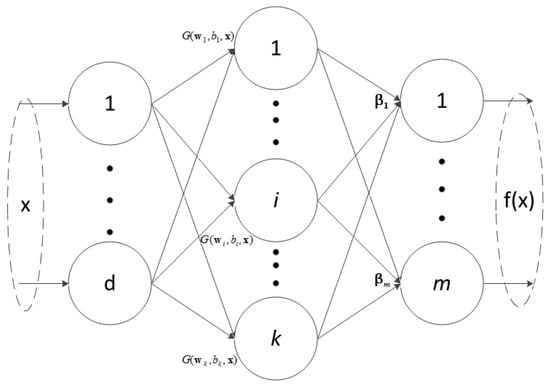
Figure 1.
The structure of ELM.
Let represent a training sample and be the output of the neural network. The SLFN with k hidden nodes can be represented by the following equation:
where denotes the hidden-layer activation function, is the input weight matrix connecting the input layer to the hidden layer, b means the bias weight of the hidden layer, and is the weight between the hidden layer and output layer. For an ELM with n training samples, d input neurons (i.e., the number of bands), k hidden neurons, and m output neurons (i.e., m classes), Equation (1) becomes
where is the m-dimensional desired output vector for the i-th training sample , the d-dimensional represents the j-th weight vector from the input layer to the j-th hidden neuron, and is the bias of the j-th hidden neuron. Here, denotes the inner product of and . The sigmoid function g is used as the activation function, so the output of the j-th hidden neuron is
where denotes the exponent arithmetic, and is the steepness parameter.
In matrix form, model (2) can be rearranged as
where is the target output, . is referred to as hidden-layer output matrix of ELM with the size of , which can also be expressed as follows:
Then, can be estimated by a smallest norm least-squares solution:
where C is a regularization parameter. The ELM model can be represented as
ELM can be extended to kernel-based ELM (KELM) via using kernel trick. Let
in which
where and represent the i-th and j-th training sample, respectively. Then, replacing by , the representation of KELM can be written as
where represents the output of the KELM model, and .
Obviously, different from ELM, the most important characteristic of KELM is that the number of hidden nodes is not desired to be set and there are no random feature mappings. Furthermore, the computing time is reduced compared with ELM due to the kernel trick used.
2.2. Multilayer Extreme-Learning Machines (MELM)
Figure 2 depicts the detailed structure of ELM autoencoder(ELM-AE). ELM-AE represents features based on singular values. MELM is a multilayer neural network through stacking multiple ELM-AEs.
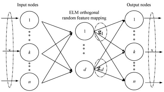
Figure 2.
The structure of ELM-AE: both the input and output are , and ELM-AE has the same solution as the original ELM. is the d-th hidden node for input .
Let , where is the i-th data representation for input , k=1 to n. Suppose is the i-th transformation matrix, where is the transformation vector used for representation learning with respect to . According to Equation (4), is replaced by and is replaced by respectively in MELM.
where is the output matrix of the i-th hidden layer with respect to , and can be solved by
Then
where is the last representation of . is used as hidden-layer output to calculate the output weight and can be computed as
3. The Proposed Framework for Hyperspectral Classification
In this section, we propose a new framework for hyperspectral classification which combines the hyperspectral spatial features with the Deep-layer-based KELM. The details of the proposed framework are discussed in this section. The main procedure of our proposed framework is briefly depicted in Figure 3. From Figure 3, we can see that the major three parts are as follows: data normalization, spatial feature enhancement and DKELM classification. The following sections introduce these three procedures in detail.
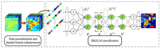
Figure 3.
The main procedure of our proposed framework. is the first layer’s transformation matrix of DKELM got from the KELM-AE of the input data. refers to the transformation matrix of - hidden layer of DKELM, which obtained by KELM-AE of the i-th hidden layer .
3.1. Data Normalization
Let be a hyperspectral data, where N denotes the number of samples and L is the number of bands. Data normalization is the pre-procedure to make each sample standardization. For each sample:
where is the normalized sample, , and and denote the mean and variance of the samples, respectively. After this process, the data has zero mean and unit variance.
3.2. Spatial Features Enhancement
In our proposed framework, we use the Gaussian filters to extract spatial information; furthermore, a spatial feature enhancement method combined with guided filter (GF) and principal component analysis (PCA) is presented to enhance spatial information. Here, we introduce the GFFPC in detail.
The GF was proposed by He in 2012 [38], which can be used as an edge-preserving filter such as bilateral filter and it performs better near edges with fast time. As a local linear model, GF assumes that output image o is a linear transformation of guidance image g in a window of size * centered at the pixel k, where = (2r + 1):
where is the i-th pixel of the output image o and is the i-th pixel of guidance image g, respectively. It is obvious that this model ensures , which means the output o will have an edge only if g has an edge. To calculate the coefficients and , a minimum energy function is applied as follows:
where is the i-th pixel of the input image, and is a regularization parameter penalizing large , which can affect the blurring for the GF. According to the energy function, it is expected that the output image o ought to be as close as possible to the input image f, while preserving the texture information of guidance image g through the linear model.
The solution to (16) can be addressed by linear regression as follows (Draper, 1981):
where and are the mean and variance of guidance image g within the local window , respectively. is the number of pixels in . In addition, is the mean value of f in the window.
The structure of GFFPC is shown in Figure 4. We can see that the original hyperspectral image is processed by PCA method firstly, then we get the reconstructed dataset consisting of a new set of independent bands named PCs. After that, the GF is performed on each band of the original dataset, where the first PC of the reconstructed dataset is used as the gray-scale guidance image with the most information of the hyperspectral image including spatial features. The filtering output is the novel hyperspectral data cube with more distinctive edges and texture features, that can help further hyperspectral classification.
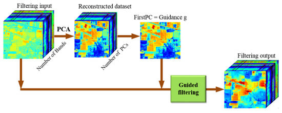
Figure 4.
The structure of GFFPC.
3.3. DKELM Classification
DKELM consists of several KELM-auto-encoders (AEs) in deep layer. Thus, we firstly present a brief description of the KELM-AE.
3.3.1. KELM-AE
Figure 5 demonstrates the structure of KELM-AE which is very similar to ELM-AE except the kernel representation. The kernel operation in Figure 5 can be represented as
is referred to as the testing samples, denotes the j-th training sample, and is the mapping function to the reproducing kernel Hilbert space(RKHS). From Figure 5, the input matrix is mapped into a kernel matrix through kernel function . In our proposed DKELM, we use the RBF kernel function with parameter .
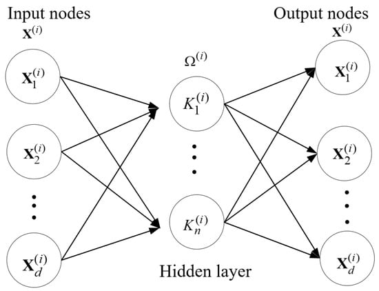
Figure 5.
The structure of KELM-AE.
Then is employed to represent the i-th transformation matrix in KELM-AE, which is similar to ELM-AE in (10)
and then is calculated via
The data can be represented through the final data transformation procedure using:
where g is still an activation function. The hidden-layer activation functions can be either linear or non-linear. In our proposed DKELM, we use non-linear activation functions. Because deep distinct and abundant features can be learned and captured through the data representation via non-linear activation functions used between each KELM-AE. The combination of dense and sparse representations has more powerful interpretation than only linear learning. Compared to ELM-AE, we can find that the number of hidden nodes is not necessary to be set in advance because of the kernel trick used in each hidden layer. The pseudocode of KELM-AE is depicted in Algorithm 1.
3.3.2. DKELM
DKELM can obtain the universal approximation due to two separate learning procedures contained as same as in H-ELM [31]. Each pair of and (in the i-th KELM-AE) can be computed via Equations (19) and (23), respectively. At last, the final data representation is calculated, and then is used as the training input to train a KELM classification model as:
where is obtained from , then the output weight can be calculated via
The procedure of DKELM is depicted in Algorithm 2, including the training and testing phases.
| Algorithm 1 The pseudocode of KELM-AE. |
| Input: Input matrix , regularization parameter , kernel parameter , activation function . Output: Transformation matrix , new data representation . Step1: Calculate the kernel matrix , where and are referred to as the k-th and j-th training sample, respectively. Step2: Calculate the output weight . Step3: Calculate the new data representation . Return: , . |
| Algorithm 2: The pseudocode of DKELM. |
Output: Transformation matrix for each hidden layer, the final representation of the training samples and final output weight of the output layer. Step1: for do: Calculate end. Step2: Step3: Calculate , where and are the final representation of the training samples and respectively. Step4: Calculate the final output weight . Return –, , .
Output: Output matrix of the testing samples . Step1: for do: Calculate the hidden representation end. Step2: Step3: Calculate the kernel matrix , where and are the final representation of the training samples and the final representation of the testing sample , respectively. Step4: Calculate the final output of the DKELM . |
MELM employs the pseudoinverse to calculate the transformation matrix in each layer. Compared to MELM, exact inverse is used to calculate via invertible kernel matrix in the KELM-AEs of DKELM. Therefore, a theoretically perfect reconstruction of is resulted, which will reduce the error accumulation of the AEs in a certain degree. Consequently, DKELM can learn a better data representation and make for better generalization.
4. Experiments
In this section, we design a series of experiments to evaluate our proposed hyperspectral framework combining spatial filters with DKELM. As the comparison algorithms, ELM, KELM, KSVM and CNN are used in our experiments. Besides, all these algorithms are combined with GFFPC spatial feature enhancement method for further comparison purpose. The evaluation criteria employed are overall accuracy (OA) and kappa coefficient. Three classic hyperspectral benchmark datasets and one self-photographed hyperspectral dataset, noted as Indian Pines, University of Pavia, Salinas and Glycine ussuriensis, are used. In this paper, except CNN, all experiments are performed using MATLAB R2017b on a computer with 3.2 GHz CPU and 8.0 GB RAM. CNN algorithm is performed on NVIDIA Tesla K80 GPU.
4.1. Hyperspectral Datasets
The Indian Pines dataset was gathered by Airborne Visible/Infrared Imaging Spectrometer (AVIRIS) sensor in North-western Indiana. It contains 220 spectral bands from 0.4–2.45 m region with spatial resolution of 20 m. This image has 145 × 145 pixels with 200 bands after removing 20 noisy and water absorption bands. The Indian Pines scene includes two-third agriculture, and one-third forest. The groundtruth of this image is introduced in Figure 6. Sixteen classes are contained and their numbers of labeled samples are tabulated in Table 1. In Indian Pines, 10% to 50% of labeled data of each class is selected randomly as training samples, and the remaining is testing samples.
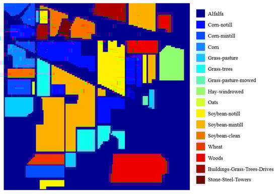
Figure 6.
The groundtruth of Indian Pines.

Table 1.
Labeled samples in Indian Pines dataset.
The second dataset we used is about the University of Pavia, an urban scene acquired by the Reflective Optics Spectrometer (ROSIS) sensor. The ROSIS sensor can generate 115 spectral bands over 0.43 to 0.86 m. This image scene has 610 × 340 pixels, and each pixel has 103 bands after noisy band removal. The geometric resolution is 1.3 m per pixel. The Nine groundtruth classes with the number of labeled samples are tabulated in Table 2. Figure 7 demonstrates the groundtruth of the Pavia University using as the referenced image. In Pavia University, 5% to 25% of labeled data of each class used as training samples to evaluate the proposed framework.
Table 2.
Labeled samples in University of Pavia.
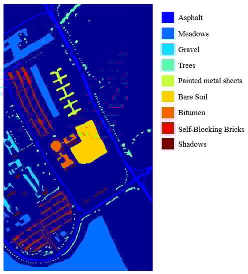
Figure 7.
The groundtruth of University of Pavia.
The third dataset is named Salinas which was also collected by the 224-band AVIRIS sensor over Salinas Valley, California. This image scene comprises 512 × 217 pixels. It has 204 bands after removing noisy and water absorption bands. The groundtruth depicted in Figure 8 contains 16 classes and the detailed samples are showed in Table 3. In Salinas dataset experiments, 5% to 25% of labeled samples of each class are chosen randomly for training our proposed classification framework.
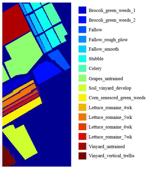
Figure 8.
The groundtruth of Salinas Dataset.
Table 3.
Labeled samples in Salinas Dataset.
The last dataset is named Glycine ussuriensis dataset which was collected over the Yellow River Delta National Nature Reserve, Qingdao, China. The image is acquired by the Nano-hyperspec imaging system equipped on unmanned aerial vehicle. This image scene comprises 355 × 266 pixels with 270 bands after removing noisy and water absorption bands. The Glycine ussuriensis dataset contains 4 classes shown in Figure 9 and Table 4. All four categories are plants, specifically, Glycine ussuriensis is a small-seeded species, which is grown in hills, roadsides, or shrubs at 100–800 m above sea level. Unlike the datasets mentioned before, the classes in Glycine ussuriensis have no strict geographical separation. For instance, the samples in tarragon are surrounded by other samples. In the experiments, 5% to 25% of labeled samples of each class are chosen randomly to testify our proposed classification framework.
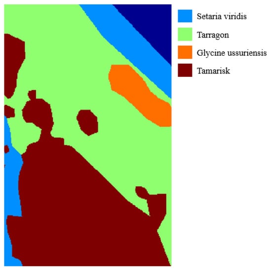
Figure 9.
The groundtruth of Glycine Ussuriensis Dataset.
Table 4.
Labeled samples in Glycine Ussuriensis Dataset.
4.2. Parameters Tuning and Setting
In our proposed framework, we need to tune several parameters. There are two user specified parameters are required for GFFPC, the size of local sliding window denoted and the regularization parameter denoted , respectively, in which the latter determining the degree of the blurring for the GF. In the simulations, is chosen from [3, 5, 7, 9, 11], and is selected in the range of [1e-1, 1e-2, 1e-3, 1e-4, 1e-5, 1e-6]. Figure 10a shows the classification accuracies of DKELM in the subspace, where the parameter is prefixed. It can be seen that better performance is achieved when equals 7 for all the datasets. Then Figure 10b indicates the impact on the classification results of different . The OA first increased, and then decreased as decreasing. Thus, we set to 1e-4 finally.
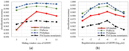
Figure 10.
The impact on the classification results of different parameters of GFFPC (a) local sliding window size , (b) regularization parameter .
Figure 11 shows the accuracies obtained with different numbers of kernel layers in DKELM. We can see that in the case of using three kernel layers, the classification performance of DKELM can achieve superior results, because, based on the characteristics of hyperspectral datasets, three kernel layers of the network can already extract sufficient refined and distinguished features for the classification task, and the over-fitting occurs when the network is too deep with limited training samples. Thus, in our proposed framework, we set the number of kernel layers to 3.
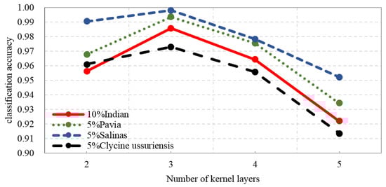
Figure 11.
The accuracies obtained with different numbers of kernel layers in DKELM.
Kernel function we used in this paper is RBF. The activation functions employed to connect different KELM-AEs are sigmoid and ReLU function. Sigmoid function can constrain the output of each layer to the range from 0 to 1, which has been represented in Equation (3). The ReLU function [39] can be expressed as follows:
where x is the input. The ReLU leads a sparse learning which can decrease the relationship among the parameters and eliminate the over-fitting problem. Therefore, the combination of sigmoid and ReLU functions can learn deep feature with different scales, which is beneficial to DKELM. Our proposed DKELM has three kernel layers, therefore three main parameters need to be tuned. are the parameters used in RBF kernel functions. To make full advantages of our framework, a gird search algorithm is employed in tuning . Figure 12 depicts the detailed tuning procedures of the three parameters in Indian Pines, University of Pavia, Salinas, and Glycine ussuriensis datasets, respectively. The vertical coordinate axis represents , and the two horizontal coordinate axes express . The color bars in Figure 12 mean the classification accuracy obtained via the different sets of values. The black circle with best classification accuracy depicts the values we finally chosen. Here, we list the final chosen values employed in the four datasets: {4e2, 3.6e3, 5.2e7} , {2.9e2, 1e5, 6e6}, {4e2, 5e4, 8e6} and {4e2, 3.6e3, 6e7}.
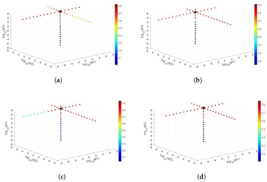
Figure 12.
Parameters tuning of DKELM in (a) Indian pines, (b) University of Pavia, (c) Salinas, and (d) Glycine ussuriensis Datasets.
5. Experimental Results and Discussions
In this section, the proposed GFFPC and the novel classification model will be assessed, and the related results will be summarized and discussed at length. All the algorithms are repeated 10 runs with different locations of the training samples for each dataset, and the mean results with the corresponding standard deviation are reported.
5.1. Discussion on the Proposed GFFPC
In the experiments, we first investigate the impact of different spatial filters to MELM and DKELM. Figure 13 illustrates the OA of different spatial filters based on MELM and DKELM algorithms. Origin denotes the performance obtained via the original MELM and DKELM. G_3 × 3 and G_5 × 5 mean using Gaussian filter with 3 × 3 and 5 × 5 size of windows respectively before employing MELM and DKELM. The GFFPC represents using GFFPC based on MELM and DKELM.
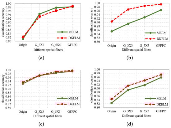
Figure 13.
The performance of different spatial filters combined with MELM and DKELM in (a) Indian pines, (b) University of Pavia, (c) Salinas, and (d) Glycine ussuriensis Datasets.
From Figure 13, We can see that the performance with spatial filters become better than without spatial filters. Furthermore, the GFFPC obtains superior performance to Gaussian filters. Consequently, in our subsequent experiments, the GFFPC filter is our recommended spatial filter for strongly enhancing spatial features.
5.2. Discussion on the Classification Results
Table 5 tabulates the performance achieved by different classification algorithms and the combinations with GFFPC spatial filter through using 10% of labeled samples as training samples in Indian Pines. Although the OA of DKELM is slightly worse than the performance of CNN, our proposed framework DKELM-GFFPC outperforms other classification algorithms. In addition, quite apart from that, our proposed GFFPC can enhance the classification performance by a wide range. For instance, the OA of ELM-GFFPC is increased by 16.23% and the OA of CNN-GFFPC has been improved from 83.19% to 95.57%. In particular, the performance of MELM and DKLEM are enhanced by 17.02% and 16.38%, respectively. For class 1, 9 and 16 of Indian Pines, the accuracies increase from 83.33%, 66.67% and 98.33% to 100%, 94.44% and 100% when DKELM-GFFPC is used instead of DKELM. This phenomenon indicates that our proposed framework can beneficial to the performance of several small-size classes.
Table 5.
Classification Accuracy(%) of the comparison and proposed algorithms in Indian Pines.
Table 6 also lists the classification performance of the comparison algorithms and the proposed algorithm in University of Pavia dataset through using 5% labeled samples as training samples. From the accuracies exhibited in Table 6, the OA of DKELM is improved by 13.95% via using GFFPC spatial filter. The performance of other algorithms is also enhanced in different degrees from 2.6% to 11.29%. It also can be seen that after combining with GFFPC, the classification performance is enhanced greatly. In particular, the DKELM-GFFPC achieves the best performance. Furthermore, the accuracies of small-size classes such as classes 5, 7 and 9 are improved through using GFFPC, implying that GFFPC can keep more distinctive features of small-size classes.
Table 6.
Classification Accuracy(%) of the comparison and proposed algorithms in University of Pavia.
Table 7 demonstrates the performance obtained via different classification algorithms in Salinas dataset through adopting 5% of labeled samples as training samples. Compared with other algorithms, the proposed DKELM-GFFPC is still a predominant one. In addition, the classification performance of ELM, KELM, KSVM, CNN, MELM and DKELM is increased by 5.86%, 7.81%, 6.21%, 6.43%, 6.61% and 6.22%, respectively. Furthermore, classes 11, 13 and 14 are small classes with a few training samples, the performances of which are enhanced greatly through using the GFFPC spatial filter.
Table 7.
Classification Accuracy(%) of the comparison and proposed algorithms in Salinas Dataset.
The classification accuracies achieved through the Glycine ussuriensis dataset are tabulated in Table 8. From Table 8, the DKELM-GFFPC obtains best performance than other classification frameworks. GFFPC still has the positive influence on enhancing the classification performance. For instance, the OAs of MELM and CNN are improved by 13.41% and 12.48% through adding GFFPC spatial filter. Moreover, the classification accuracy of the class Glycine ussuriensis with the least labeled samples is enhanced greatly through our proposed spatial filter and classification framework.
Table 8.
Classification Accuracy(%) of the comparison and proposed algorithms in Glycine ussuriensis Dataset.
From Table 5, Table 6, Table 7 and Table 8, we can see that CNN, MELM and DKELM can work better than other traditional classifiers. Therefore, to further testify our proposed framework, we compare DKELM-GFFPC with CNN-GFFPC and MELM-GFFPC when using different percentage of training samples in Figure 14. With the increasing training samples, the classification performance is increasing gradually. Obviously, DKELM-GFFPC outperforms other two classification frameworks regardless the number of training samples. One of the most significant advantages of the proposed classification framework is the very fast training procedure. Thus, the average training times of different algorithms are compared and demonstrated in Table 9. ELM-based methods are faster than KSVM and CNN. The training time of DKELM and KELM depend on the number of training data. Meanwhile, ELM and MELM rely on the number of hidden neurons. The more the hidden neurons, the more the training time since the higher model generalization is provided subject to the data complexity. CNN can achieve superior classification performance. Nevertheless, it spends more training time which is nearly 135 to 411 times than that of DKELM in different experimental datasets. Therefore, DKELM is the most appealing one with the best performance and the least training time.
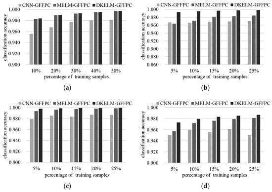
Figure 14.
The performance of CNN, MELM and DKELM combined with GFFPC through using different size of training sample in (a) Indian pines, (b) University of Pavia, (c) Salinas, and (d) Glycine ussuriensis Dataset.
Table 9.
Training time (In second) of different algorithms based on four datasets.
To illustrate the merits of our proposed classification framework and the spatial filter from the perspective of visualization, Figure 15, Figure 16, Figure 17 and Figure 18 demonstrate the classification maps. Clearly, compared with the groundtruth shown in Figure 6, Figure 7, Figure 8 and Figure 9, the classification maps obtained by our proposed framework are the smoothest and clearest. Besides, the classification maps achieved with GFFPC spatial filter are more distinct than without evidently. In particular, the border pixels and the boundaries of different classes in DKELM-GFFPC are more distinct. Compared with other classification methods, our proposed framework is better because of less salt-an-pepper noise contained in the classification maps.
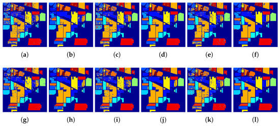
Figure 15.
Classification maps of the (a) ELM, (b) ELM + GFFPC, (c) KELM, (d) KELM + GFFPC, (e) KSVM, (f) KSVM + GFFPC, (g) CNN, (h) CNN + GFFPC, (i) MELM, (j) MELM + GFFPC, and the proposed (k) DKELM, and (l) DKELM + GFFPC for the Indian Pines.
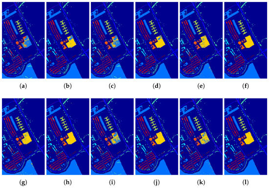
Figure 16.
Classification maps of the (a) ELM, (b) ELM + GFFPC, (c) KELM, (d) KELM + GFFPC, (e) KSVM, (f) KSVM + GFFPC, (g) CNN, (h) CNN + GFFPC, (i) MELM, (j) MELM + GFFPC, and the proposed (k) DKELM, and (l) DKELM + GFFPC for the University of Pavia.
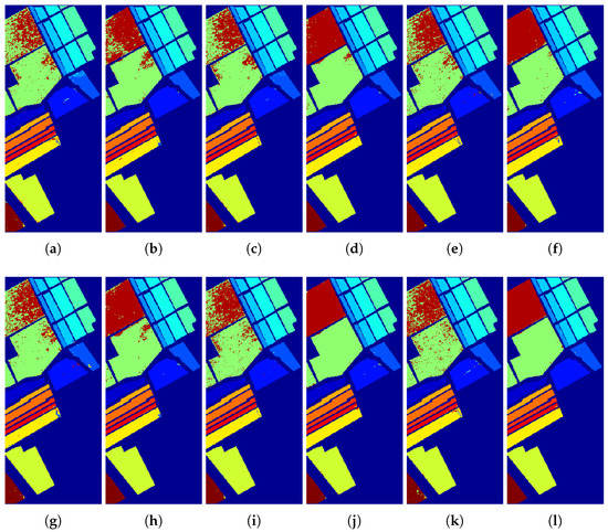
Figure 17.
Classification maps of the (a) ELM, (b) ELM + GFFPC, (c) KELM, (d) KELM + GFFPC, (e) KSVM, (f) KSVM + GFFPC, (g) CNN, (h) CNN + GFFPC, (i) MELM, (j) MELM + GFFPC, and the proposed (k) DKELM, and (l) DKELM + GFFPC for the Salinas dataset
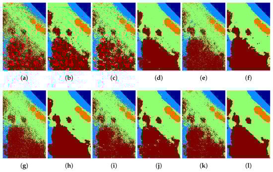
Figure 18.
Classification maps of the (a) ELM, (b) ELM + GFFPC, (c) KELM, (d) KELM + GFFPC, (e) KSVM, (f) KSVM + GFFPC, (g) CNN, (h) CNN + GFFPC, (i) MELM, (j) MELM + GFFPC, and the proposed (k) DKELM, and (l) DKELM + GFFPC for the Glycine ussuriensis dataset.
6. Conclusions
In this work, the MELM algorithm is investigated and firstly applied to hyperspectral classification. Then, a DKELM-GFFPC framework is proposed consisting of the GFFPC for enhancing spatial features and the DKELM, a kernel version of MELM. Experimental results demonstrate that it can outperform other traditional algorithms, especially, DKELM-GFFPC can improve the accuracy of those classes with small-size samples in a different degree for each dataset. Moreover, compared with Gaussian filter, the proposed GFFPC can play an important role in enhancing hyperspectral classification performance. Finally, our proposed classification framework takes much lowest computation cost to achieve the highest classification accuracy. Based on the above-mentioned advantages, we believe that the proposed hyperspectral classification framework based on the novel DKELM and GFFPC is more suitable to process hyperspectral data in practical applications with low cost of computing, furthermore, in real-time application.
Author Contributions
J.L. and Q.D. conceived and designed the study; B.X. performed the experiments; G.R. and R.S. shared part of the experiment data; J.L. and Y.L. analyzed the data; J.L. and B.X. wrote the paper. Y.L., Q.D. and R.S. reviewed and edited the manuscript. All authors read and approved the manuscript.
Acknowledgments
This work was partially supported by the Fundamental Research Funds for the Central Universities JB170109, General Financial Grant from the China Postdoctoral Science Foundation (no. 2017M623124) and Special Financial Grant from the China Postdoctoral Science Foundation (no. 2018T111019). It was also partially supported by the National Nature Science Foundation of China (no. 61571345, 91538101, 61501346 and 61502367) and the 111 project (B08038).
Conflicts of Interest
The authors declare that we have no financial and personal relationships with other people or organizations that can inappropriately influence our work and this paper was not published before, the founding sponsors had no role in the design of the study; in the collection, analyses, or interpretation of data; in the writing of the manuscript, and in the decision to publish the results.
References
- Shan, J.; Zhao, J.; Liu, L.; Zhang, Y.; Wang, X.; Wu, F. A novel way to rapidly monitor microplastics in soil by hyperspectral imaging technology and chemometrics. Environ. Pollut. 2018, 238, 121–129. [Google Scholar] [CrossRef]
- Liu, K.; Su, H.; Li, X. Estimating High-Resolution Urban Surface Temperature Using a Hyperspectral Thermal Mixing (HTM) Approach. IEEE J. Sel. Top. Appl. Earth Obs. Remote Sens. 2016, 9, 804–815. [Google Scholar] [CrossRef]
- Haboudane, D.; Tremblay, N.; Miller, J.R.; Vigneault, P. Remote Estimation of Crop Chlorophyll Content Using Spectral Indices Derived From Hyperspectral Data. IEEE Trans. Geosci. Remote Sens. 2008, 46, 423–437. [Google Scholar] [CrossRef]
- Pike, R.; Lu, G.; Wang, D.; Chen, Z.G.; Fei, B. A Minimum Spanning Forest-Based Method for Noninvasive Cancer Detection With Hyperspectral Imaging. IEEE Trans. Biomed. Eng. 2016, 63, 653–663. [Google Scholar] [CrossRef]
- Li, W.; Du, Q.; Zhang, F.; Hu, W. Collaborative-Representation-Based Nearest Neighbor Classifier for Hyperspectral Imagery. IEEE Geosci. Remote Sens. Lett. 2015, 12, 389–393. [Google Scholar] [CrossRef]
- Rankin, B.M.; Meola, J.; Eismann, M.T. Spectral Radiance Modeling and Bayesian Model Averaging for Longwave Infrared Hyperspectral Imagery and Subpixel Target Identification. IEEE Trans. Geosci. Remote Sens. 2017, 55, 6726–6735. [Google Scholar] [CrossRef]
- Zhang, Y.; Cao, G.; Li, X.; Wang, B. Cascaded Random Forest for Hyperspectral Image Classification. IEEE J. Sel. Top. Appl. Earth Obs. Remote Sens. 2018, 11, 1082–1094. [Google Scholar] [CrossRef]
- Melgani, F.; Bruzzone, L. Support vector machines for classification of hyperspectral remote-sensing images. IEEE Trans. Geosci. Remote Sens. 2004, 42, 1778–1790. [Google Scholar] [CrossRef]
- Camps-Valls, G.; Bruzzone, L. Kernel-based methods for hyperspectral image classification. IEEE Trans. Geosci. Remote Sens. 2005, 43, 1351–1362. [Google Scholar] [CrossRef]
- Chen, Y.; Lin, Z.; Zhao, X.; Wang, G.; Gu, Y. Deep Learning-Based Classification of Hyperspectral Data. IEEE J. Sel. Top. Appl. Earth Obs. Remote Sens. 2014, 7, 2094–2107. [Google Scholar] [CrossRef]
- Li, B.; Dai, Y.; He, M. Monocular depth estimation with hierarchical fusion of dilated CNNs and soft-weighted-sum inference. Pattern Recognit. 2018, 83, 328–339. [Google Scholar] [CrossRef]
- Makantasis, K.; Doulamis, A.D.; Doulamis, N.D.; Nikitakis, A. Tensor-Based Classification Models for Hyperspectral Data Analysis. IEEE Trans. Geosci. Remote Sens. 2018, 56, 6884–6898. [Google Scholar] [CrossRef]
- Li, B.; Shen, C.; Dai, Y.; van den Hengel, A.; He, M. Depth and surface normal estimation from monocular images using regression on deep features and hierarchical CRFs. In Proceedings of the 2015 IEEE Conference on Computer Vision and Pattern Recognition (CVPR), Boston, MA, USA, 7–12 June 2015; pp. 1119–1127. [Google Scholar] [CrossRef]
- Özdemir, A.O.B.; Gedik, B.E.; Çetin, C.Y.Y. Hyperspectral classification using stacked autoencoders with deep learning. In Proceedings of the 2014 6th Workshop on Hyperspectral Image and Signal Processing: Evolution in Remote Sensing (WHISPERS), Lausanne, Switzerland, 24–27 June 2014; pp. 1–4. [Google Scholar] [CrossRef]
- Zhong, P.; Gong, Z.; Li, S.; Schönlieb, C. Learning to Diversify Deep Belief Networks for Hyperspectral Image Classification. IEEE Trans. Geosci. Remote Sens. 2017, 55, 3516–3530. [Google Scholar] [CrossRef]
- Lee, H.; Kwon, H. Going Deeper With Contextual CNN for Hyperspectral Image Classification. IEEE Trans. Image Process. 2017, 26, 4843–4855. [Google Scholar] [CrossRef]
- Chen, Y.; Jiang, H.; Li, C.; Jia, X.; Ghamisi, P. Deep Feature Extraction and Classification of Hyperspectral Images Based on Convolutional Neural Networks. IEEE Trans. Geosci. Remote Sens. 2016, 54, 6232–6251. [Google Scholar] [CrossRef]
- Lin, Z.; Chen, Y.; Zhao, X.; Wang, G. Spectral-spatial classification of hyperspectral image using autoencoders. In Proceedings of the 2013 9th International Conference on Information, Communications Signal Processing, Tainan, Taiwan, 10–13 December 2013; pp. 1–5. [Google Scholar] [CrossRef]
- Chen, Y.; Zhao, X.; Jia, X. Spectral–Spatial Classification of Hyperspectral Data Based on Deep Belief Network. IEEE J. Sel. Top. Appl. Earth Obs. Remote Sens. 2015, 8, 2381–2392. [Google Scholar] [CrossRef]
- Li, J.; Xi, B.; Li, Y.; Du, Q.; Wang, K. Hyperspectral Classification Based on Texture Feature Enhancement and Deep Belief Networksk. Remote Sens. 2018, 10, 396. [Google Scholar] [CrossRef]
- Hu, W.; Huang, Y.; Wei, L.; Zhang, F.; Li, H. Deep Convolutional Neural Networks for Hyperspectral Image Classification. J. Sens. 2015, 2015, 1–12. [Google Scholar] [CrossRef]
- Li, J.; Zhao, X.; Li, Y.; Du, Q.; Xi, B.; Hu, J. Classification of Hyperspectral Imagery Using a New Fully Convolutional Neural Network. IEEE Geosci. Remote Sens. Lett. 2018, 15, 292–296. [Google Scholar] [CrossRef]
- Huang, G.; Zhu, Q.; Siew, C.K. Extreme learning machine: Theory and applications. Neurocomputing 2006, 70, 489–501. [Google Scholar] [CrossRef]
- Li, J.; Du, Q.; Li, W.; Li, Y. Optimizing extreme learning machine for hyperspectral image classification. J. Appl. Remote Sens. 2015, 9, 097296. [Google Scholar] [CrossRef]
- Jiang, M.; Cao, F.; Lu, Y. Extreme Learning Machine With Enhanced Composite Feature for Spectral-Spatial Hyperspectral Image Classification. IEEE Access 2018, 6, 22645–22654. [Google Scholar] [CrossRef]
- Li, W.; Chen, C.; Su, H.; Du, Q. Local Binary Patterns and Extreme Learning Machine for Hyperspectral Imagery Classification. IEEE Trans. Geosci. Remote Sens. 2015, 53, 3681–3693. [Google Scholar] [CrossRef]
- Zhou, Y.; Peng, J.; Chen, C.L.P. Extreme Learning Machine With Composite Kernels for Hyperspectral Image Classification. IEEE J. Sel. Top. Appl. Earth Obs. Remote Sens. 2015, 8, 2351–2360. [Google Scholar] [CrossRef]
- Huang, G.; Zhou, H.; Ding, X.; Zhang, R. Extreme Learning Machine for Regression and Multiclass Classification. IEEE Trans. Syst. Man Cybern. Part B 2012, 42, 513–529. [Google Scholar] [CrossRef]
- Pal, M.; Maxwell, A.E.; Warner, T.A. Kernel-based extreme learning machine for remote-sensing image classification. Remote Sens. Lett. 2013, 4, 853–862. [Google Scholar] [CrossRef]
- Chen, C.; Li, W.; Su, H.; Liu, K. Spectral-Spatial Classification of Hyperspectral Image Based on Kernel Extreme Learning Machine. Remote Sens. 2014, 6, 5795–5814. [Google Scholar] [CrossRef]
- Tang, J.; Deng, C.; Huang, G. Extreme Learning Machine for Multilayer Perceptron. IEEE Trans. Neural Netw. Learn. Syst. 2016, 27, 809–821. [Google Scholar] [CrossRef]
- Ding, S.; Zhang, N.; Xu, X.; Guo, L.; Zhang, J. Deep Extreme Learning Machine and Its Application in EEG Classification. Math. Probl. Eng. 2015, 2015, 1–11. [Google Scholar] [CrossRef]
- Ma, X.; Wang, H.; Geng, J. Spectral–Spatial Classification of Hyperspectral Image Based on Deep Auto-Encoder. IEEE J. Sel. Top. Appl. Earth Obs. Remote Sens. 2016, 9, 4073–4085. [Google Scholar] [CrossRef]
- Gao, W.; Peng, Y. Ideal Kernel-Based Multiple Kernel Learning for Spectral-Spatial Classification of Hyperspectral Image. IEEE Geosci. Remote Sens. Lett. 2017, 14, 1051–1055. [Google Scholar] [CrossRef]
- Patra, S.; Bhardwaj, K.; Bruzzone, L. A Spectral-Spatial Multicriteria Active Learning Technique for Hyperspectral Image Classification. IEEE J. Sel. Top. Appl. Earth Obs. Remote Sens. 2017, 10, 5213–5227. [Google Scholar] [CrossRef]
- Fauvel, M.; Tarabalka, Y.; Benediktsson, J.A.; Chanussot, J.; Tilton, J.C. Advances in Spectral-Spatial Classification of Hyperspectral Images. Proc. IEEE 2013, 101, 652–675. [Google Scholar] [CrossRef]
- Kang, X.; Li, S.; Benediktsson, J.A. Spectral–Spatial Hyperspectral Image Classification With Edge-Preserving Filtering. IEEE Trans. Geosci. Remote Sens. 2014, 52, 2666–2677. [Google Scholar] [CrossRef]
- He, K.; Sun, J.; Tang, X. Guided Image Filtering. IEEE Trans. Pattern Anal. Mach. Intell. 2013, 35, 1397–1409. [Google Scholar] [CrossRef]
- Xu, B.; Wang, N.; Chen, T.; Li, M. Empirical Evaluation of Rectified Activations in Convolutional Network. Comput. Sci. 2015, arXiv:1505.00853. [Google Scholar]
© 2018 by the authors. Licensee MDPI, Basel, Switzerland. This article is an open access article distributed under the terms and conditions of the Creative Commons Attribution (CC BY) license (http://creativecommons.org/licenses/by/4.0/).