Evaluation and Hydrological Utility of the Latest GPM IMERG V5 and GSMaP V7 Precipitation Products over the Tibetan Plateau


Abstract
1. Introduction
2. Study Area and Data
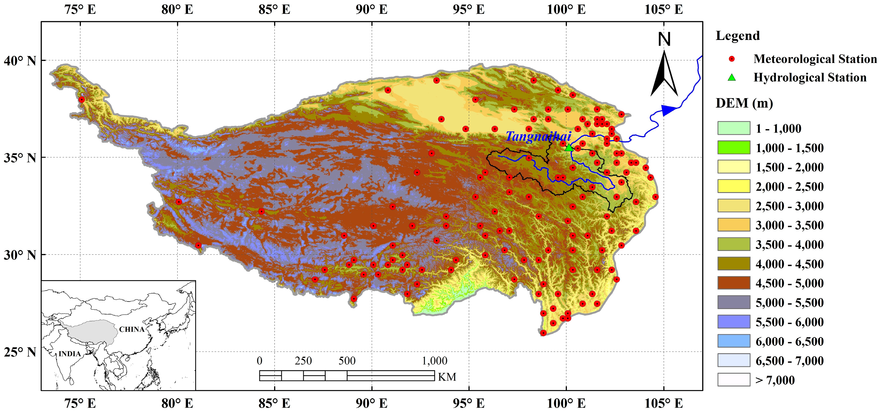
2.1. Study Area
2.2. Satellite Data
2.3. Ground Gauge Data
2.4. Geographical Data
3. Methodology
3.1. Verification Metrics
3.2. Hydrological Model
4. Results and Discussion
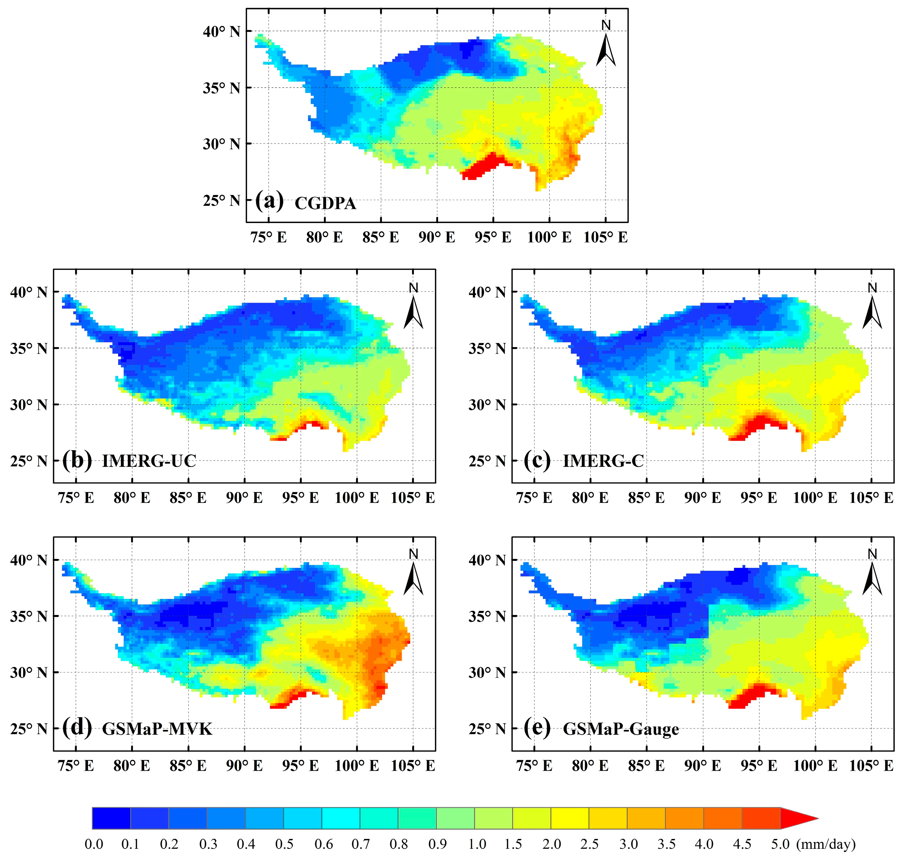
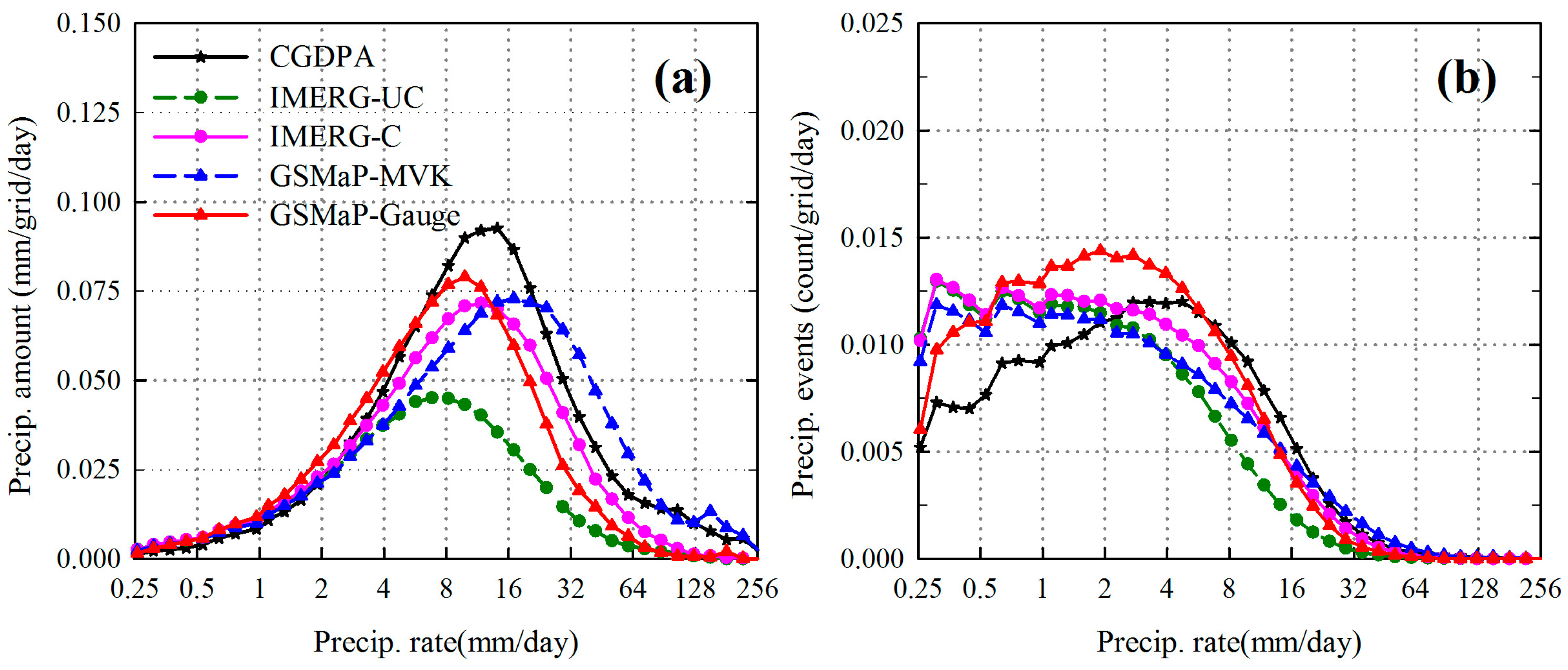
4.1. Rainfall Characteristics of the TP
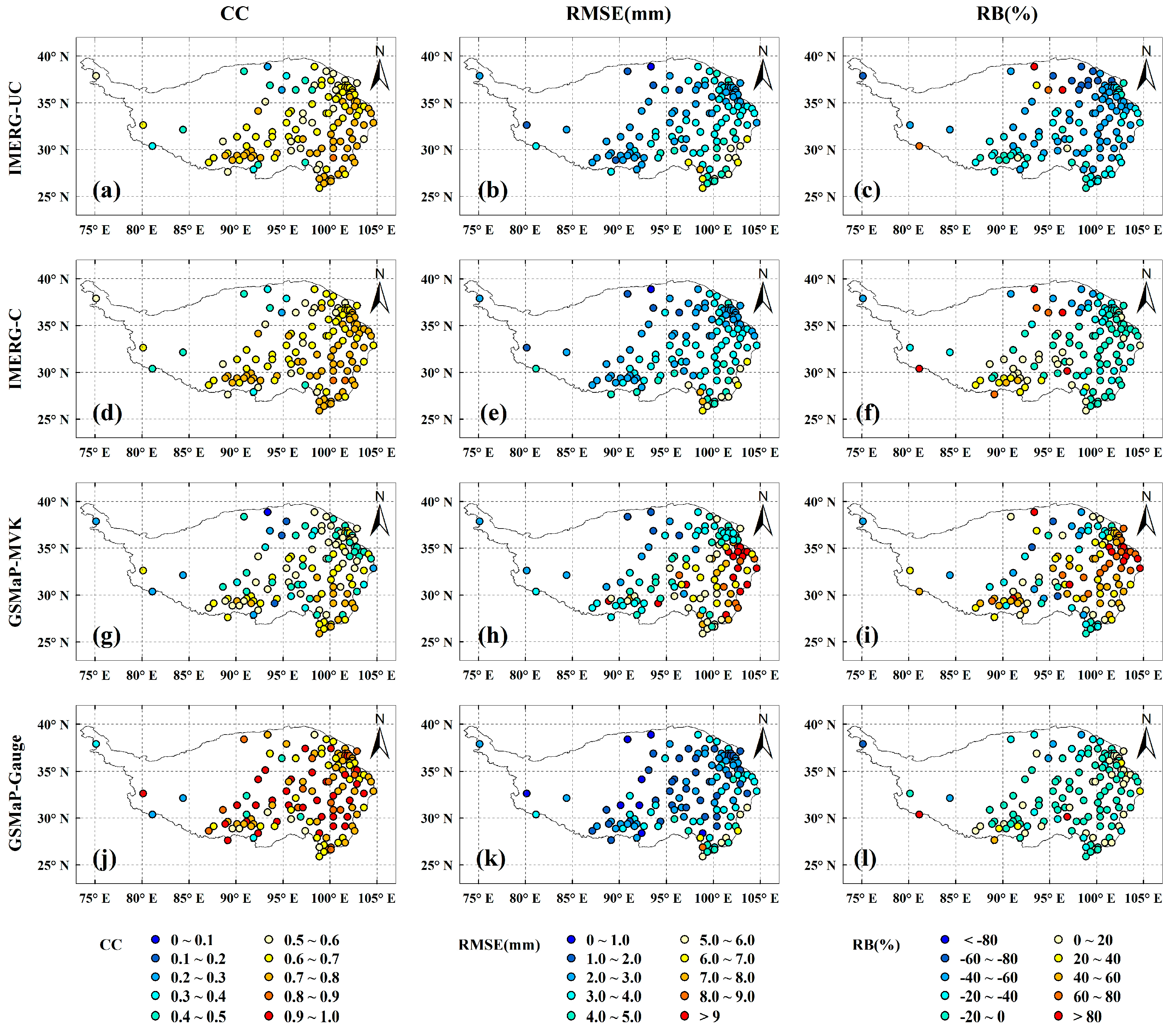
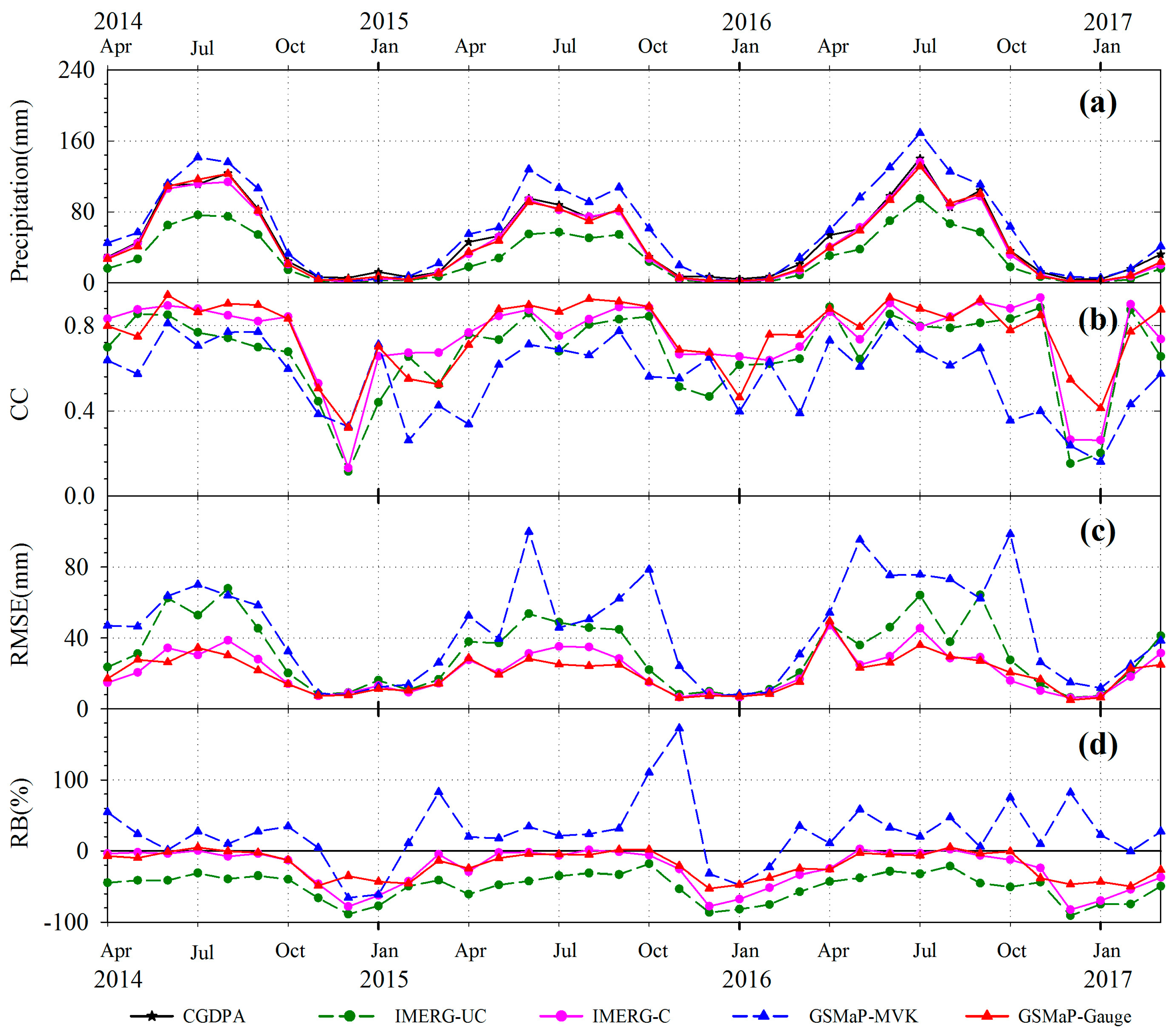
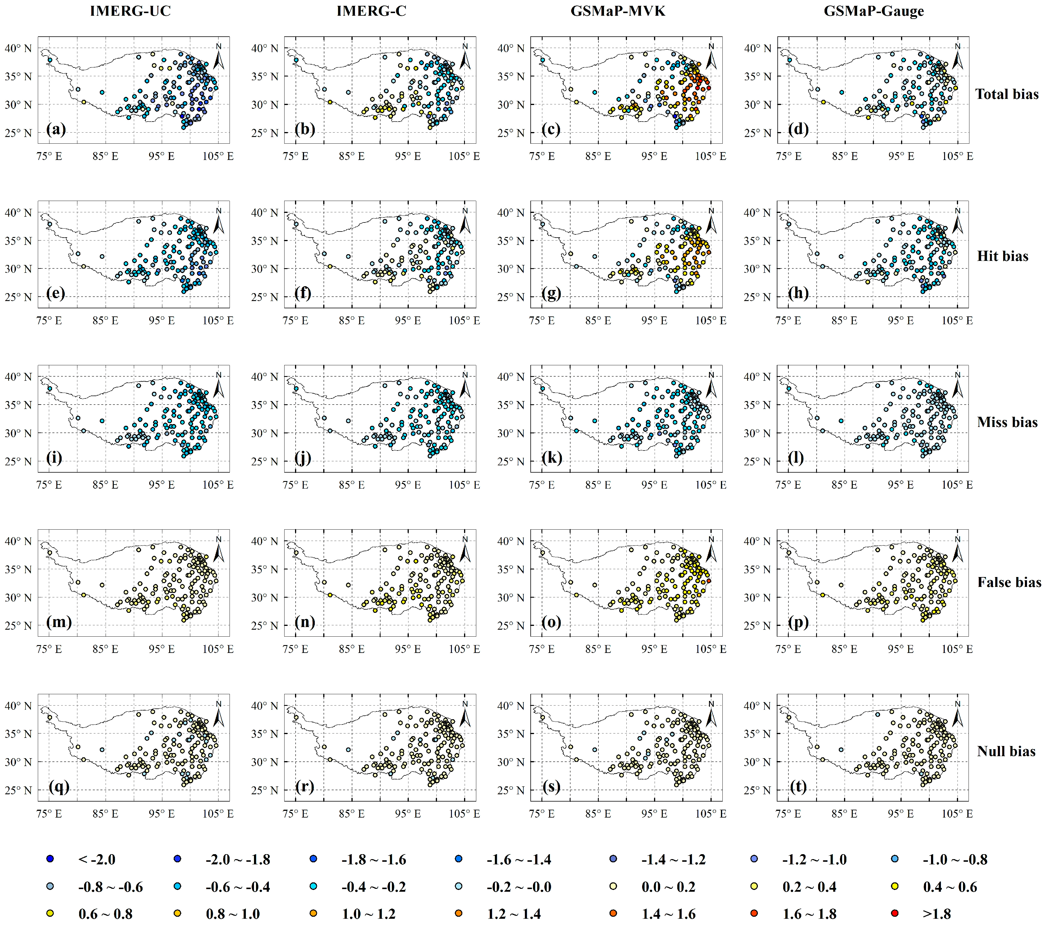
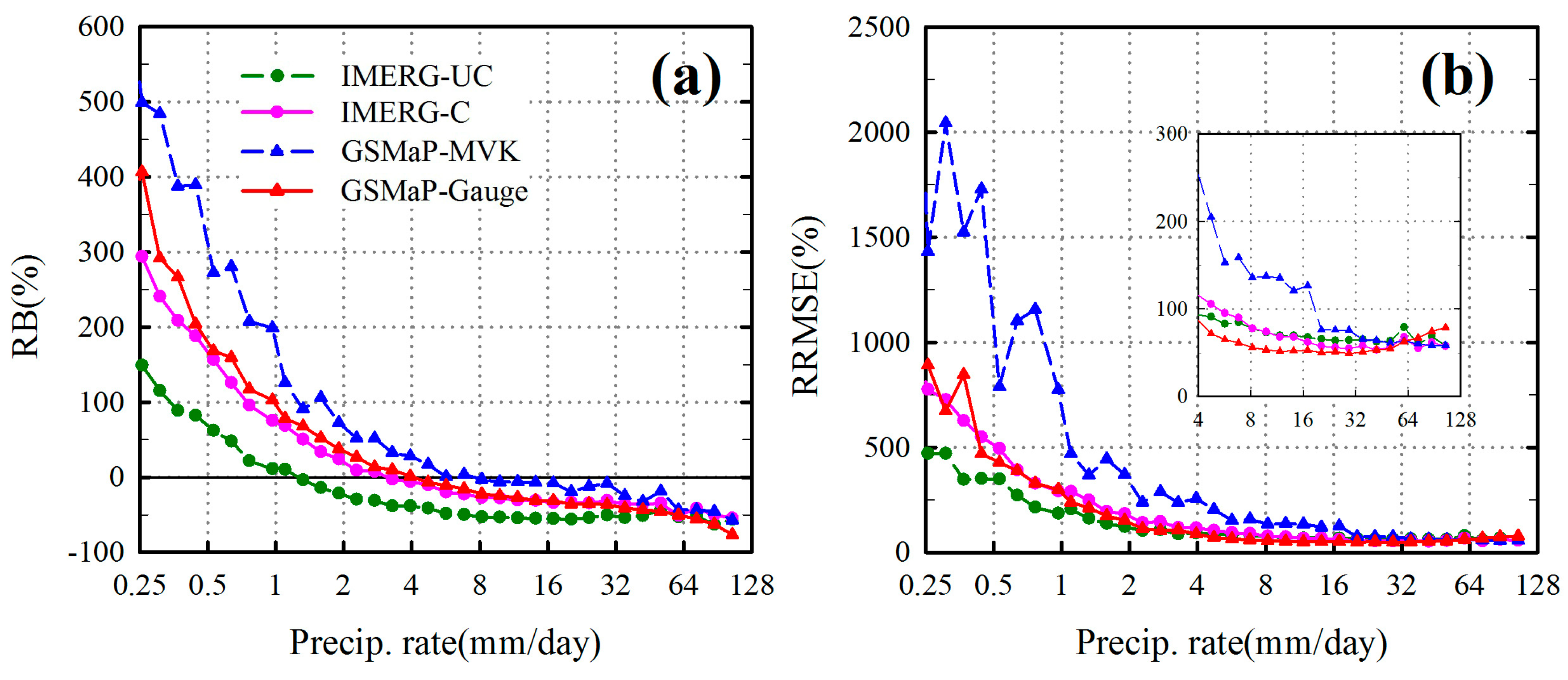
4.2. Statistical Performance of Satellite Precipitation Estimates
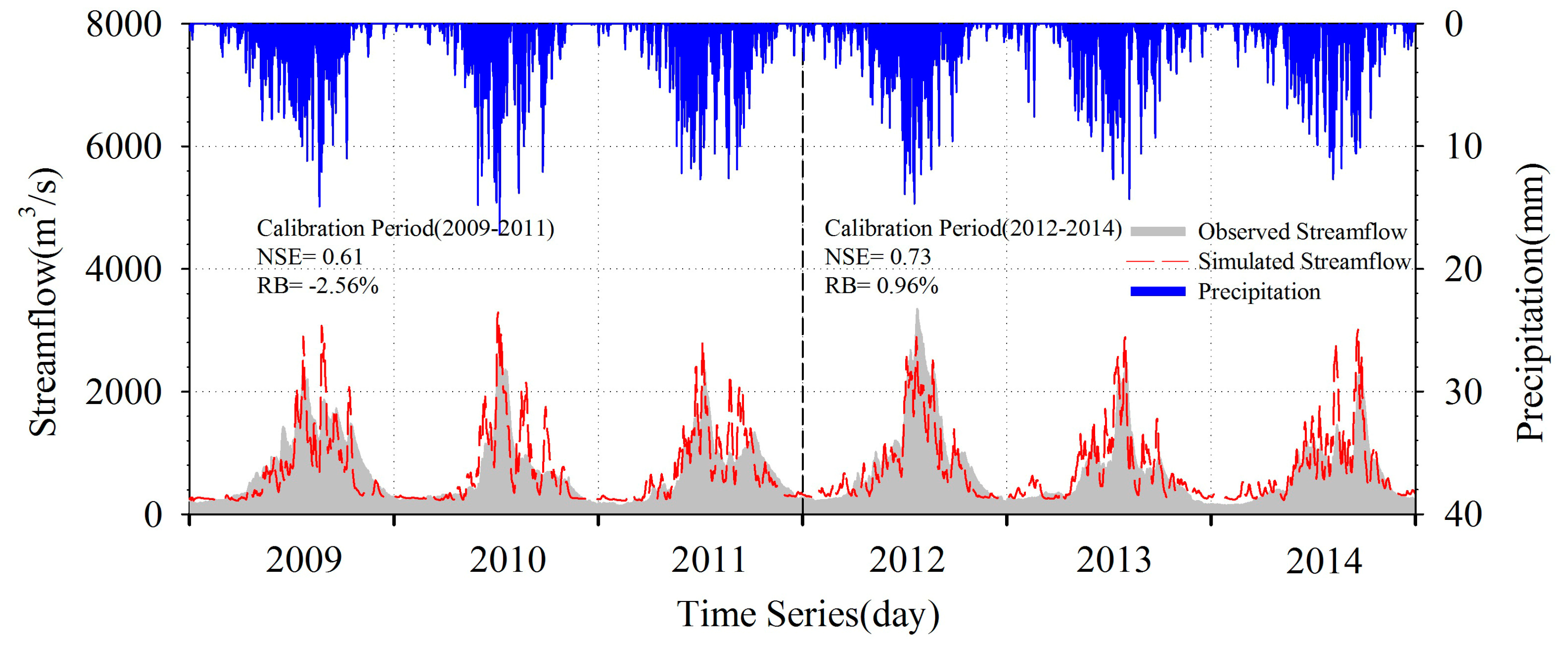
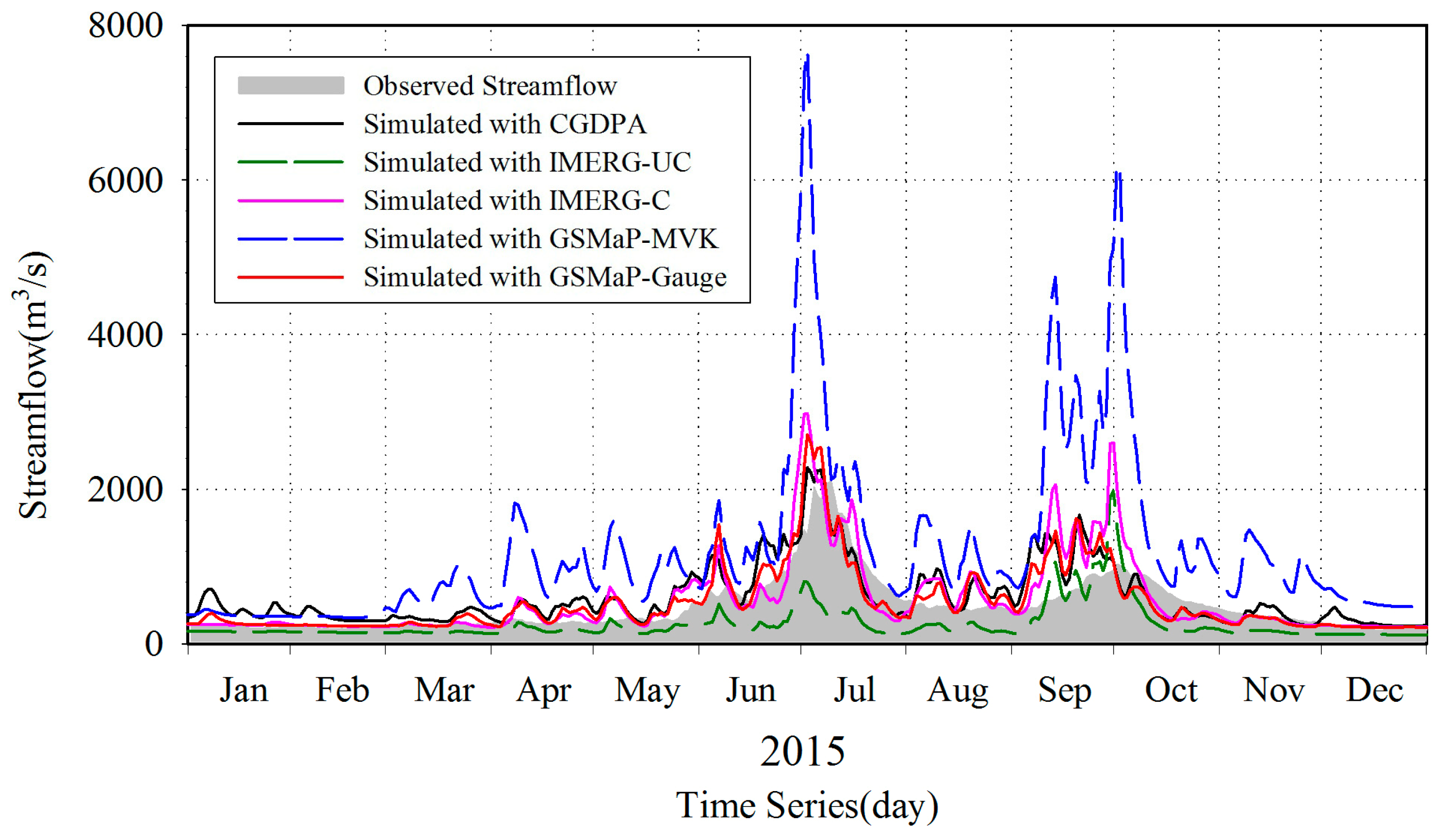
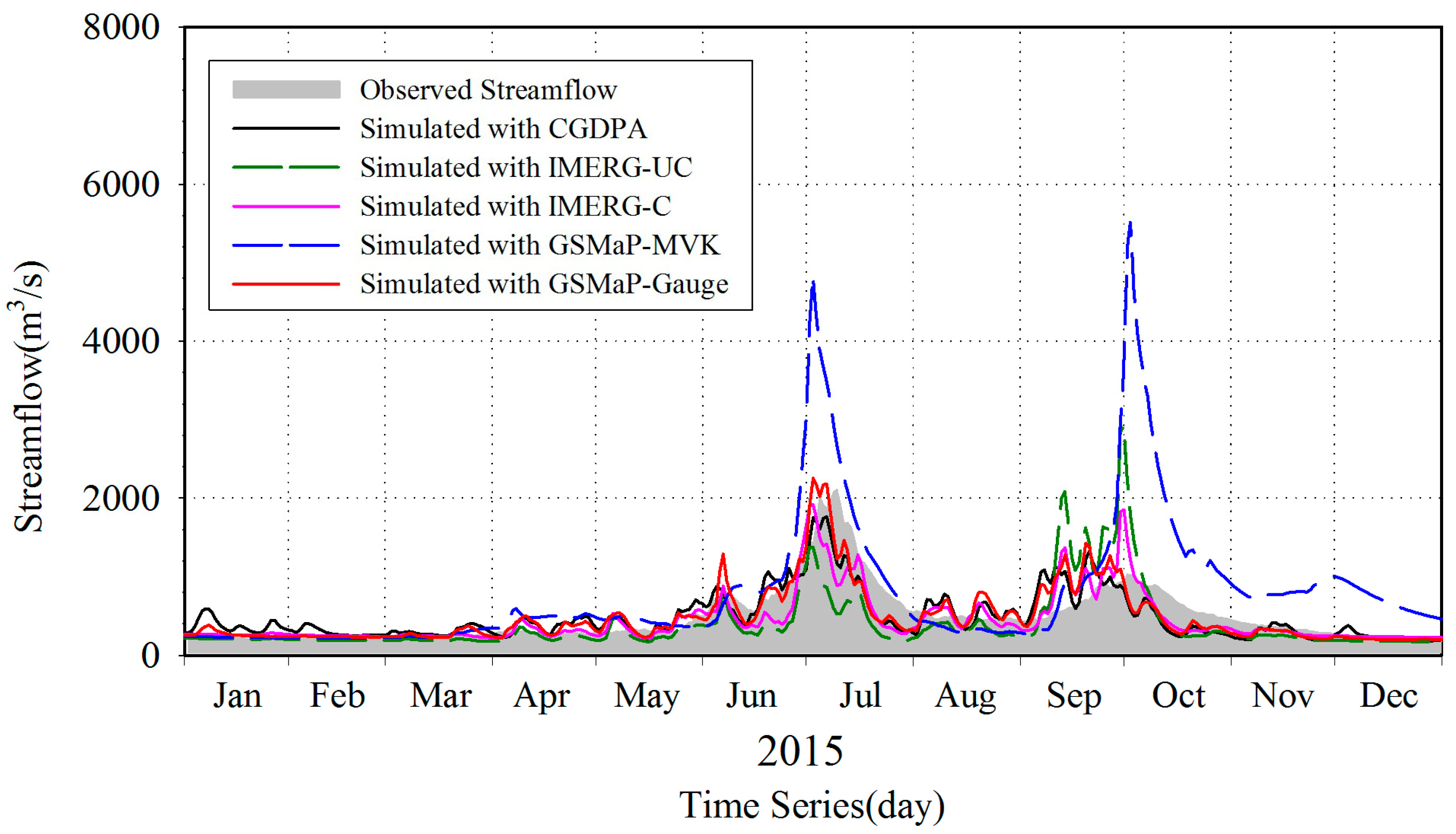
4.3. Hydrological Evaluation of Satellite Precipitation Estimates
5. Conclusions and Recommendations
Author Contributions
Funding
Acknowledgments
Conflicts of Interest
References
- Allen, M.R.; Ingram, W.J. Constraints on future changes in climate and the hydrologic cycle. Nature 2002, 419, 224–232. [Google Scholar] [CrossRef] [PubMed]
- Michaelides, S.; Levizzani, V.; Anagnostou, E.; Bauer, P.; Kasparis, T.; Lane, J.E. Precipitation: Measurement, remote sensing, climatology and modeling. Atmos. Res. 2009, 94, 512–533. [Google Scholar] [CrossRef]
- Kidd, C.; Levizzani, V. Status of satellite precipitation retrievals. Hydrol. Earth Syst. Sci. 2011, 15, 1109–1116. [Google Scholar] [CrossRef]
- Behrangi, A.; Khakbaz, B.; Jaw, T.C.; AghaKouchak, A.; Hsu, K.; Sorooshian, S. Hydrologic evaluation of satellite precipitation products over a mid-size basin. J. Hydrol. 2011, 397, 225–237. [Google Scholar] [CrossRef]
- Anagnostou, E.N.; Maggioni, V.; Nikolopoulos, E.I.; Meskele, T.; Hossain, F.; Papadopoulos, A. Benchmarking high-resolution global satellite rainfall products to radar and rain-gauge rainfall estimates. IEEE Trans. Geosci. Remote Sens. 2010, 48, 1667–1683. [Google Scholar] [CrossRef]
- Qiu, J. The third pole. Nature 2008, 454, 393–396. [Google Scholar] [CrossRef] [PubMed]
- Tong, K.; Su, F.; Yang, D.; Hao, Z. Evaluation of satellite precipitation retrievals and their potential utilities in hydrologic modeling over the Tibetan Plateau. J. Hydrol. 2014, 519, 423–437. [Google Scholar] [CrossRef]
- Hossain, F.; Lettenmaier, D.P. Flood prediction in the future: Recognizing hydrologic issues in anticipation of the Global Precipitation Measurement mission. Water Resour. Res. 2006, 42, W11301. [Google Scholar] [CrossRef]
- Katsanos, D.; Retalis, A.; Tymvios, F.; Michaelides, S. Analysis of precipitation extremes based on satellite (CHIRPS) and in situ dataset over Cyprus. Nat. Hazards 2016, 83, 53–63. [Google Scholar] [CrossRef]
- Tang, G.; Zeng, Z.; Long, D.; Guo, X.; Yong, B.; Zhang, W.; Hong, Y. Statistical and hydrological comparisons between TRMM and GPM level-3 products over a midlatitude basin: Is day-1 IMERG a good successor for TMPA 3B42V7? J. Hydrometeorol. 2016, 17, 121–137. [Google Scholar] [CrossRef]
- Hsu, K.; Gao, X.; Sorooshian, S.; Gupta, H.V. Precipitation estimation from remotely sensed information using artificial neural networks. J. Appl. Meteorol. 1997, 36, 1176–1190. [Google Scholar] [CrossRef]
- Joyce, R.J.; Janowiak, J.E.; Arkin, P.A.; Xie, P. CMORPH: A method that produces global precipitation estimates from passive microwave and infrared data at high spatial and temporal resolution. J. Hydrometeorol. 2004, 5, 487–503. [Google Scholar] [CrossRef]
- Turk, F.J.; Miller, S.D. Toward improved characterization of remotely sensed precipitation regimes with MODIS/AMSR-E blended data techniques. IEEE Trans. Geosci. Rem. Sens. 2005, 43, 1059–1069. [Google Scholar] [CrossRef]
- Huffman, G.J.; Adler, R.F.; Bolvin, D.T.; Gu, G.; Nelkin, E.G.; Bowman, K.P.; Hong, Y.; Stocker, E.F.; Wolff, D.B. The TRMM multisatellite precipitation analysis (TMPA): Quasi-global, multiyear, combined-sensor precipitation estimates at fine scales. J. Hydrometeorol. 2007, 8, 38–55. [Google Scholar] [CrossRef]
- Kubota, T.; Shige, S.; Hashizume, H.; Aonashi, K.; Takahashi, N.; Seto, S.; Hirose, M.; Takayabu, Y.N.; Nakagawa, K.; Iwanami, K.; et al. Global precipitation map using satellite-borne microwave radiometers by the GSMaP Project: Production and validation. IEEE Trans. Geosci. Remote Sens. 2007, 45, 2259–2275. [Google Scholar] [CrossRef]
- Hong, Y.; Adler, R.F.; Negri, A.; Huffman, G.J. Flood and landslide applications of near real-time satellite rainfall products. Nat. Hazards 2007, 43, 285–294. [Google Scholar] [CrossRef]
- Wu, H.; Adler, R.F.; Tian, Y.; Huffman, G.J.; Li, H.; Wang, J. Real-time global flood estimation using satellite-based precipitation and a coupled land surface and routing model. Water Resour. Res. 2014, 50, 2693–2717. [Google Scholar] [CrossRef]
- Yang, N.; Zhang, K.; Hong, Y.; Zhao, Q.; Huang, Q.; Xu, Y.; Xue, X.; Chen, S. Evaluation of the TRMM multisatellite precipitation analysis and its applicability in supporting reservoir operation and water resources management in Hanjiang basin, China. J. Hydrol. 2017, 549, 313–325. [Google Scholar] [CrossRef]
- Ebert, E.E.; Janowiak, J.E.; Kidd, C. Comparison of near-real-time precipitation estimates from satellite observations and numerical models. Bull. Am. Meteorol. Soc. 2007, 88, 47–64. [Google Scholar] [CrossRef]
- Maggioni, V.; Meyers, P.C.; Robinson, M.D. A review of merged high-resolution satellite precipitation product accuracy during the Tropical Rainfall Measuring Mission (TRMM) era. J. Hydrometeorol. 2016, 17, 1101–1117. [Google Scholar] [CrossRef]
- Tian, Y.; Peters-Lidard, C.D. A global map of uncertainties in satellite-based precipitation measurements. Geophys. Res. Lett. 2010, 37, L24407. [Google Scholar] [CrossRef]
- Yong, B.; Liu, D.; Gourley, J.J.; Tian, Y.; Huffman, G.J.; Ren, L.; Hong, Y. Global view of real-time TRMM multisatellite precipitation analysis: Implications for its successor global precipitation measurement mission. Bull. Am. Meteorol. Soc. 2015, 96, 283–296. [Google Scholar] [CrossRef]
- Hou, A.Y.; Kakar, R.K.; Neeck, S.; Azarbarzin, A.A.; Kummerow, C.D.; Kojima, M.; Oki, R.; Nakamura, K.; Iguchi, T. The global precipitation measurement mission. Bull. Am. Meteorol. Soc. 2014, 95, 701–722. [Google Scholar] [CrossRef]
- Skofronick-Jackson, G.; Petersen, W.A.; Berg, W.; Kidd, C.; Stocker, E.F.; Kirschbaum, D.B.; Kakar, R.; Braun, S.A.; Huffman, G.J.; Iguchi, T.; et al. The global precipitation measurement (GPM) mission for science and society. Bull. Am. Meteorol. Soc. 2017, 98, 1679–1695. [Google Scholar] [CrossRef]
- Skofronick-Jackson, G.; Berg, W.; Kidd, C.; Kirschbaum, D.B.; Petersen, W.A.; Huffman, G.J.; Takayabu, Y.N. Global Precipitation Measurement (GPM): Unified Precipitation Estimation from Space. In Remote Sensing of Clouds and Precipitation; Springer International Publishing AG: Cham, Switzerland, 2018; pp. 175–193. ISBN 978-3-319-72582-6. [Google Scholar]
- Huffman, G.J.; Bolvin, D.T.; Nelkin, E.J. Integrated Multi-satellitE Retrievals for GPM (IMERG) Technical Documentation. NASA/GSFC Code. Available online: https://pmm.nasa.gov/sites/default/files/document_files/IMERG_doc_180207.pdf (accessed on 6 September 2018).
- Skofronick-Jackson, G.; Huffman, G.; Petersen, W. Three Years of the Global Precipitation Measurement (GPM) Mission. Available online: https://ntrs.nasa.gov/archive/nasa/casi.ntrs.nasa.gov/20180000664.pdf (accessed on 6 September 2018).
- Gaona, M.R.; Overeem, A.; Leijnse, H.; Uijlenhoet, R. First-year evaluation of GPM rainfall over the Netherlands: IMERG day 1 final run (V03D). J. Hydrometeorol. 2016, 17, 2799–2814. [Google Scholar] [CrossRef]
- Tang, G.; Ma, Y.; Long, D.; Zhong, L.; Hong, Y. Evaluation of GPM Day-1 IMERG and TMPA Version-7 legacy products over Mainland China at multiple spatiotemporal scales. J. Hydrol. 2016, 533, 152–167. [Google Scholar] [CrossRef]
- Prakash, S.; Mitra, A.K.; AghaKouchak, A.; Liu, Z.; Norouzi, H.; Pai, D.S. A preliminary assessment of GPM-based multi-satellite precipitation estimates over a monsoon dominated region. J. Hydrol. 2016, 556, 865–876. [Google Scholar] [CrossRef]
- Sahlu, D.; Nikolopoulos, E.I.; Moges, S.A.; Anagnostou, E.N.; Hailu, D. First evaluation of the Day-1 IMERG over the upper Blue Nile Basin. J. Hydrometeor. 2016, 17, 2875–2882. [Google Scholar] [CrossRef]
- Gebregiorgis, A.S.; Kirstetter, P.E.; Hong, Y.E.; Gourley, J.J.; Huffman, G.J.; Petersen, W.A.; Xue, X.; Schwaller, M.R. To What Extent is the Day 1 GPM IMERG Satellite Precipitation Estimate Improved as Compared to TRMM TMPA-RT? J. Geophys. Res. Atmos. 2018, 123, 1694–1707. [Google Scholar] [CrossRef]
- Huffman, G.J.; Bolvin, D.T.; Nelkin, E.J. Day 1 IMERG Final Run Release Notes. NASA/GSFC: Greenbelt, MD, USA. Available online: https://pmm.nasa.gov/sites/default/files/document_files/IMERG_FinalRun_Day1_release_notes.pdf (accessed on 6 September 2018).
- Dezfuli, A.K.; Ichoku, C.M.; Huffman, G.J.; Mohr, K.I.; Selker, J.S.; Van De Giesen, N.; Hochreutener, R.; Annor, F.O. Validation of IMERG Precipitation in Africa. J. Hydrometeorol. 2017, 18, 2817–2825. [Google Scholar] [CrossRef]
- Oliveira, R.; Maggioni, V.; Vila, D.; Porcacchia, L. Using Satellite Error Modeling to Improve GPM-Level 3 Rainfall Estimates over the Central Amazon Region. Remote Sens. 2018, 10, 336. [Google Scholar] [CrossRef]
- Sharifi, E.; Steinacker, R.; Saghafian, B. Assessment of GPM-IMERG and other precipitation products against gauge data under different topographic and climatic conditions in Iran: Preliminary results. Remote Sens. 2016, 8, 135. [Google Scholar] [CrossRef]
- Chen, F.; Li, X. Evaluation of IMERG and TRMM 3B43 monthly precipitation products over mainland China. Remote Sens. 2016, 8, 472. [Google Scholar] [CrossRef]
- Asong, Z.E.; Razavi, S.; Wheater, H.S.; Wong, J.S. Evaluation of integrated multisatellite retrievals for GPM (IMERG) over southern Canada against ground precipitation observations: A preliminary assessment. J. Hydrometeorol. 2017, 18, 1033–1050. [Google Scholar] [CrossRef]
- Foelsche, U.; Kirchengast, G.; Fuchsberger, J.; Tan, J.; Petersen, W.A. Evaluation of GPM IMERG Early, Late, and Final rainfall estimates using WegenerNet gauge data in southeastern Austria. Hydrol. Earth Syst. Sci. 2017, 21, 6559–6572. [Google Scholar] [CrossRef]
- Huffman, G.J.; Bolvin, D.T.; Nelkin, E.J.; Stocker, E.F.; Tan, J. V05 IMERG Final Run Release Notes; NASA Goddard Earth Sciences Data and Information Services Center: Greenbelt, MD, USA, 2018. Available online: https://pmm.nasa.gov/sites/default/files/document_files/IMERG_FinalRun_V05_release_notes-rev3.pdf (accessed on 6 September 2018).
- Kubota, T.; Aonashi, K.; Ushio, T.; Shige, S.; Takayabu, Y.N.; Arai, Y.; Tashima, T.; Kachi, M.; Oki, R. Recent progress in global satellite mapping of precipitation (GSMaP) product. In Proceedings of the 2017 IEEE International Geoscience and Remote Sensing Symposium (IGARSS), Fort Worth, TX, USA, 23–28 July 2017; pp. 2712–2715. [Google Scholar] [CrossRef]
- Immerzeel, W.W.; Van Beek, L.P.H.; Bierkens, M.F.P. Climate change will affect the Asian water towers. Science 2010, 328, 1382–1385. [Google Scholar] [CrossRef]
- Guo, D.; Wang, H. The significant climate warming in the northern Tibetan Plateau and its possible causes. Int. J. Climatol. 2012, 32, 1775–1781. [Google Scholar] [CrossRef]
- Tong, K.; Su, F.; Yang, D.; Zhang, L.; Hao, Z. Tibetan Plateau precipitation as depicted by gauge observations, reanalyses and satellite retrievals. Int. J. Climatol. 2014, 34, 265–285. [Google Scholar] [CrossRef]
- Rees, H.G.; Collins, D.N. Regional differences in response of flow in glacier-fed Himalayan rivers to climatic warming. Hydrol. Process. 2006, 20, 1493–1517. [Google Scholar] [CrossRef]
- Cui, X.; Graf, H.F. Recent land cover changes on the Tibetan Plateau: A review. Clim. Chang. 2009, 94, 47–61. [Google Scholar] [CrossRef]
- Huffman, G.J.; Bolvin, D.T.; Braithwaite, D.; Hsu, K.; Joyce, R.; Kidd, C.; Nelkin, E.J.; Sorooshian, S.; Tan, J.; Xie, P. NASA Global Precipitation Measurement Integrated MultisatellitE Retrievals for GPM (IMERG). Algorithm Theoretical Basis Doc., Version 5.2. Available online: https://pmm.nasa.gov/sites/default/files/document_files/IMERG_ATBD_V5.2_0.pdf (accessed on 6 September 2018).
- Tan, J.; Petersen, W.A.; Kirstetter, P.E.; Tian, Y. Performance of IMERG as a function of spatiotemporal scale. J. Hydrometeorol. 2017, 18, 307–319. [Google Scholar] [CrossRef] [PubMed]
- Zhu, Z.; Yong, B.; Ke, L.; Wang, G.; Ren, L.; Chen, X. Tracing the Error Sources of Global Satellite Mapping of Precipitation for GPM (GPM-GSMaP) Over the Tibetan Plateau, China. IEEE J. Sel. Top. Appl. Earth Obs. Remote Sens. 2018, 11, 2181–2191. [Google Scholar] [CrossRef]
- Duan, Z.; Liu, J.; Tuo, Y.; Chiogna, G.; Disse, M. Evaluation of eight high spatial resolution gridded precipitation products in Adige Basin (Italy) at multiple temporal and spatial scales. Sci. Total Environ. 2016, 573, 1536–1553. [Google Scholar] [CrossRef] [PubMed]
- Ushio, T.; Sasashige, K.; Kubota, T.; Shige, S.; Okamoto, K.I.; Aonashi, K.; Inoue, T.; Takahashi, N.; Iguchi, T.; Kachi, M.; et al. A Kalman filter approach to the Global Satellite Mapping of Precipitation (GSMaP) from combined passive microwave and infrared radiometric data. J. Meteorol. Soc. Jpn. 2009, 87a, 137–151. [Google Scholar] [CrossRef]
- Xie, P.; Chen, M.; Yang, S.; Yatagai, A.; Hayasaka, T.; Fukushima, Y.; Liu, C. A gauge-based analysis of daily precipitation over East Asia. J. Hydrometeorol. 2007, 8, 607–626. [Google Scholar] [CrossRef]
- Omranian, E.; Sharif, H.O. Evaluation of the Global Precipitation Measurement (GPM) satellite rainfall products over the lower Colorado River basin, Texas. J. Am. Water Resour. Assoc. 2018. [Google Scholar] [CrossRef]
- Shen, Y.; Xiong, A.; Wang, Y.; Xie, P. Performance of high-resolution satellite precipitation products over China. J. Geophys. Res. Atmos. 2010, 115. [Google Scholar] [CrossRef]
- Guo, H.; Chen, S.; Bao, A.; Behrangi, A.; Hong, Y.; Ndayisaba, F.; Hu, J.; Stepanian, P.M. Early assessment of integrated multi-satellite retrievals for global precipitation measurement over China. Atmos. Res. 2016, 176, 121–133. [Google Scholar] [CrossRef]
- Shen, Y.; Xiong, A. Validation and comparison of a new gauge-based precipitation analysis over mainland China. Int. J. Climatol. 2016, 36, 252–265. [Google Scholar] [CrossRef]
- Zhao, H.; Yang, S.; You, S.; Huang, Y.; Wang, Q.; Zhou, Q. Comprehensive evaluation of two successive V3 and V4 IMERG Final Run precipitation products over mainland China. Remote Sens. 2017, 10, 34. [Google Scholar] [CrossRef]
- FAO. Food and Agriculture Association: Digital Soil Map of the World and Derived Soil Properties, Land and Water Digital Media Series; CD-ROM: Rome, Italy, 2003. [Google Scholar]
- Hansen, M.C.; DeFries, R.S.; Townshend, J.R.G.; Sohlberg, R. Global land cover classification at 1 km resolution using a classification tree approach. Int. J. Remote Sens. 2000, 21, 1331–1364. [Google Scholar] [CrossRef]
- Liang, X.; Lettenmaier, D.P.; Wood, E.F.; Burges, S.J. A simple hydrologically based model of land surface water and energy fluxes for GSMs. J. Geophys. Res. Atmos. 1994, 99, 14415–14428. [Google Scholar] [CrossRef]
- Liang, X.; Wood, E.F.; Lettenmaier, D.P. Surface soil moisture parameterization of the VIC-2L model: Evaluation and modification. Glob. Planet. Chang. 1996, 13, 195–206. [Google Scholar] [CrossRef]
- Gao, H.; Tang, Q.; Shi, X.; Zhu, C.; Bohn, T.; Su, F.; Sheffield, J.; Pan, M.; Lettenmaier, D.; Wood, E.F. Water Budget Record from Variable Infiltration Capacity (VIC) Model Algorithm Theoretical Basis Document, Algorithm Theoretical Basis Document for Terrestrial Water Cycle Data Records. Available online: http://dynamo.hydro.washington.edu/SurfaceWaterGroup/Publications/Water_Cycle_MEaSUREs_ATBD_VICmodel_submit.doc (accessed on 6 September 2018).
- Nijssen, B.; Lettenmaier, D.P.; Liang, X.; Wetzel, S.W.; Wood, E.F. Streamflow simulation for continental-scale river basins. Water Resour. Res. 1997, 33, 711–724. [Google Scholar] [CrossRef]
- Xie, Z.; Yuan, F.; Duan, Q.; Zheng, J.; Liang, M.; Chen, F. Regional parameter estimation of the VIC land surface model: Methodology and application to river basins in China. J. Hydrometeorol. 2007, 8, 447–468. [Google Scholar] [CrossRef]
- Su, F.; Hong, Y.; Lettenmaier, D.P. Evaluation of TRMM multisatellite precipitation analysis (TMPA) and its utility in hydrologic prediction in the La Plata basin. J. Hydrometeorol. 2008, 9, 622–640. [Google Scholar] [CrossRef]
- Yong, B.; Hong, Y.; Ren, L.; Gourley, J.; Huffman, G.; Chen, X.; Wang, W.; Khan, S. Hydrologic evaluation of multisatellite precipitation analysis standard precipitation products in basins beyond its inclined latitude band: A case study in Laohahe basin, China. Water Resour. Res. 2010, 46, W07542. [Google Scholar] [CrossRef]
- Sun, R.; Yuan, H.; Liu, X.; Jiang, X. Evaluation of the latest satellite–gauge precipitation products and their hydrologic applications over the Huaihe River basin. J. Hydrol. 2016, 536, 302–319. [Google Scholar] [CrossRef]
- Ma, Y.; Tang, G.; Long, D.; Yong, B.; Zhong, L.; Wan, W.; Hong, Y. Similarity and error intercomparison of the GPM and its predecessor-TRMM Multisatellite Precipitation Analysis using the best available hourly gauge network over the Tibetan Plateau. Remote Sens. 2016, 8, 569. [Google Scholar] [CrossRef]
- Tian, Y.; Peters-Lidard, C.D.; Eylander, J.B.; Joyce, R.J.; Huffman, G.J.; Adler, R.F.; Hsu, K.; Turk, F.J.; Garcia, M.; Zeng, J. Component analysis of errors in satellite-basd precipitation estimates. J. Geophys. Res. Atmos. 2009, 114, D24101. [Google Scholar] [CrossRef]
- Li, Z.; Yang, D.; Hong, Y. Multi-scale evaluation of high-resolution multi-sensor blended global precipitation products over the Yangtze River. J. Hydrol. 2013, 500, 157–169. [Google Scholar] [CrossRef]
- Kim, K.; Park, J.; Baik, J.; Choi, M. Evaluation of topographical and seasonal feature using GPM IMERG and TRMM 3B42 over Far-East Asia. Atmos. Res. 2017, 187, 95–105. [Google Scholar] [CrossRef]
- Ning, S.W.; Wang, J.; Jin, J.L.; Ishidaira, H. Assessment of the latest GPM-Era high-resolution satellite precipitation products by comparison with Observation Gauge Data over the Chinese Mainland. Water 2016, 8, 481. [Google Scholar] [CrossRef]
- Yong, B.; Chen, B.; Tian, Y.; Yu, Z.; Hong, Y. Error-component analysis of TRMM-based multi-satellite precipitation estimates over mainland China. Remote Sens. 2016, 8, 440. [Google Scholar] [CrossRef]
- Su, J.; Lü, H.; Zhu, Y.; Wang, X.; Wei, G. Component Analysis of Errors in Four GPM-Based Precipitation Estimations over Mainland China. Remote Sens. 2018, 10, 1420. [Google Scholar] [CrossRef]
- Wang, D.; Wang, X.; Liu, L.; Wang, D.; Huang, H.; Pan, C. Evaluation of TMPA 3B42V7, GPM IMERG and CMPA precipitation estimates in Guangdong Province, China. Int. J. Climatol. 2018. [Google Scholar] [CrossRef]
- Omranian, E.; Sharif, H.; Tavakoly, A. How well can global precipitation measurement (GPM) capture hurricanes? case study: Hurricane Harvey. Remote Sens. 2018, 10, 1150. [Google Scholar] [CrossRef]
- Yong, B.; Wang, J.; Ren, L.; You, Y.; Xie, P.; Hong, Y. Evaluating four multisatellite precipitation estimates over the Diaoyu Islands during Typhoon seasons. J. Hydrometeorol. 2016, 17, 1623–1641. [Google Scholar] [CrossRef]
- Xue, X.; Hong, Y.; Limaye, A.S.; Gourley, J.J.; Huffman, G.J.; Khan, S.I.; Dorji, C.; Chen, S. Statistical and hydrological evaluation of TRMM-based multi-satellite precipitation analysis over the Wangchu basin of Bhutan: Are the latest satellite precipitation products 3B42V7 ready for use in ungauged basins? J. Hydrol. 2013, 499, 91–99. [Google Scholar] [CrossRef]
- Yuan, F.; Wang, B.; Shi, C.; Cui, W.; Zhao, C.; Liu, Y.; Ren, L.; Zhang, L.; Zhu, Y.; Chen, T.; et al. Evaluation of hydrological utility of IMERG Final Run V05 and TMPA 3B42V7 satellite precipitation products in the Yellow River source region, China. J. Hydrol. 2018. [Google Scholar] [CrossRef]
- Maggioni, V.; Massari, C. On the performance of satellite precipitation products in riverine flood modeling: A review. J. Hydrol. 2018, 558, 214–224. [Google Scholar] [CrossRef]
- Jiang, S.; Ren, L.; Xu, C.Y.; Yong, B.; Yuan, F.; Liu, Y.; Yang, X.; Zeng, X. Statistical and hydrological evaluation of the latest Integrated Multi-satellitE Retrievals for GPM (IMERG) over a midlatitude humid basin in South China. Atmos. Res. 2018, 214, 418–429. [Google Scholar] [CrossRef]
- Prakash, S.; Kumar, M.R.; Mathew, S.; Venkatesan, R. How accurate are satellite estimates of precipitation over the north Indian Ocean? Theor. Appl. Climatol. 2017, 134, 467–475. [Google Scholar] [CrossRef]


| Product | Temporal Resolution | Spatial Resolution | Start Time | Latency | Coverage | Corrected by Gauges |
|---|---|---|---|---|---|---|
| IMERG-UC | 0.5 h | 0.1° | 12 March 2014 | 3 months | 90°N–90°S | No |
| IMERG-C | 0.5 h | 0.1° | 12 March 2014 | 3 months | 90°N–90°S | Yes (GPCC monthly) |
| GSMaP-MVK | 1 h | 0.1° | 1 March 2014 | 3 days | 60°N–60°S | No |
| GSMaP-Gauge | 1 h | 0.1° | 1 March 2014 | 3 days | 60°N–60°S | Yes (CPC daily) |
| Statistic Index | Formula | Unit | Perfect Value |
|---|---|---|---|
| Correlation coefficient (CC) | - | 1 | |
| Root-mean-squared error (RMSE) | mm | 0 | |
| Mean error (ME) | mm | 0 | |
| Relative root-mean-squared error (RRMSE) | % | 0 | |
| Relative bias (RB) | % | 0 | |
| Probability of detection (POD) | - | 1 | |
| False alarm ratio (FAR) | - | 0 | |
| Frequency bias index (FBI) | - | 1 | |
| Equitable Threat Score (ETS) | - | 1 | |
| Nash–Sutcliffe coefficient of efficiency (NSE) | - | 1 |
| Season | Product | CC | RMSE (mm) | ME (mm) | RRMSE (%) | RB (%) | POD | FAR | FBI | ETS |
|---|---|---|---|---|---|---|---|---|---|---|
| Spring | IMERG-UC | 0.56 | 3.26 | −0.62 | 242.87 | −46.38 | 0.51 | 0.30 | 0.74 | 0.33 |
| IMERG-C | 0.61 | 3.17 | −0.18 | 236.01 | −13.60 | 0.64 | 0.38 | 1.03 | 0.36 | |
| GSMaP-MVK | 0.38 | 6.24 | 0.43 | 464.42 | 31.94 | 0.64 | 0.44 | 1.14 | 0.31 | |
| GSMaP-Gauge | 0.71 | 2.71 | −0.21 | 201.69 | −15.53 | 0.82 | 0.30 | 1.17 | 0.52 | |
| Summer | IMERG-UC | 0.67 | 5.15 | −1.26 | 139.24 | −34.02 | 0.72 | 0.22 | 0.93 | 0.39 |
| IMERG-C | 0.68 | 5.27 | −0.10 | 142.52 | −2.74 | 0.80 | 0.26 | 1.07 | 0.40 | |
| GSMaP-MVK | 0.59 | 8.01 | 0.86 | 216.56 | 23.16 | 0.78 | 0.27 | 1.08 | 0.37 | |
| GSMaP-Gauge | 0.76 | 4.36 | −0.08 | 117.87 | −2.03 | 0.91 | 0.24 | 1.20 | 0.50 | |
| Autumn | IMERG-UC | 0.66 | 3.18 | −0.57 | 218.98 | −39.09 | 0.60 | 0.25 | 0.81 | 0.41 |
| IMERG-C | 0.71 | 3.12 | −0.11 | 214.77 | −7.44 | 0.69 | 0.31 | 1.01 | 0.43 | |
| GSMaP-MVK | 0.44 | 6.96 | 0.52 | 478.63 | 35.58 | 0.70 | 0.37 | 1.12 | 0.39 | |
| GSMaP-Gauge | 0.77 | 2.67 | −0.06 | 183.5 | −4.41 | 0.87 | 0.27 | 1.19 | 0.57 | |
| Winter | IMERG-UC | 0.54 | 1.45 | −0.21 | 522.96 | −76.56 | 0.13 | 0.43 | 0.23 | 0.11 |
| IMERG-C | 0.58 | 1.39 | −0.17 | 500.66 | −62.17 | 0.19 | 0.54 | 0.42 | 0.14 | |
| GSMaP-MVK | 0.30 | 1.95 | −0.05 | 701.76 | −18.30 | 0.29 | 0.66 | 0.85 | 0.16 | |
| GSMaP-Gauge | 0.58 | 1.40 | −0.13 | 501.71 | −45.07 | 0.52 | 0.38 | 0.84 | 0.38 |
| Season | Product | H (%) | −M (%) | F (%) | N (%) | E = H − M + F + N (%) |
|---|---|---|---|---|---|---|
| Spring | IMERG-UC | −27.84 | −28.62 | 8.07 | 2.04 | −46.35 |
| IMERG-C | −13.73 | −19.75 | 16.66 | 3.24 | −13.58 | |
| GSMaP-MVK | 18.94 | −22.63 | 33.22 | 2.41 | 31.94 | |
| GSMaP-Gauge | −21.52 | −8.31 | 11.14 | 3.16 | −15.53 | |
| Summer | IMERG-UC | −28.70 | −12.31 | 6.36 | 0.62 | −34.03 |
| IMERG-C | −5.89 | −8.20 | 10.59 | 0.74 | −2.76 | |
| GSMaP-MVK | 18.45 | −10.12 | 13.99 | 0.85 | 23.17 | |
| GSMaP-Gauge | −9.47 | −3.26 | 9.49 | 1.20 | −2.04 | |
| Autumn | IMERG-UC | −26.67 | −20.41 | 6.69 | 1.30 | −39.09 |
| IMERG-C | −6.72 | −14.80 | 12.22 | 1.88 | −7.42 | |
| GSMaP-MVK | 19.75 | −15.31 | 28.57 | 2.57 | 35.58 | |
| GSMaP-Gauge | −11.85 | −5.85 | 11.28 | 2.00 | −4.42 | |
| Winter | IMERG-UC | −12.94 | −67.39 | 4.42 | −0.65 | −76.56 |
| IMERG-C | −13.16 | −60.48 | 9.31 | 2.19 | −62.14 | |
| GSMaP-MVK | −6.04 | −55.34 | 37.97 | 5.07 | −18.34 | |
| GSMaP-Gauge | −32.33 | −28.44 | 11.40 | 4.31 | −45.06 | |
| All Season | IMERG-UC | −27.46 | −19.59 | 6.71 | 1.01 | −39.33 |
| IMERG-C | −7.96 | −14.06 | 12.14 | 1.56 | −8.32 | |
| GSMaP-MVK | 17.89 | −15.59 | 22.09 | 1.72 | 26.11 | |
| GSMaP-Gauge | −13.35 | −5.84 | 10.30 | 1.90 | −6.99 |
| Product | CC | RMSE (mm) | RB (%) | |
|---|---|---|---|---|
| Grid scale | IMERG-UC | 0.57 | 3.10 | −46.65 |
| IMERG-C | 0.61 | 3.30 | −12.05 | |
| GSMaP-MVK | 0.52 | 5.78 | 59.25 | |
| GSMaP-Gauge | 0.75 | 2.41 | −3.19 | |
| Basin scale | IMERG-UC | 0.74 | 1.65 | −46.07 |
| IMERG-C | 0.79 | 1.60 | −12.19 | |
| GSMaP-MVK | 0.74 | 2.70 | 48.01 | |
| GSMaP-Gauge | 0.93 | 0.82 | −4.90 |
| Time Scales | Precipitation Products | Benchmarking Calibration | Product-Specific Calibration | ||||
|---|---|---|---|---|---|---|---|
| NSE | RB (%) | RMSE (m3/s) | NSE | RB (%) | RMSE (m3/s) | ||
| Daily | CGDPA | 0.41 | 26.39 | 274.05 | 0.63 | 0.55 | 217.11 |
| IMERG-UC | −0.12 | −46.00 | 377.46 | −0.08 | −18.96 | 370.33 | |
| IMERG-C | 0.18 | 17.97 | 323.77 | 0.62 | −7.26 | 220.87 | |
| GSMaP-MVK | −9.85 | 151.97 | 1175.70 | −2.93 | 66.73 | 707.77 | |
| GSMaP-Gauge | 0.53 | 11.64 | 243.91 | 0.67 | 0.13 | 205.56 | |
| Monthly | CGDPA | 0.53 | 26.48 | 214.93 | 0.70 | 0.62 | 168.61 |
| IMERG-UC | −0.17 | −45.96 | 333.21 | 0.15 | −18.90 | 286.48 | |
| IMERG-C | 0.63 | 18.05 | 191.45 | 0.76 | −7.19 | 150.74 | |
| GSMaP-MVK | −6.88 | 152.16 | 876.17 | −1.85 | 66.85 | 518.21 | |
| GSMaP-Gauge | 0.74 | 11.73 | 160.89 | 0.79 | 0.21 | 140.43 | |
© 2018 by the authors. Licensee MDPI, Basel, Switzerland. This article is an open access article distributed under the terms and conditions of the Creative Commons Attribution (CC BY) license (http://creativecommons.org/licenses/by/4.0/).
Share and Cite
Lu, D.; Yong, B. Evaluation and Hydrological Utility of the Latest GPM IMERG V5 and GSMaP V7 Precipitation Products over the Tibetan Plateau. Remote Sens. 2018, 10, 2022. https://doi.org/10.3390/rs10122022
Lu D, Yong B. Evaluation and Hydrological Utility of the Latest GPM IMERG V5 and GSMaP V7 Precipitation Products over the Tibetan Plateau. Remote Sensing. 2018; 10(12):2022. https://doi.org/10.3390/rs10122022
Chicago/Turabian StyleLu, Dekai, and Bin Yong. 2018. "Evaluation and Hydrological Utility of the Latest GPM IMERG V5 and GSMaP V7 Precipitation Products over the Tibetan Plateau" Remote Sensing 10, no. 12: 2022. https://doi.org/10.3390/rs10122022
APA StyleLu, D., & Yong, B. (2018). Evaluation and Hydrological Utility of the Latest GPM IMERG V5 and GSMaP V7 Precipitation Products over the Tibetan Plateau. Remote Sensing, 10(12), 2022. https://doi.org/10.3390/rs10122022