Monitoring Land-Use/Land-Cover Changes at a Provincial Large Scale Using an Object-Oriented Technique and Medium-Resolution Remote-Sensing Images


Abstract
1. Introduction
2. Materials
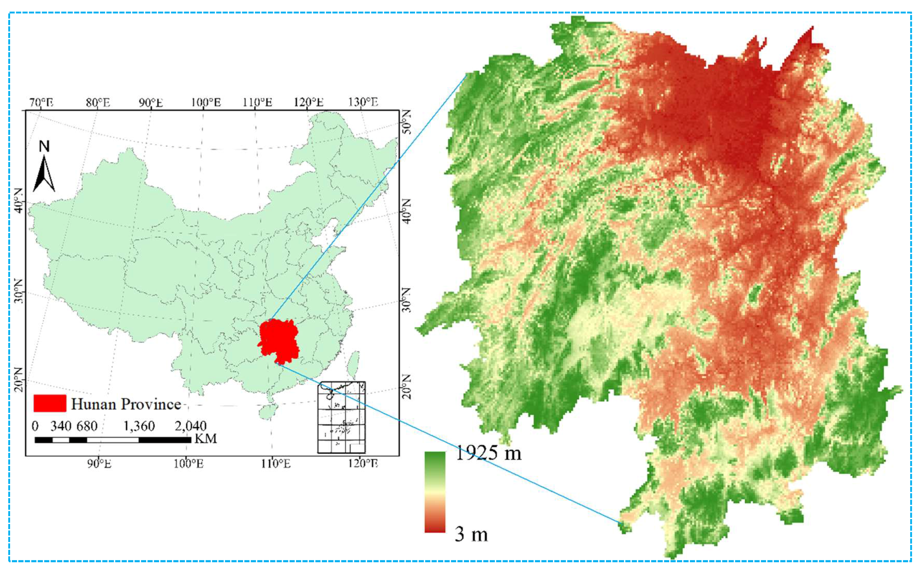
2.1. Study Area
2.2. Satellite Imagery
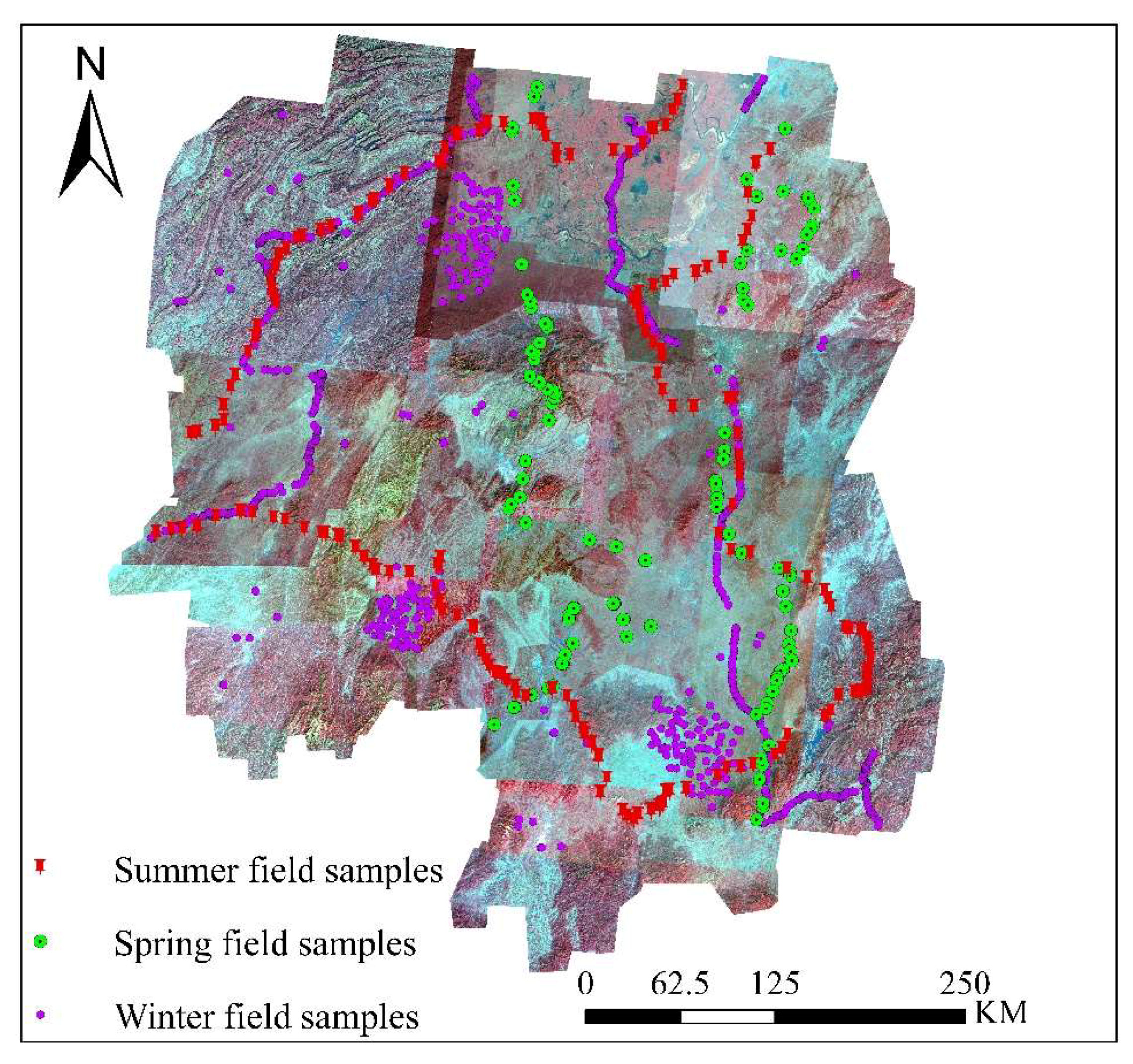
2.3. Field Data
2.4. Reference Data
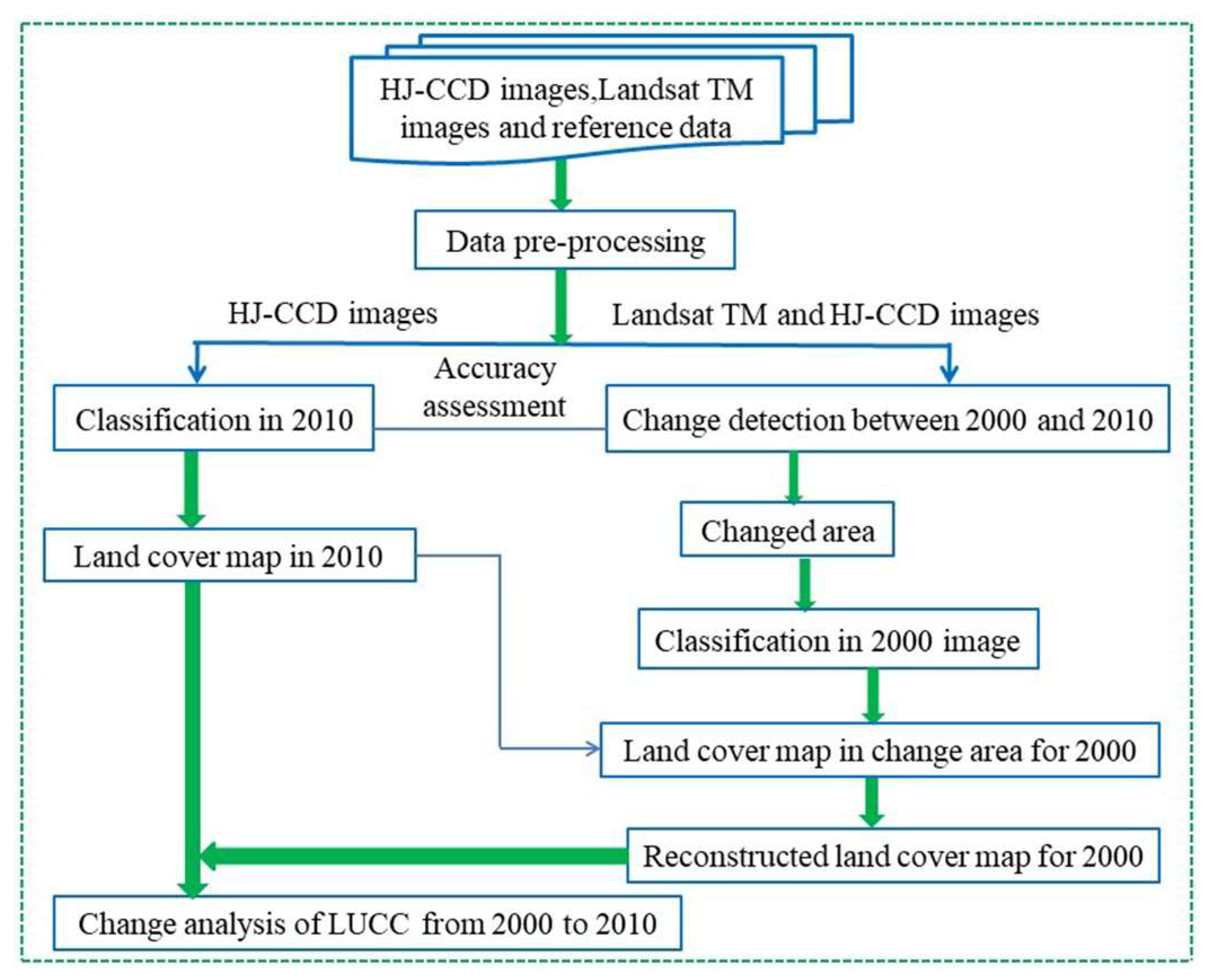
3. Methods
3.1. Data Preprocessing
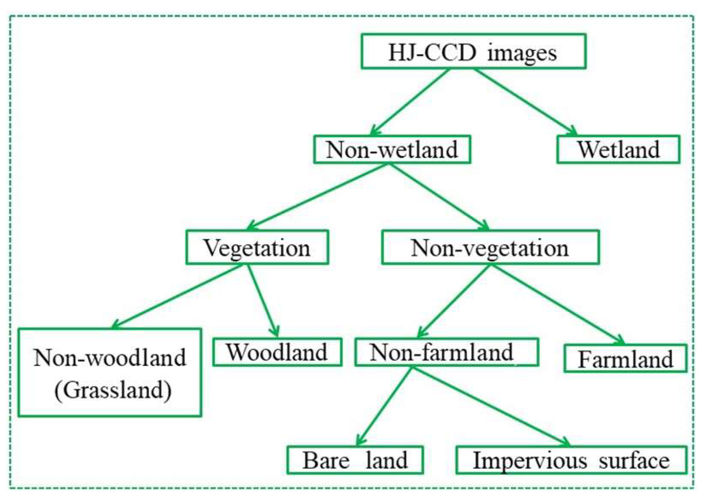
3.2. Object-Based Image Analysis Technique
3.2.1. Image Segmentation
3.2.2. 2010 Land Cover Classification
3.2.3. Land Cover Change Detection
3.3. Land Cover Map Reconstruction for 2000
3.4. Accuracy Verification
3.5. Speed and Amplitude of Land Cover Change
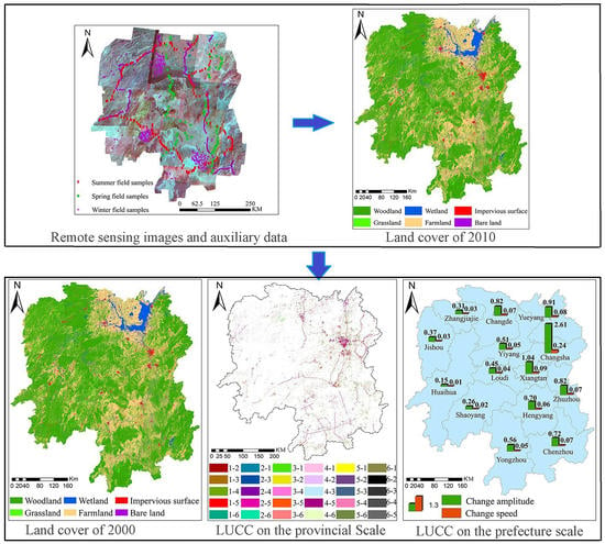
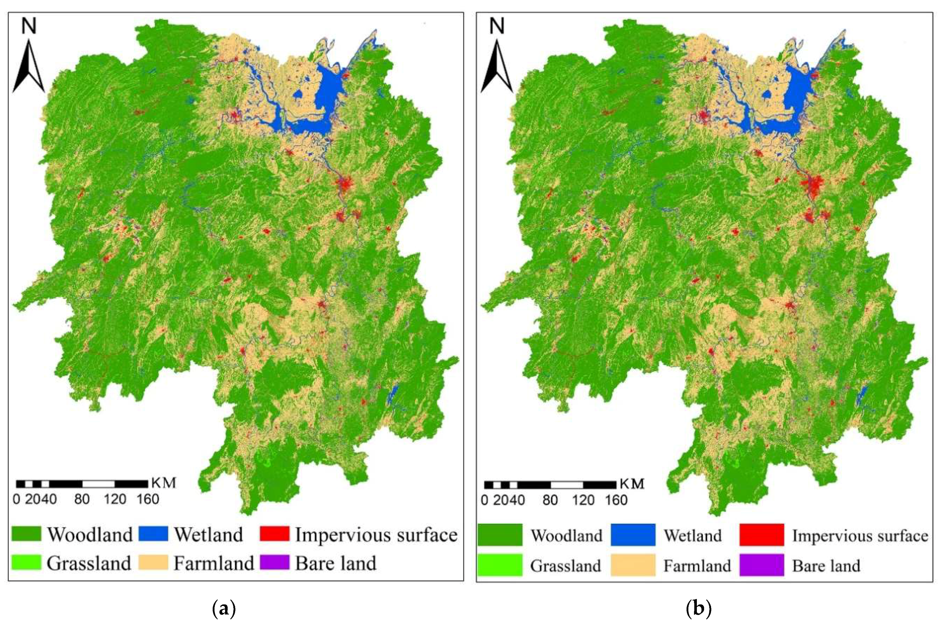
4. Results
4.1. Classification Results and Accuracy
4.2. Land Cover Pattern in Hunan Province
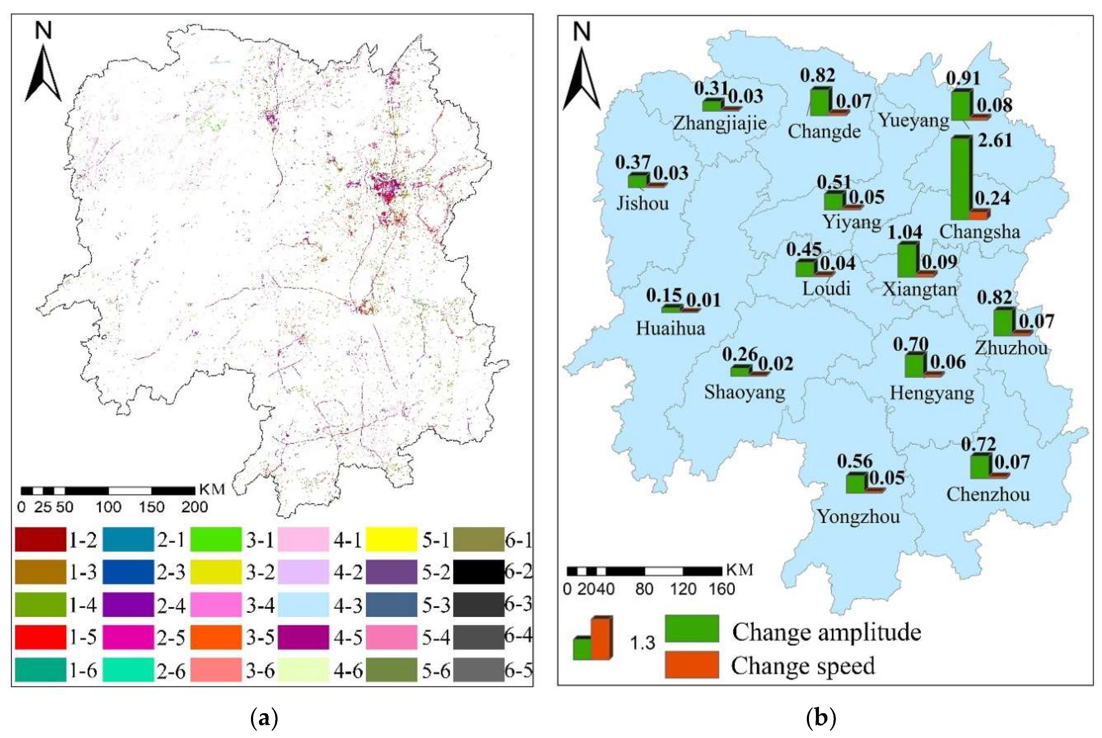
4.3. Land Cover Change in 2000–2010
4.1.1. Change Characteristics
4.1.2. Transfer Process
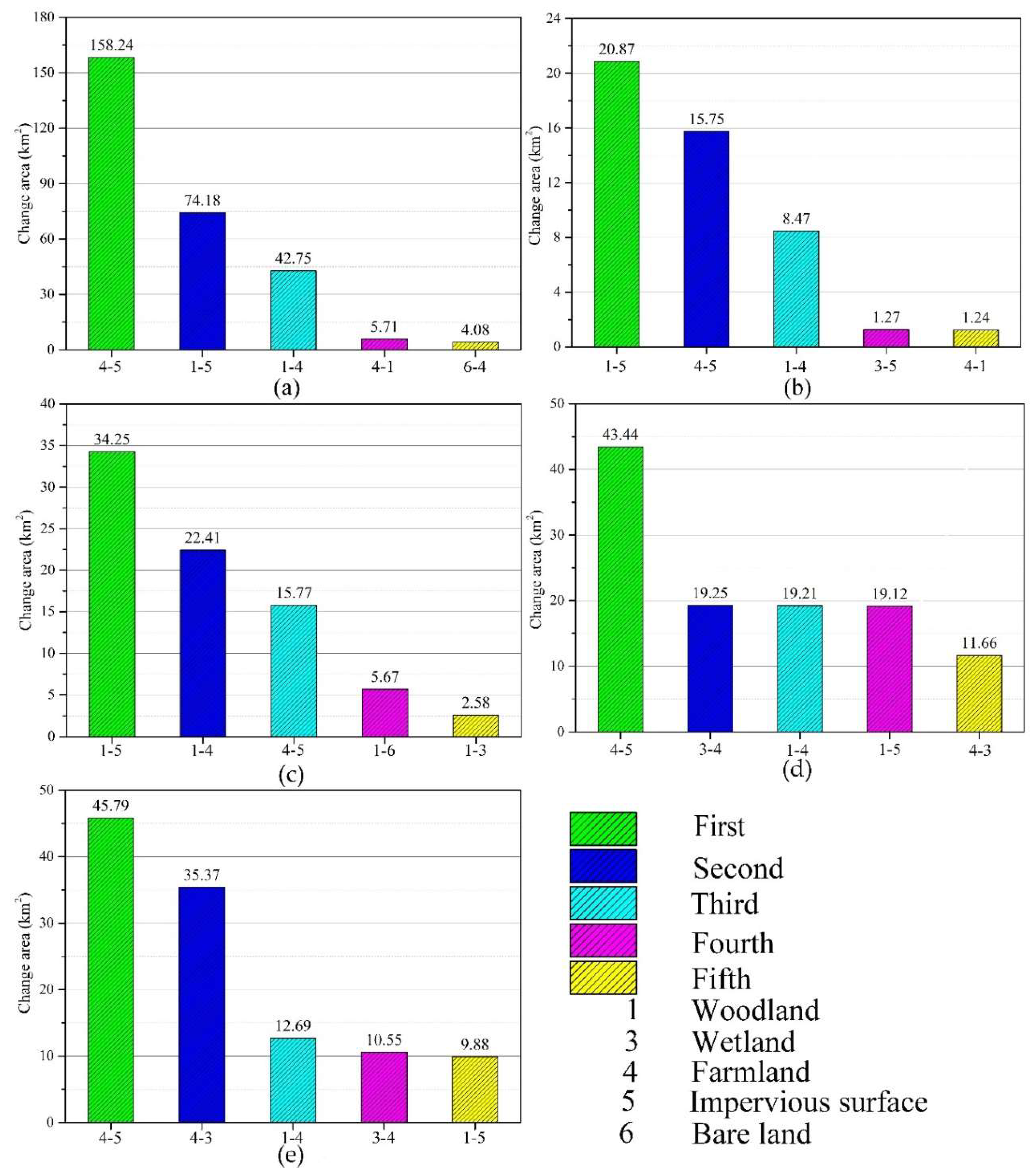
4.1.3. Spatial Pattern at Prefecture Level
5. Discussion
5.1. Issues for OBIA
5.2. Driving Force of Land Use Pattern
5.3. Driving Force of LUCC Pattern
5.4. Innovative Strategies
6. Conclusions
Supplementary Materials
Author Contributions
Funding
Acknowledgments
Conflicts of Interest
References
- Chen, Y.H.; Zhou, Y.N.; Ge, Y.; An, R.; Chen, Y. Enhancing Land Cover Mapping through Integration of Pixel-Based and Object-Based Classifications from Remotely Sensed Imagery. Remote Sens. 2018, 10, 77. [Google Scholar] [CrossRef]
- Engelen, G.; White, R. Validating and Calibrating Integrated Cellular Automata Based Models of Land Use Change. In The Dynamics of Complex Urban Systems; Albeverio, S., Andrey, D., Giordano, P., Vancheri, A., Eds.; Physica-Verlag HD: Heidelberg, Germany, 2008; pp. 185–211. [Google Scholar]
- Kok, J.L.D.; Overloop, S.; Engelen, G. Screening models for integrated environmental planning–A feasibility study for Flanders. Futures 2017, 88, 55–56. [Google Scholar] [CrossRef]
- Soleimani, A.; Hosseini, S.M.; Bavani, A.R.M.; Jafari, M.; Francaviglia, R. Simulating soil organic carbon stock as affected by land cover change and climate change, Hyrcanian forests (northern Iran). Sci. Total Environ. 2017, 599, 1646–1657. [Google Scholar] [CrossRef] [PubMed]
- White, R.; Uljee, I.; Engelen, G. Integrated modelling of population, employment and land-use change with a multiple activity-based variable grid cellular automaton. Int. J. Remote Sens. 2012, 26, 1256–1281. [Google Scholar] [CrossRef]
- Batty, M.; Marshall, S. The origins of complexity theory in cities and planning. In Complexity Theories of Cities Have Come of Age; Springer: Berlin/Heidelberg, Germany, 2012; pp. 21–45. [Google Scholar]
- Deng, X.Z.; Shi, Q.L.; Zhang, Q.; Shi, C.C.; Yin, F. Impacts of land use and land cover changes on surface energy and water balance in the Heihe River Basin of China, 2000–2010. Phys. Chem. Earth 2015, 79, 2–10. [Google Scholar] [CrossRef]
- Cockx, K.; Van de Voorde, T.; Canters, F.; Poelmans, L.; Uljee, I.; Engelen, G.; de Jong, K.; Karssenberg, D.; Kwast, J. Incorporating land-use mapping uncertainty in remote sensing based calibration of land-use change. In Proceedings of the 8th International Symposium on Spatial Data Quality, Hong Kong, China, 30 May–1 June 2013; Volume XL-2/W1, pp. 7–12. [Google Scholar]
- Jin, S.; Yang, L.; Zhu, Z.; Homer, C. A land cover change detection and classification protocol for updating Alaska NLCD 2001 to 2011. Remote Sens. Environ. 2017, 195, 44–55. [Google Scholar] [CrossRef]
- Hao, M.; Shi, W.Z.; Deng, K.H.; Zhang, H.; He, P.F. An object-based change detection approach using uncertainty analysis for VHR images. J. Sens. 2016, 2016, 1–17. [Google Scholar] [CrossRef]
- Chirici, G.; Mura, M.; Mcinerney, D.; Py, N.; Tomppo, E.O.; Waser, L.T.; Travaglini, D.; Mcroberts, R.E. A meta-analysis and review of the literature on the k-Nearest Neighbors technique for forestry applications that use remotely sensed data. Remote Sens. Environ. 2016, 176, 282–294. [Google Scholar] [CrossRef]
- Hussain, M.; Chen, D.; Cheng, A.; Wei, H.; Stanley, D. Change detection from remotely sensed images: From pixel-based to object-based approaches. ISPRS J. Photogramm. Remote Sens. 2013, 80, 91–106. [Google Scholar] [CrossRef]
- Baker, B.A.; Warner, T.A.; Conley, J.F.; McNeil, B.E. Does spatial resolution matter? A multi-scale comparison of object-based and pixel-based methods for detecting change associated with gas well drilling operations. Int. J. Remote Sens. 2013, 34, 1633–1651. [Google Scholar] [CrossRef]
- Sen, S.; Zipper, C.E.; Wynne, R.H.; Donovan, P.F. Identifying Revegetated mines as disturbance/recovery trajectories using an Interannual Landsat Chronosequence. Photogramm. Eng. Remote Sens. 2012, 78, 223–235. [Google Scholar] [CrossRef]
- Zhai, D.L.; Dong, J.W.; Cadisch, G.; Wang, M.C.; Kou, W.L.; Xu, J.C.; Xiao, X.M.; Abbas, S. Comparison of Pixel- and Object-Based Approaches in Phenology-Based Rubber Plantation Mapping in Fragmented Landscapes. Remote Sens. 2018, 10, 1–20. [Google Scholar] [CrossRef]
- Blaschke, T.; Hay, G.J.; Kelly, M.; Lang, S.; Hofmann, P.; Addink, E.; Feitosa, R.Q.; Meer, F.V.D.; Werff, H.V.D.; Coillie, F.V. Geographic Object-Based Image Analysis â—Towards a new paradigm. ISPRS J. Photogramm. Remote Sens. 2014, 87, 180–191. [Google Scholar] [CrossRef] [PubMed]
- Georganos, S.; Grippa, T.; Vanhuysse, S.; Lennert, M.; Shimoni, M.; Kalogirou, S.; Wolff, E. Less is more: Optimizing classification performance through feature selection in a very-high-resolution remote sensing object-based urban application. GISci. Remote Sens. 2018, 55, 221–242. [Google Scholar] [CrossRef]
- Ma, L.; Li, M.C.; Ma, X.X.; Cheng, L.; Du, P.J.; Liu, Y.X. A review of supervised object-based land-cover image classification. ISPRS J. Photogramm. Remote Sens. 2017, 130, 277–293. [Google Scholar] [CrossRef]
- Lu, L.; Tao, Y.; Di, L. Object-based plastic-mulched landcover extraction using integrated Sentinel-1 and Sentinel-2 data. Remote Sens. 2018, 10, 1820. [Google Scholar] [CrossRef]
- Nemmaoui, A.; Aguilar, M.; Aguilar, F.; Novelli, A.; Lorca, A. Greenhouse crop identification from multi-temporal multi-sensor satellite imagery using object-based approach: a case study from Almería (Spain). Remote Sens. 2018, 10, 1751. [Google Scholar] [CrossRef]
- Durieux, L.; Kropáček, J.; de Grandi, G.D.; Achard, F. Object-oriented and textural image classification of the Siberia GBFM radar mosaic combined with MERIS imagery for continental scale land cover mapping. Int. J. Remote Sens. 2007, 28, 4175–4182. [Google Scholar] [CrossRef]
- Toure, S.; Stow, D.; Shih, H.C.; Coulter, L.; Weeks, J.; Engstrom, R.; Sandborn, A. An object-based temporal inversion approach to urban land use change analysis. Remote Sens. Lett. 2016, 7, 503–512. [Google Scholar] [CrossRef]
- Geurs, K.; Hoen, A.; Engelen, G.; van Wee, B. 30 years of spatial planning and infrastructure policies in the Netherlands: A success? In Proceedings of the Bijdrage Colloquium Vervoersplanologisch Speurwerk, Antwerpen, Belgium, 20–21 November 2003; pp. 151–170. [Google Scholar]
- Su, M.; Jiang, R.; Li, R.R. Investigating Low-Carbon Agriculture: Case Study of China’s Henan Province. Sustainability 2017, 9, 2295. [Google Scholar] [CrossRef]
- Peng, J.D.; Liao, Y.F.; Jiang, Y.H.; Zhang, J.M.; Qi, X.R. Development of the homogenized monthly precipitation series during 1910–2014 and its changes in Hunan Province, China. J. Water Clim. Chang. 2017, 8, 791–801. [Google Scholar] [CrossRef]
- Bureau, C.S. Hunan Statistical Yearbook; China Statistics Press: Beijing, China, 2011.
- Huang, H.X.; Luo, Y.P.; Yin, F.R.; Yi, M.; Liao, X.Y.; Hu, S.L.; Xing, H.L. Analysis on the driving forces of compositions and pattern changes of ecosystem in Hunan Province. J. Hunan Univ. Sci. Technol. 2015, 30, 61–67. [Google Scholar]
- Wu, M.Q.; Zhang, X.Y.; Huang, W.J.; Niu, Z.; Wang, C.Y.; Li, W.; Hao, P.Y. Reconstruction of Daily 30 m Data from HJ CCD, GF-1 WFV, Landsat, and MODIS Data for Crop Monitoring. Remote Sens. 2015, 7, 16293–16314. [Google Scholar] [CrossRef]
- Bernstein, L.S.; Jin, X.M.; Gregor, B.; Adler-Golden, S.M. Quick atmospheric correction code: Algorithm description and recent upgrades. Opt. Eng. 2012, 51, 111719–111724. [Google Scholar] [CrossRef]
- Xian, G.; Homer, C.; Fry, J. Updating the 2001 National Land Cover Database land cover classification to 2006 by using Landsat imagery change detection methods. Remote Sens. Environ. 2009, 113, 1133–1147. [Google Scholar] [CrossRef]
- Zhao, Y.S. Principle and Method of Remote Sensing Application and Analysis; Science Press of China: Beijing, China, 2012. [Google Scholar]
- Liu, W.; Liu, J.; Kuang, W.; Jia, N. Examining the influence of the implementation of Major Function-oriented Zones on built-up area expansion in China. J. Geogr. Sci. 2017, 27, 643–660. [Google Scholar] [CrossRef]
- Dronova, I. Object-Based Image Analysis in Wetland Research: A Review. Remote Sens. 2015, 7, 6380–6413. [Google Scholar] [CrossRef]
- Drǎguţ, L.; Csillik, O.; Eisank, C.; Tiede, D. Automated parameterisation for multi-scale image segmentation on multiple layers. ISPRS J. Photogramm. 2014, 88, 119–127. [Google Scholar] [CrossRef]
- Schultz, B.; Immitzer, M.; Formaggio, A.; Sanches, I.; Luiz, A.; Atzberger, C. Self-guided segmentation and classification of multi-temporal Landsat 8 images for crop type mapping in southeastern Brazil. Remote Sens. 2015, 7, 14482–14508. [Google Scholar] [CrossRef]
- Luo, K.; Li, R.D.; Chang, B.R.; Qiu, J.; Yi, F.J. Rearch progress in choosing objected-oriented optimal segmentation scale. World Sci. Technol. Res. Dev. 2013, 35, 75–79. [Google Scholar]
- Woldesenbet, A. Land use land cover change detection by using remote sensing data in Akaki River Basin. J. Food Agric. Environ. 2016, 1, 153–176. [Google Scholar]
- You, J.; Zhang, H.Q.; Chen, Y.F. Based on the GF-4 satellite image for the east dongting lake wetland vegetation type monitoring ability. J. Anhui Agric. Sci. 2018, 3, 33–39. [Google Scholar]
- Gomes, E.; Banos, A.; Abrantes, P.; Rocha, J. Assessing the Effect of Spatial Proximity on Urban Growth. Sustainability 2018, 10, 1308. [Google Scholar] [CrossRef]
- Jiankang, Z.; Jinxing, Z.; Huaiqing, Z.; Depeng, Y.; Ming, C.; Xiaorong, Z. Analysis on the driving force of the Returning Farmland to Lake Project and its impacts on wetland of West Dongting Lake. For. Resour. Manag. 2010, 4, 69–73. [Google Scholar]
- Alzamili, H.; El-Mewafi, P.D.M.; Beshr, A.; Hadeal, M.; Ashraf, D.; Beshr, M. Monitoring urban growth and land use change detection with GIS and remote sensing techniques in Daqahlia governorate Egypt. Int. J. Sustain. Built Environ. 2015, 6, 117–124. [Google Scholar] [CrossRef]
- Tang, F.H.; Chen, L.L. The evolution of regional differences of Changzhutan Urban Agglomeration since the 1990. Geogr. Res. 2011, 30, 94–102. [Google Scholar] [CrossRef]
- Liao, L.; Qin, J. Ecologica security of wetland in Chang-Zhu-Tan urban agglomeration. J. GeoInf. Sci. 2016, 18, 1217–1226. [Google Scholar] [CrossRef]
- Mallupattu, P.K.; Reddy, J.R.S. Analysis of Land Use/Land Cover Changes Using Remote Sensing Data and GIS at an Urban Area, Tirupati, India. Sci. World J. 2013, 2013, 1–6. [Google Scholar] [CrossRef] [PubMed]


| Spectral Band | Spatial Resolution | Spectral Range |
|---|---|---|
| Band 1: blue | 30 m | 0.43–0.52 μm |
| Band 2: green | 30 m | 0.52–0.60 μm |
| Band 3: red | 30 m | 0.63–0.69 μm |
| Band 4: near infrared | 30 m | 0.76–0.90 μm |
| Land Cover | Index | Threshold | Note |
|---|---|---|---|
| Wetland | Band 4s | Band 4s ≤ 1350~1403 | Band 4s are the fourth band of HJ-CCD in summer |
| Non-wetland | Band 4s | Band 4s > 1350~1403 | Same as above |
| Vegetation | NDVIs | NDVIs ≥ 0.32~0.42 | NDVI is the NDVI value of HJ-CCD in summer |
| Non-vegetation | NDVIs | NDVIs ˂ 0.32~0.42 | Same as above |
| Farmland | SAVIs and slope | SAVIs ≤ 0.76~0.83 and Slope ≤ 22°~27° | SAVIs is the SAVI value of HJ-CCD in summer |
| Non-farmland | SAVIs and slope | SAVIs > 0.76~0.83 or Slope > 22°~27° | Same as above |
| Woodland | ACNDVI, DEM and texture (GCLM-A) | ACNDVI ≥ 1.38~1.43 and DEM ≥ 600 m and 0.21~0.31 ≤ GCLM-A ≤ 0.35~0.41 | ACNDVI is the sum of NDVI in spring, summer and winter, GCLM-A is gray-level co-occurrence matrix for all directions |
| Non-woodland (grassland) | ACNDVI, DEM and texture (GCLM-A) | ACNDVI < 1.38~1.43 or DEM< 600 m or GCLM-A < 0.21~0.31 or GCLM-A > 0.35~0.41 | Same as above |
| Impervious surface | Brightness and compactness | Brightness ≥ 960~1500 and compactness ≥ 0.27~0.32 | |
| Bare land | Brightness and compactness | Brightness ≥ 960~1500 or compactness ≥ 0.27~0.32 |
| Measured Data Type | Classification Data Type | Sum of Measured Data | ||||
|---|---|---|---|---|---|---|
| 1 | 2 | … | … | n | ||
| 1 | p11 | p21 | … | … | pn1 | p+1 |
| 2 | p12 | p22 | … | … | pn2 | p+2 |
| … | … | … | … | … | … | |
| … | … | … | … | … | … | |
| n | p1n | p2n | … | … | pnn | p+n |
| Sum of classification | p1+ | p2+ | … | … | pn+ | N |
| Land Cover | Woodland | Grassland | Wetland | Farmland | Impervious Surface | Bare Land | Transfer |
|---|---|---|---|---|---|---|---|
| Woodland | - | 15.62 | 18.19 | 200.98 | 214.39 | 22.20 | 471.38 |
| Grassland | 4.56 | - | 0.02 | 1.93 | 0.51 | 0.01 | 7.03 |
| Wetland | 34.94 | 1.47 | - | 66.76 | 24.58 | 4.37 | 132.12 |
| Farmland | 183.87 | 5.57 | 70.02 | - | 445.74 | 17.68 | 722.88 |
| Impervious surface | 1.28 | 0.08 | 1.55 | 6.62 | - | 0.04 | 9.57 |
| Bare land | 12.77 | 0.33 | 5.35 | 18.55 | 7.52 | - | 44.52 |
| Transferred into | 237.42 | 23.07 | 95.13 | 294.84 | 692.74 | 44.30 | - |
© 2018 by the authors. Licensee MDPI, Basel, Switzerland. This article is an open access article distributed under the terms and conditions of the Creative Commons Attribution (CC BY) license (http://creativecommons.org/licenses/by/4.0/).
Share and Cite
Luo, K.; Li, B.; Moiwo, J.P. Monitoring Land-Use/Land-Cover Changes at a Provincial Large Scale Using an Object-Oriented Technique and Medium-Resolution Remote-Sensing Images. Remote Sens. 2018, 10, 2012. https://doi.org/10.3390/rs10122012
Luo K, Li B, Moiwo JP. Monitoring Land-Use/Land-Cover Changes at a Provincial Large Scale Using an Object-Oriented Technique and Medium-Resolution Remote-Sensing Images. Remote Sensing. 2018; 10(12):2012. https://doi.org/10.3390/rs10122012
Chicago/Turabian StyleLuo, Kaisheng, Bingjuan Li, and Juana P. Moiwo. 2018. "Monitoring Land-Use/Land-Cover Changes at a Provincial Large Scale Using an Object-Oriented Technique and Medium-Resolution Remote-Sensing Images" Remote Sensing 10, no. 12: 2012. https://doi.org/10.3390/rs10122012
APA StyleLuo, K., Li, B., & Moiwo, J. P. (2018). Monitoring Land-Use/Land-Cover Changes at a Provincial Large Scale Using an Object-Oriented Technique and Medium-Resolution Remote-Sensing Images. Remote Sensing, 10(12), 2012. https://doi.org/10.3390/rs10122012