Seasonal Local Temperature Responses to Paddy Field Expansion from Rain-Fed Farmland in the Cold and Humid Sanjiang Plain of China

Abstract

Numerous studies have documented the effects of irrigation on local, regional, and global climate. However, most studies focused on the cooling effect of irrigated dryland in semiarid or arid regions. In our study, we focused on irrigated paddy fields in humid regions at mid to high latitudes and estimated the effects of paddy field expansion from rain-fed farmland on local temperatures based on remote sensing and observational data. Our results revealed much significant near-surface cooling in spring (May and June) rather than summer (July and August) and autumn (September), which was −2.03 K, −0.73 K and −1.08 K respectively. Non-radiative mechanisms dominated the local temperature response to paddy field expansion from rain-fed farmland in the Sanjiang Plain. The contributions from the changes to the combined effects of the non-radiative process were 123.6%, 95.5%, and 66.9% for spring (May and June), summer (July and August), and autumn (September), respectively. Due to the seasonal changes of the biogeophysical properties for rain-fed farmland and paddy fields during the growing season, the local surface temperature responses, as well as their contributions, showed great seasonal variability. Our results showed that the cooling effect was particularly obvious during the dry spring instead of the warm, wet summer, and indicated that more attention should be paid to the seasonal differences of these effects, especially in a region with a relatively humid climate and distinct seasonal variations.

1. Introduction

It has been widely documented that land use changes (LUC) play an important role in regulating local, regional, and global climate systems [1,2,3]. Numerous simulations and investigations have been performed on the effects of typical LUC, such as deforestation, afforestation, desertification, and urbanization, on regional climates [4,5,6,7]. LUC influence climate mainly through biogeochemical and biogeophysical processes [8]. The biogeochemical processes associated with changes in the carbon budget are usually performed at the global scale and require multi-decadal time series [9,10], while biogeophysical processes can influence the atmosphere through land surface energy balance at different time and spatial scales more directly [11,12,13]. The biogeophysical influences are mainly conducted through radiative properties, such as albedo, and non-radiative properties, such as evapotranspiration and roughness length [14]. With the aggravation of regional land development, biogeophysical processes have attracted increasing attention.

The biogeophysical effects of LUC on climate are mainly evaluated through climate models, remote sensing, and in situ measurements [15,16,17,18,19]. No matter which method was used, the physical mechanism should be explained by the energy budget and energy balance [3,9,20]. Taking tropical deforestation as an example, deforestation may exert a negative radiative forcing from the albedo increase; yet, a warming effect on the land surface was observed due to the reduced evapotranspiration and turbulent heat exchange [1,3,8]. Lee et al. proposed an energy redistribution factor that suggested the efficiency of vegetated ecosystems to dissipate energy from the surface through its inherent biogeophysical characteristics based on the energy balance equation, which can partition the local temperature responses to LUC into contributions from radiative and non-radiative processes [3]. This method can be used to study temperature responses from LUC, such as urban expansion and afforestation [11,21,22]. Especially, Bright et al. expanded this method to global scales based on remote sensing data, as well as the in situ observation data to detect the temperature responses and non-radiative process due to the land cover and land management changes [21].

Irrigation farmland has a significant potential to alter local climate through a lower surface albedo and higher evaporation and transpiration [23,24]. In contrast to rain-fed farmland, irrigation land with a smaller Bowen ratio can deplete large amounts of heat during evapotranspiration and can be regarded as cooling islands, like wetlands [23,25]. The magnitude of temperature cooling may be comparable to or even exceed the warming effect from greenhouse gas increases or urbanization in some regions [26,27,28]. Cook et al. investigated the importance of irrigation to climate based on a new set of historically forced global climate model (GCM) experiments and found that the cooling is regionally focused and is especially strong in western North America, the Mediterranean, the Middle East, and Asia [29]. Lobell et al. used the community atmosphere model (CAM) equipped with an irrigation fraction dataset to evaluate the effect of irrigation on temperatures in several major irrigated regions of the world, which indicated potentially large differences of the temperature responses in different irrigation regions, with some regions cooling by 10 °C and others showing little change [30]. As the first order impact of irrigation on surface temperature is localized, the regional climate model (RCM) coupled with different irrigation schemes were widely used to detect the characteristics [31,32,33,34]. Alter et al. found that the irrigation in the center of United States can lead to a cooling of 0.75–1 °C in July to August [31]. Huang and Paul found that the irrigation in California’s Central Valley cooled the daily maximum near-surface temperature (Tmax) by approximately 1.1 °C based on the community earth system model (CESM) [32]. Based on a dynamic irrigation scheme for weather research and forecasting model (WRF), Wu et al. found that the irrigation in North China can decrease the average spring and summer temperature by 0.8–1.6 °C and 1.2–2.6 °C, respectively [33].

Though numerous climate models have investigated and demonstrated the direct temperature cooling of irrigation [23,30,35,36,37], great uncertainties remain, especially for the daily minimum temperature [32]. Kanamaru and Kanamitsu proposed that irrigation increased the daily minimum temperature [38], while Huber et al. found that the irrigation decreased daily minimum temperature [39]. Furthermore, the magnitude of the cooling from the simulation can be different due to different models and irrigation schemes [33,40]. The irrigation method, such as drip, sprinkler, and flood, and the precision of irrigation dataset used in the irrigation scheme can definitely influence the range of the temperature responses [41]. As a new observation technology over continuous space, remote sensing supplied a novel approach to evaluate the surface temperature responses and its corresponding mechanisms caused by irrigation [42].

The Sanjiang Plain, located in Northeast China, has experienced a rapid conversion from rain-fed farmland to paddy fields from 2005 to 2015 to pursue high economic interests [43]. Paddy fields, a typical irrigation land, can directly influence the energy balance and local temperature [24]. However, the irrigation method of paddy fields is different from that shown in the previous studies, that the water in the paddy fields was kept at a certain level at the early of the growing periods and depleted gradually at the end of the growing periods. Therefore, it is still unclear how paddy field expansion affects the local temperature and what the impact mechanism is in radiative and non-radiative process distribution.

In this study, we focused on paddy field expansion from rain-fed farmland and its biogeophysical effects on the local surface temperature in the Sanjiang Plain. First, we compared surface albedo and vegetation evaporation between rain-fed farmland and paddy fields based on remote sensing data to quantify and understand their biogeophysical differences during the growing season. Then, the energy balance model proposed by Lee et al. [3] was used to estimate the energy redistributor factor and evaluate the land surface temperature changes caused by paddy field expansion. Finally, we discussed the uncertainties of land surface temperature responses for this multi-year study and compared our results with other studies. Overall, we quantified the temperature effects due to paddy field expansion from rain-fed farmland and the biogeophysical mechanism, which may be helpful for understanding and modeling climate change, both in the past and future, and can provide suggestions and valuable information for land use management and adjustment.

2. Materials and Methods

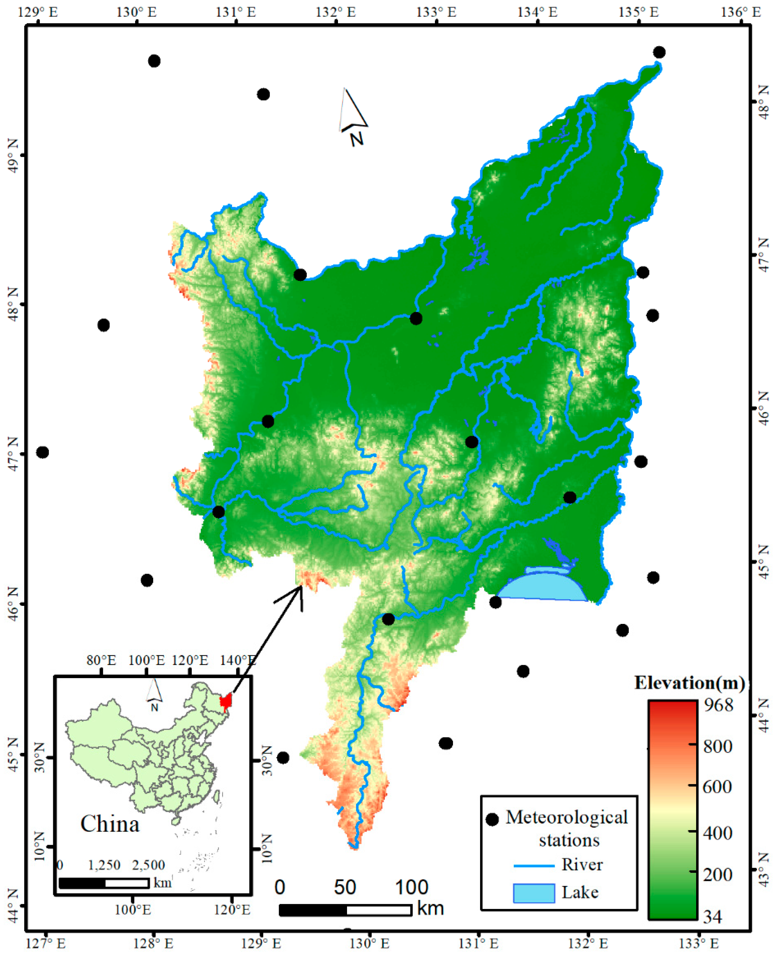
2.1. Study Area

The Sanjiang Plain is located in northeastern China and extends from 45°01′00″ N to 48°27′56″ N and 130°13′00″ E to 135°05′26″ E (see Figure 1). With a 108.9 thousand km² area, the Sanjiang Plain is an alluvial low plain with densely covered rivers. The typical geomorphic features of the Sanjiang Plain include broad alluvial low plains, terraces, and floodplains. The climate in the Sanjiang Plain is temperate humid or sub-humid continental monsoon climate [44]. The average annual precipitation and temperature are approximately 500–650 mm and 1–4 °C, respectively [45]. Winter here is long, dry, and cold, while summer is short, mild, and moist.

However, with large-scale agricultural development after the 1950s, a large area of wetlands was reclaimed into farmland [43]. The natural ecological environment, which was mainly composed of the original forest, grassland, and swamp, was transformed into an artificial ecological environment dominated by farmland, leading to severe land degradation and ecological environment deterioration [44,45,46,47,48]. However, since 2005, a large amount of rain-fed farmland has been converted to paddy fields to pursue higher economic benefits [49]. As a result, the crop type for the conversion areas has changed from corn to rice, which provides a good case for studying the climate effects caused by land use management.

2.2. Data Processing

Based on our previous studies, we developed the land use maps in 2005 and 2015 with human-computer interaction interpretation based on the Landsat 5 Thematic Mapper (TM) images in 2005 and Landsat 8 Operational Land Imager (OLI) images in 2015 (https://glovis.usgs.gov/) [43,49]. Only images in May and June were used in the classification to distinguish the paddy fields from rain-fed farmland. We used the land use classification system of China proposed by Liu in this study, which includes 6 first level classes and 25 subclasses [50]. The spatial resolution was 30 m and the overall accuracy of the 25 land use subclasses was 91.2% and the kappa index was 0.88 [49]. To illustrate the paddy field expansion process more clearly in the Sanjiang Plain, we used the five first level classes including forestland, grassland, waters, built-up, and marshes, and two subclasses including rain-fed farmland and paddy fields to conduct the LUC analysis (Figure 2). A 1-km fishnet was used to clip the land use data as well as the land use change maps derived from the land use maps in 2005 and 2015 to calculate the percentage of each land use type and the land use change percentage in each 1-km pixel. Considering the valid contrast between land use types as well as a sufficient number of sample grids, only a percentage of each land use type higher than 90% in each 1-km pixel were regarded as pure grids in the analysis, while we assume that the influence of other land use types that was less than 10% in each pixel would be randomly detrended. In addition, we used the spatial overlay analysis tool in ArcGIS (Environmental Systems Research Institute (Esri), Redlands, California, United States) to extract the unchanged pure land use pixels from 2005 to 2015. The number of unchanged paddy fields and rain-fed farmland pixels are 1202 and 5730 respectively. Only the unchanged pure rain-fed farmland and paddy fields were used for the comparison of biogeophysical characteristics such as albedo and evapotranspiration, as well as an energy redistribution factor in the following section.

We used the 16-day composite Moderate Resolution Imaging Spectroradiometer (MODIS) albedo product (MCD43B3.V005), which was closed in 2018, including the black and white sky albedo, to calculate the land surface albedo in our study area. Based on the diffuse skylight ratio deprived in our study area, we calculated the actual surface albedo [51]. The 8-day composite MODIS global evapotranspiration product (MOD16A2.V006), which is the most widely used evapotranspiration data, was used to obtain the vegetation evapotranspiration for each land cover type [52]. We also used the MODIS land surface temperature product (MYD11A2.V006) to obtain the land surface temperature (T_s in this paper) for our study area. The Aqua overpass time for our study area mainly ranged from 11:00 a.m. to 14:30 p.m. in the daytime and 23:00 p.m. to 2:30 a.m. during night, while the overpass time for Terra was earlier than that of Aqua (https://scool.larc.nasa.gov/en_rover_overpass.html). As the 8-day composite product is the synthesis of daily observation results, MYD11A2 data is more suitable than MOD11A2 in this study to represent daytime and nighttime surface temperature. We averaged the daytime and nighttime surface temperature to estimate the daily average surface temperature during the composite period.

We also used meteorological observation data, including the monthly air temperature at 2 m (Ta in this paper), and sunshine duration in situ data to obtain their spatial distributions in our study area based on ANUSPLIN software (Australia) and the Kriging interpolation method, respectively. The meteorological observation data were obtained from the China Meteorological Data Service Center (http://data.cma.cn/en) and Global Summary of the Day (GSOD) datasets from the National Climate Data Center (ftp://ftp.ncdc.noaa.gov/pub/data/gsod), both of which are the latest version after quality control. A total of 22 stations were included in the interpolation, in which 11 stations were from China while 11 stations were from the neighbor areas in Russia. As the air temperature was highly affected by elevation, we used the elevation information generated from ASTER DEM (advanced spaceborne thermal emission and reflection radiometer global digital elevation model) as the covariant to interpolate the spatial air temperatures, according to the spline interpolation method of ANUSPLIN [53]. In addition, we obtained the monthly downward longwave radiation data from a reanalysis dataset of MERRA-2 (Modern Era Retrospective Analysis for Research and Applications, Version 2), which has a spatial resolution of 0.5° × 2/3° (see Reference [54]).

All data, except the land use data used in the analysis, were 10-year averages from 2006 to 2015 to smooth the impact of random factors. In processing, we first calculated the composite time value for each variable and then aggregated the values to monthly means. Furthermore, we only selected good quality values of the MODIS product to calculate the albedo (mandator quality assessment = 0, indicating the best quality; or 1, indicating good quality), evapotranspiration (ET) (quality control = 0, indicating good quality) and land surface temperature (error flag = 0, indicating average land surface temperature (LST) error ≤1 K). The projection of all of the datasets used was transformed to Albers, and the spatial resolution was 1 km.

2.3. Methodology

2.3.1. Energy Redistribution Factor

Land surface temperature is greatly affected by the pattern of how the radiative energy is channeled into latent heat, and how sensible heat is dissipated away from the surface [3,21,55,56]. An expression of the energy redistribution factor was proposed as a combined measure of the aerodynamic and physiological controls governing surface energy budgets [3]. A higher value of the energy redistribution factor corresponds to a higher efficiency of non-radiative processes, either via evapotranspiration or the turbulent exchange of sensible heat, and is generally associated with lower temperature gradients at the surface–atmosphere boundary. For a certain land use type, based on the linearization of the surface longwave radiation term in the surface energy balance equation, the energy redistribution factor $f$ is introduced as [3]:

$$f=\frac{{\lambda }_0}{T_s-T_a}\left(R_n^{*}-G\right)-1$$

(1)

where ${\lambda }_0$ is the monthly mean Planck response to the external radiative forcing at the surface, which can be calculated as $1/4{\epsilon }_s\mathsf{\sigma }{T}_s^3$; ${\epsilon }_s$ is the surface emissivity, where we used a constant, 0.97, to approximate ${\epsilon }_s$ based on previous empirical findings [44,45]; σ is the Stefan–Boltzmann constant; T_s is the monthly mean land surface temperature (K); T_a is the monthly mean air temperature at 2 m (K). $R_n^{*}$ is the monthly mean apparent net radiation, and G is the monthly mean soil heat flux. Monthly mean apparent net radiation $R_n^{*}$ can be calculated using [21]:

$$R_n^{*}=S+L_{\downarrow }-\sigma T_a^4$$

(2)

where $S$ is the monthly net shortwave radiation flux, $L_{\downarrow }$ is the monthly downward longwave radiation flux. Monthly net shortwave radiation flux (S) and soil heat flux (G) are estimated using following empirical formulas respectively ([57], Equations (22), (24), and (28)):

$$S=\left(1-\alpha \right)\left(0.25+0.5\mathrm{r}\right)\times 37.586\mathrm{d}\left(\psi \sin \phi \sin \delta +\cos \phi \cos \delta \sin \psi \right)$$

(3)

$$G=0.14\left(T_{a,n}-T_{a,n-1}\right)$$

(4)

where $\alpha$ is the surface albedo, $\mathrm{r}$ is the percentage of sunshine, $\mathrm{d}$ is the relative distance from the Earth to the Sun, $\psi$ is the solar hour angle (rad), $\phi$ is the latitude (rad), and $\delta$ is the solar declination (rad). The factor $\left(0.25+0.5\mathrm{r}\right)37.586d\left(\psi \sin \phi \sin \delta +\cos \phi \cos \delta \sin \psi \right)$ represented the incoming solar radiation at the surface ($S_{\downarrow }$). n in Equation (4) is the time series of the month (1,2…12). Finally, the units of S and G are converted to W/m².

2.3.2. Surface Temperature Changes to LUC

Considering that local paddy fields and the surrounding rain-fed farmlands share the same background climate, the surface temperature response ($\Delta T_s$) to LUC, indicating surface temperature change due to land use change from rain-fed farmlands to paddy fields, is approximated using [21]:

$$\Delta T_s=\frac{{\lambda }_0}{\left(1+f\right)}\Delta S+\frac{-{\lambda }_0}{\left(1+f\right)}\Delta G+\frac{-{\lambda }_0}{{\left(1+f\right)}^2}\left(R_n^{*}-G\right)\Delta f$$

(5)

where ${\lambda }_0$, $f$, $R_n^{*}$, and G are variables of rain-fed farmlands before land use change, $\Delta S=-S_{\downarrow }\times \Delta \alpha$, where $\Delta \alpha$ is the monthly albedo change between between paddy fields and rain-fed farmlands; $\Delta G$ is the change in the monthly mean heat diffused into/out of the subsurface between paddy fields and rain-fed farmlands. Both $\Delta \alpha$ and $\Delta G$ in Equation (5) are calculated based on the regional statistical mean values of rain-fed farmland and paddy fields. $\Delta f$ is the change in the monthly mean energy redistribution factor, indicating the variation of $f$ between paddy fields and rain-fed farmlands. As the energy redistribution factor of the Sanjiang Plain we calculated is a ten-year average value, which involves both properties of rain-fed farmland and paddy fields in the paddy field expansion areas, we used the regional statistical mean value of unchanged rain-fed farmland and unchanged paddy field pixels to indicate the change of the energy redistribution factor for paddy field expansion. Then the first, second, and third right hand terms in Equation (5) represent the contribution of the land surface temperature response from the albedo change ($\Delta \alpha$), the change in heat conducted by the surface medium ($\Delta G$), and the change in energy redistribution factor ($\Delta f$), respectively [21].

2.3.3. Uncertainty Analysis

As discussed in the section above, we have got the spatial continuous f values for the Sanjiang Plain but we used a regional mean f value to conduct analysis just because the spatial f values in the paddy expansion areas include both the information of the rain-fed farmland and paddy field during the study period. However, there were spatial differences for f due to different geographic conditions, such as elevation, soil moisture, and so on [3], resulting in spatial variations in the local surface temperature responses. Therefore, we used the spatial continuous f values which involved the LUC information in the Sanjiang Plain to discuss the uncertainties of ΔT_s at the pixel level.

We first assumed that all of the conversions from rain-fed farmland to paddy fields started and ended in 2006. Then, the f value in the conversion regions represents the near-real f value for the paddy fields. Based on the $\Delta f$, we obtained from the regional statistics, we could easily obtain the spatial distribution of the f values for rain-fed farmland in the conversion areas. Then, combined with the paddy field expansion percentage maps, the ΔT_s caused by the conversion from rain-fed farmland to paddy fields was estimated at the pixel level in the Sanjiang Plain. As conversion could have happened at any time during 2005 to 2015, the derived spatial continuous f values in the conversion regions should be less than the real value of the paddy fields. As a result, the f value for the original rain-fed farmland before the conversion became smaller than their real values, contributing to the potential maximum ΔT_s. On the other hand, we also assumed that the conversion occurred in 2015; then, the f values we derived represent the near real f values for rain-fed farmland before the conversion, resulting in the minimum ΔT_s. Then the difference between potential maximum ΔT_s and potential minimum ΔT_s represents the spatial uncertainties of the surface temperature responses.

3. Results

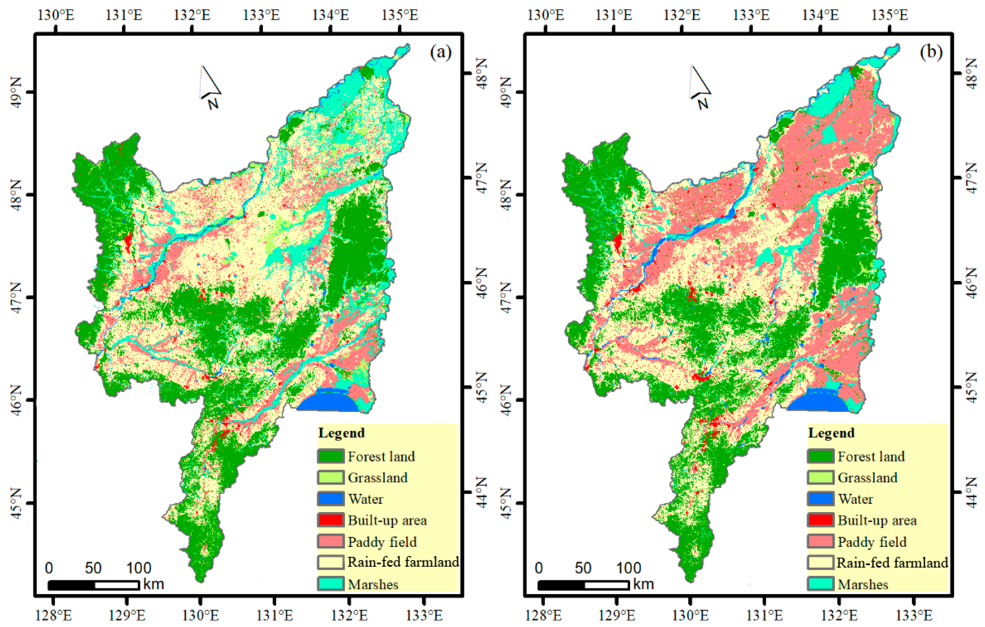
3.1. Paddy Field Expansion in the Sanjiang Plain

Figure 2 illustrates the spatial distribution of the main land use types of the Sanjiang Plain in 2005 and 2015. The four main land use types in 2005 were rain-fed farmland, forest land, paddy fields, and marshes, accounting for 37.4%, 30.7%, 12.1%, and 9.5% of the total area of the Sanjiang Plain, respectively. In 2015, the rain-fed farmland, forest land, and paddy fields became the dominant land use types, with an area proportion of 31.0%, 29.3%, and 26.2%, respectively. Based on the spatial comparison analysis between the two land use maps, we intuitively found that great land use changes took place in the Sanjiang Plain, among which the expansion of paddy fields was the most important and significant land use change during the ten years. Statistical analysis of the transfer matrix of land use shown in the supplement materials (Table S1) showed that more than 15% of the land of the Sanjiang Plain experienced paddy field expansion during 2005 to 2015, with 70% of the increase coming from conversion from rain-fed farmland, which is consistent with Yan’s study [43].

3.2. Comparison of Key Biogeophysical Parameters in Rain-Fed Farmland and Paddy Fields

LUC can strongly influence the biogeophysical characteristics of the land surface and lead to direct impacts on the surface energy balance and, in turn, on regional or local temperatures [1,2,9,18,58]. In our study, two biogeophysical parameters, albedo and evapotranspiration, which dominates radiative and non-radiative processes, respectively [19], were selected and analyzed for rain-fed farmland and paddy fields during the growing season. The convection change between rain-fed farmland and paddy fields was another important non-radiative process. The convection was affected by surface roughness, which could be obtained by crop height. This parameter change is not discussed here. Based on the 10-year-average monthly albedo and evapotranspiration data, the month-by-month changes of both parameters for unchanged pure pixels of rain-fed farmland and paddy fields were easily obtained. The mean and standard deviation of albedo and evapotranspiration characteristics for both rain-fed farmland and paddy fields were calculated using the 90th percentile range of unchanged land pixels, which were pixels above the 5th percentile and below the 95th percentile, to reducing the influence of singular values, the results of which are shown in Figure 3.

The regional statistic results showed that both rain-fed farmland and paddy fields had a similar change tendency for albedo and ET during the growing season. Generally, the albedo of water was lower than that of other land use types [59], and as a result, the albedo of paddy fields was much lower than that of rain-fed farmland in May and June when the paddy fields were filled with water. Significant albedo differences were detected in May and June (spring), −0.035 ± 0.031 and −0.028 ± 0.027, respectively. Due to the rapid increase of vegetation coverage in July and August (summer), the albedo mainly reflected the characteristics of crops instead of soil and became consistent between the two farmlands. The harvesting method of different crops, as well as the burning of straw in rain-fed farmland, may be the reason why the albedo in paddy fields was higher than that in rain-fed farmland in September. The Welch’s t-test showed that the difference in albedo between two different land cover types from May to September was statistically significant at a p < 0.05 significance level.

The ET for paddy fields showed a similar change trend during the growing season. The ET was very small at the beginning of the growing season. With the growing of crops, the ET increased rapidly from May and reached a maximum in July and August for paddy field lands and rain-fed farmland, respectively. In June and July, due to the adequate water under crops, the ET in paddy fields was significantly higher than that in rain-fed farmland, and the difference between the two farmlands reached 9.64 ± 17.78 mm and 12.29 ± 27.50 mm. Because of the water depletion of paddy fields and larger vegetation canopy of rain-fed land, the ET in rain-fed farmland exceeded that in the paddy fields by 8.44 ± 27.67 mm and 6.73 ± 13.64 mm in August and September, respectively. The ET differences between paddy fields and rain-fed farmland during the growing period were statistically significant at the significant level of 0.05.

From the above comparison, we observed that the difference of albedo and the ET between rain-fed farmland and paddy fields changed with the seasons. However, the sign of the differences changed from positive to negative or negative to positive from May to September, which was distinct to Kueppers’ study that the differences between irrigated land and natural vegetation didn’t reverse in the whole growing period [60]. The variable differences will increase the complexity and difficulty of simulating or analyzing the radiation balance and energy budget process, which can explain why the climate effect of rice paddies has a larger uncertainty in model simulations [24].

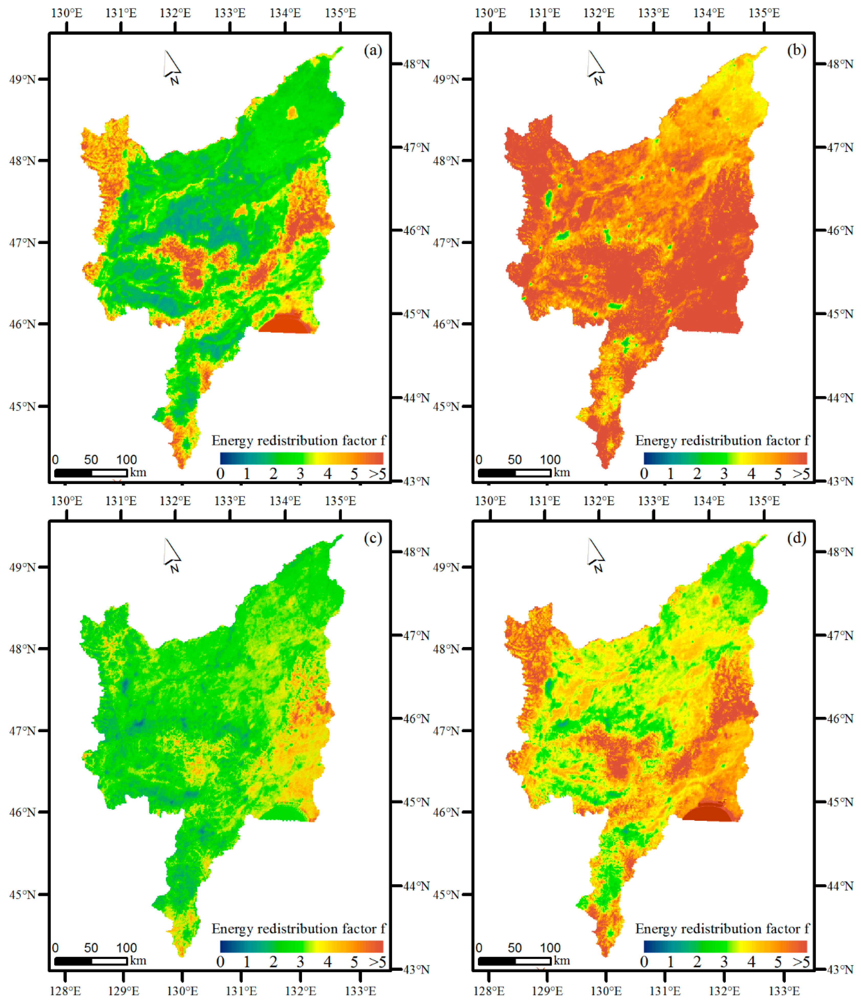
3.3. Energy Redistribution Factor f

There are obvious seasonal differences of biogeophysical parameters between rain-fed farmland and paddy fields, indicating seasonal differences in incoming solar radiation and energy exchanges as well as the energy redistribution factor f. Based on Equation (2), we obtained the spatial distribution of the energy redistribution factor f for spring (May and June), summer (July and August), autumn (September), and the growing season (May to September) (Figure 4).

The spatial continuous energy redistribution factor shown in Figure 4 can not only indicate the energy redistribution characteristic for special land use types but can also reflect the conversion information of LUC. For the unchanged land use pixels, the ten-year average f value at the pixel level represented the energy redistribution properties for each land use type, while for the changed land use pixels during 2005 to 2015, the ten-year average f value was the average of two or more land use types during the period. In general, the energy redistribution factor f of forests was highest among all land use types in the Sanjiang Plain, followed by marshes, paddy fields, rain-fed farmland, and urban land, which is consistent with previous results [21]. Interestingly, we also detected the seasonal variation of f for the Sanjiang Plain. At the regional scale, the annual mean difference of f between land use types may have covered up the strong seasonal signals to a certain extent, especially for crops that are mainly influenced by human beings. As shown in Figure 4, the f values in summer were higher than those in spring and autumn because the transpiration of vegetation reached its peak in summer and decreased in autumn. Through a spatial comparison between the land use maps and f values, we observed that the f values for paddy fields were higher than that for rain-fed farmland in spring and summer. More adequate soil moisture contributed to the greater capacity of shifting the Bowen ratio from sensible to latent heat flux in paddy fields [24].

In addition, we selected f values for the unchanged pure paddy fields and rain-fed farmland pixels from 2005 to 2015 to quantify the f values’ difference between the two farmlands. The Welch’s t-test showed that the difference in f between two different land cover types is statistically significant at p < 0.05 significance level. The inner 90 percentile values were used to calculate the mean f values for paddy fields and rain-fed farmland month-by-month (

Table 1. f values and Δf for unchanged pure pixels of paddy fields and rain-fed land during May to September, as well as the growing season in the Sanjiang Plain.

Land Type/Month	May	June	July	August	September	Growing Season
Paddy Fields	2.28	3.15	5.70	5.16	2.74	3.81
Rain-Fed Land	1.42	1.79	4.26	4.31	2.06	2.77
Δf	0.87	1.36	1.43	0.85	0.68	1.04

). Then the difference of f values (Δf) could be calculated through subtracting the f value of rain-fed farmland from that of paddy fields.

Overall, regardless of whether paddy fields or rain-fed farmland was considered, the f value increased first and then decreased from May to September. The peak value appeared in July when the f value of paddy fields was 5.70 and rain-fed farmland was 4.26. Δf showed a similar trend, with the highest values of 1.36 and 1.43 in June and July, respectively. Though the f values in August for rain-fed farmland and paddy fields were large, the Δf was only 0.85, which was lower than that in May because in late summer, vegetation transpiration, instead of both vegetation and soil evaporation, becomes the dominant factor influencing the latent heat transfer for both paddy fields and rain-fed farmland. The statistical results showed that in the growing season, the f values for paddy fields and rain-fed farmland were 3.81 ± 0.61 and 2.77 ± 0.48, respectively, resulting in a Δf of approximately 1.04.

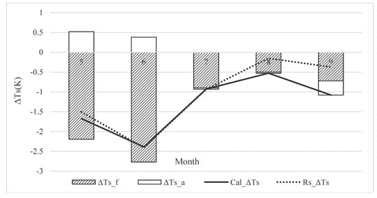
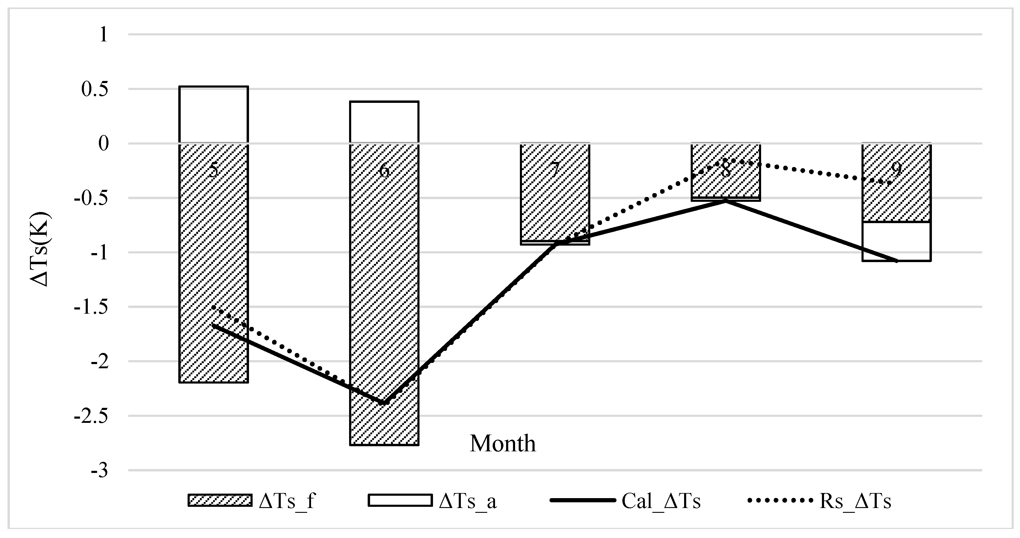
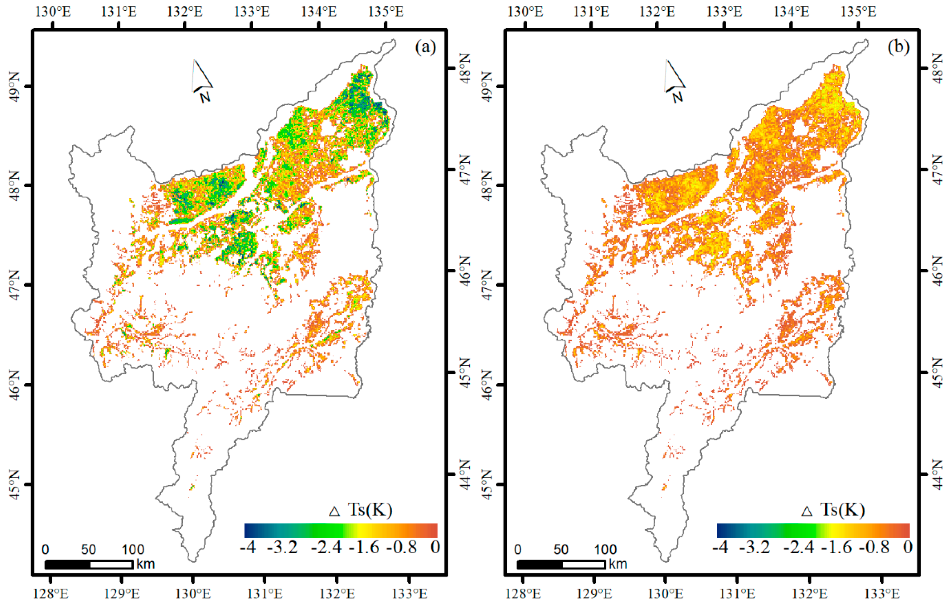
3.4. Land Surface Temperature Responses (ΔT_s) to Paddy Fields Expansion and Its Contributors

We used the regional statistical f values for rain-fed farmland shown in Table 1 to appropriate the real f values of the rain-fed farmland pixels in the Sanjiang plain before the paddy expansion. Then, based on the spatial 2006–2015 monthly mean climatologies of the net apparent heat flux, soil heat flux, air temperature, surface temperature, and surface albedo shown in Equation (5), we estimated the ΔT_s and its seasonal variation caused by paddy field expansion and its contribution components. It should be noted that only the change rate of the conversion from rain-fed farmland to paddy fields higher than 90% could be used as statistics.

The temperature responses to paddy field expansion and contributions from albedo changes (ΔT_s_a) and energy redistribution factor changes (ΔT_s_f) are shown in Figure 5. Consistent trends in temperature responses were not observed in spring through autumn. In general, conversion from rain-fed farmland to paddy fields led to a cooling effect within all months. It is interesting to note that the influence of f dominated the changes in land surface temperature rather than albedo. The contributions of f to ΔT_s were 123.6%, 95.5%, and 66.9% for spring (May and June), summer (July and August), and autumn (September), respectively, resulting in a 101.0% contribution during the growing season.

However, obvious seasonal differences for ΔT_s, as well as its contributions, were detected in the results. We found much significant near-surface cooling in spring (May and June) as opposed to summer (July and August) and autumn, which was −2.03 K, −0.73 K and −1.08 K, respectively. In spring (May and June), artificial irrigation allowed the paddy fields to have enough moisture for vegetation transpiration and water evaporation, which could remove a large amount of heat through latent heat flux and reduce the surface temperature by an average of 2.48 ± 0.17 K. In contrast to the effects of f, paddy field expansion led to a 0.45 ± 0.01 K warming effect through negative albedo changes. While in summer, although the soil moisture in the paddy fields was better than that of rain-fed farmland, the rapid growth of the vegetation canopy and humid climate led the gap of evapotranspiration and albedo between the two types of land to become smaller, especially in later summer, resulting in a smaller ΔT_s than that in spring. This result suggests that in summer on the Sanjiang Plain, soil moisture was not the main constraint factor for the evapotranspiration of different crops. In autumn, the albedo and evapotranspiration characteristic of paddy fields and rain-fed farmland became more similar as the water under vegetation has gradually evaporated or been absorbed by the crops, contributing to the lowest ΔT_s during the growing season. In addition to evapotranspiration, the ΔT_s_f included convection effects as well, which was another important non-radiative process. In summer and autumn, the crop height of paddy fields was less than that of rain-fed farmland. Therefore, the surface roughness and convection decreased for rain-fed farmland change to paddy fields, which resulted in a warming effect. The quantitative comparison of evapotranspiration cooling and convection warming should be further studied. In contrast to summer and spring, the albedo effect became negative as the albedo of paddy fields in autumn were higher than that of rain-fed farmland, as shown in Section 3.2.

We also compared the land surface temperature calculated based on Equation (5) with surface temperature obtained from MODIS data. The results showed that the Cal_ΔT_s was consistent with the Rs_ΔT_s for most months, indicating that the two contributors of the temperature responses including the albedo change (ΔT_s_a) and energy redistribution factor change (ΔT_s_f) could better reflect the radiative and non-radiative processes in regulating surface temperature.

Although the monthly daily mean surface temperature had significantly changed from rain-fed farmland to paddy fields, there were stronger daytime temperature decreases and nighttime temperature increases for paddy fields expansion from rain-fed farmland, especially in May and June. Based on MODIS data, we calculated that the daytime maximum surface temperature could decrease 5.98 K and 6.63 K from rain-fed farmland to paddy fields in May and June, respectively, while nighttime minimum surface temperature could increase 2.78 K and 2.40 K accordingly. The diurnal tendency for other months of the growing season was similar and less remarkable compared to May and June. It should be noted that the difference in LST of the growing season, for both daytime and nighttime between rain-fed farmland and paddy fields was statistically significant at a significance level of 0.05. The detailed information is shown in the supplement materials (Figure S1).

4. Discussion

4.1. The Uncertainties of ΔT_s at the Pixel Level

Based on the multi-year averaged and spatial continuous f values, other data mentioned in Section 2.3.2, as well as the two assumptions mentioned in Section 2.3.3, we calculated the potential maximum and minimum ΔT_s for the paddy expansion areas in the Sanjiang Plain. The results are shown in Figure 6.

Both Figure 6a,b showed significant spatial heterogeneity of the local surface temperature responses in the Sanjiang Plain. The stronger cooling effect corresponded to either the higher conversion ratio from rain-fed farmland to paddy fields or larger differences in the energy redistribution between paddy fields and rain-fed farmland according to the geophysical condition. Previous studies focusing on the effects from land use changes at the global scale showed that the local surface temperature responses varied across different geophysical environments [19,21], meaning that the geophysical conditions, such as soil moisture and temperature, may also be the reasons why the potential ΔT_s showed spatial differences. Furthermore, the difference between the potential maximum ΔT_s from Figure 6a and the potential minimum ΔT_s shown in Figure 6b represented the uncertainties of the land surface temperature response to paddy field expansion in the Sanjiang Plain. This also means that if we know the exact conversion time from rain-fed farmland to paddy filed in specific areas, we can deduce the real ΔT_s based on the potential maximum and minimum ΔT_s according to the degree of proximity to the two assumptions.

4.2. The Energy Redistribution Factor on the Local Scale

Compared with the energy redistribution factor for each land use type shown on the global scale [21], our spatial continuous f was estimated based on high-resolution remote sensing and meteorological observational datasets of surface properties, which allowed for a better representation of land surface heterogeneity and the energy budget between the land and atmosphere interface. Consistent with Bright’s study [21], our f values illustrated a similar ranking between land use types. In addition, our results also showed obvious seasonal variations of f values incorporating LUC information, which was essential to explain the seasonal temperature responses caused by LUC. With the intensification of human activities, the LUC was very significant in certain regions [38,61,62]. The pronouncedly LUC may bring difficulties in finding unchanged pure land use pixels to conduct the upscaling, resulting in no obvious climate signals caused by LUC in certain areas on the global scale [19,21]. In the Sanjiang Plain, the transformation from rain-fed farmland to paddy fields was both shown to be significant in our results and other studies [43]. Therefore, the energy redistribution factor derived from our results may be more suitable for evaluating the regional or local effects due to LUC.

4.3. Temperature Responses from Different Irrigation Types and Different Regions

The cooling effect signals of irrigation have been widely demonstrated across climate models and observations [23,24,25,26,27,28,29,30,63,64]. However, the magnitude of the effect varies according to differences in regional climate conditions as well as irrigation types [25,30,65,66]. Most studies have investigated the cooling effect caused by irrigation expansion from natural vegetation [23,25,27,31], while our study focused on temperature effects due to the conversion between two farmlands. Like Kueppers’ research [60], we found that the magnitude of the cooling effect had obvious seasonal variability. In his study, the largest temperature effects due to irrigation in the western United States were found in the dry summer months of July and August, while in our study, the temperature impacts of paddy field expansion were most pronounced in May and June, when the differences in soil moisture were the largest between paddy fields and rain-fed farmland. In the Sanjiang Plain, the paddy fields are the main irrigated agricultural land and require a large amount of irrigation in spring as opposed to the whole growing season [23]. In addition, the Sanjiang Plain has a humid climate condition, with rainfall mainly concentrated in July and August, resulting in the soil moisture not being the constraint factor to vegetation transpiration for rain-fed crops in summer. This is consistent with Lobell et al.’s study, which indicated little effect of irrigation in Northeast China compared with other irrigated areas over the world because of high soil moisture levels in northeast China [30]. Therefore, we can deduce that if the paddy field expansion occurred in semi-arid and arid areas, the cooling effect may become more significant and the largest temperature responses may occur in July or August instead of June or May. In other words, the cooling effect of irrigation is not only most pronounced during dry times of the year or during dry years [60] but may also be significant in dry regions.

On the other hand, the reason why the cooling effect was small in northeast China as shown in Lobell et al.’s study may be because the irrigation scheme used in their study was unified for all the major irrigated regions of the world [30]. Paddy fields irrigation is quite different from the dry farmland irrigation [24]. By comparing our results with those of previous studies, we found that there are great differences in the biogeophysical properties and temperature response mechanisms between irrigated paddy fields and irrigated dry land [24]. Paddy fields have lower albedos when there are standing water filled in spring than irrigated dryland, whose albedos are similar to those of deciduous broadleaf trees [60], resulting in a warmer radiative forcing. At the same time, paddy fields have a larger capacity to shift sensible heat to latent heat flux than irrigated dryland, which can contribute a greater cooling effect in spring as the non-radiative process dominates the temperature response across farmlands [15,21]. With the rapid growth of crops and depletion of the water in paddy fields in subsequent seasons, the cooling effect from irrigated dryland may exceed the paddy fields as irrigation continues in irrigated dryland. From another perspective, the crop types should be considered when we discuss the cooling effects caused by irrigation. Although Lu et al. incorporated the community land model 4 (CLM4) crop model into WRF3.3 to simulate the effects due to irrigation and showed a better description of the interaction between land and atmosphere, the irrigation schemes were not distinguished according to different crop types [40]. To better illustrate the energy and water balance of paddy fields through climate model, an irrigation scheme with a good representation of the hydrological dynamics should be developed.

4.4. Future Studies

In contrast to the temperature effects of wetland degradation during the 20th century [67], paddy field expansion led to a cooling effect during 2005 to 2015, which means that paddy expansion from rain-fed farmland has masked the warming signals caused by wetland degradation at the regional scale. However, though the paddy fields can be regarded as an artificial wetland, there are differences in its biogeophysical properties that regulate the water and energy budget [68,69]. From a long-term perspective, to what extent can the expansion of paddy fields alleviate the effect of wetland degradation and whether there is a seasonal feedback dislocation between the two land use changes are worthy of future study.

Furthermore, although the paddy fields in the Sanjiang Plain is likely to increase continually and induce a cooling effect in the future, the sustainability of the irrigation rates may be limited by the availability of groundwater resources [70]. If the groundwater resources become unsustainable, then the cooling effect may become the opposite and lead to food security issues [24]. Therefore, besides the energy balance, we should also pay attention to the water balance when simulating or analyzing the climate effects caused by paddy expansion.

5. Conclusions

In this study, the influence of paddy field expansion from rain-fed farmland on the local surface temperature as well as its radiative and non-radiative mechanisms was estimated in the Sanjiang Plain based on remote sensing and meteorological observation data. Our results revealed significant near-surface cooling in spring (May and June) rather than summer and autumn, which was −2.03 K, −0.73 K and −1.08 K, respectively, indicating that paddy expansion from rain-fed farmland may have masked the global warming signals in the Sanjiang Plain from 2005 to 2015. Consistent with Bright et al.’s study [15], non-radiative mechanisms dominated the local temperature response to paddy field expansion in the Sanjiang Plain. The contributions from the changes to the combined effects of the non-radiative process were 123.6%, 95.5%, and 66.9% for spring (May and June), summer (July and August), and autumn (September), respectively.

However, due to seasonal changes in the biogeophysical properties of rain-fed farmland and paddy fields during the growing seasons, ΔT_s, as well as its contributions, showed great seasonal variation. Our results showed that the cooling effect was significant, particularly during dry spring instead of warm, wet summer. This result indicates that we should pay more attention to the seasonal differences of the effects, especially in a region with a relatively humid climate and distinct seasonal variations. In addition, the uncertainties of spatial continuous ΔT_s were estimated based on two paddy expansion assumptions as well as the land use change percentage maps, indicating that we can obtain an appropriate pixel level ΔT_s if we know the exact conversion time and extent. Finally, our study provides a new case for studying the impacts of human-induced land use changes on the climate system, which can be as important as other land use changes, such as forest deforestation.

References

1. Feddema, J.J.; Oleson, K.W.; Bonan, G.B.; Mearns, L.O.; Buja, L.E.; Meehl, G.A.; Washington, W.M. The Importance of Land-Cover Change in Simulating Future Climates. Science 2005, 310, 1674–1678. [Google Scholar] [CrossRef] [PubMed]
2. Betts, R. Implications of Land Ecosystem-Atmosphere Interactions for Strategies for Climate Change Adaptation and Mitigation. Tellus Ser. B Chem. Phys. Meteorol. 2007, 59, 602–615. [Google Scholar] [CrossRef]
3. Lee, X.; Goulden, M.L.; Hollinger, D.Y.; Barr, A.; Black, T.A.; Bohrer, G.; Bracho, R.; Drake, B.; Goldstein, A.; Gu, L.H.; et al. Observed Increase in Local Cooling Effect of Deforestation at Higher Latitudes. Nature 2011, 479, 384–387. [Google Scholar] [CrossRef]
4. DeFries, R.S.; Bounoua, L.; Collatz, G.J. Human Modification of the Landscape and Surface Climate in the Next Fifty Years. Glob. Chang. Boil. 2002, 8, 438–458. [Google Scholar] [CrossRef]
5. Hanna, S.; Marciotto, E.; Britter, R. Urban Energy Fluxes in Built-up Downtown Areas and Variations across the Urban Area, for Use in Dispersion Models. J. Appl. Meteorol. Climatol. 2011, 50, 1341–1353. [Google Scholar] [CrossRef]
6. Yu, L.X.; Zhang, S.W.; Tang, J.M.; Liu, T.X.; Bu, K.; Yan, F.Q.; Yang, C.B.; Yang, J.C. The Effect of Deforestation on the Regional Temperature in Northeastern China. Theor. Appl. Climatol. 2015, 120, 761–771. [Google Scholar] [CrossRef]
7. Arnfield, A.J. Two Decades of Urban Climate Research: A Review of Turbulence, Exchanges of Energy and Water, and the Urban Heat Island. Int. J. Climatol. 2003, 23, 1–26. [Google Scholar] [CrossRef]
8. Davin, E.L.; de Noblet-Ducoudre, N. Climatic Impact of Global-Scale Deforestation: Radiative Versus Non-radiative Processes. J. Clim. 2010, 23, 97–112. [Google Scholar] [CrossRef]
9. Mahmood, R.; Pielke, R.A.; Hubbard, K.G.; Niyogi, D.; Dirmeyer, P.A.; McAlpine, C.; Carleton, A.M.; Hale, R.; Gameda, S.; Beltran-Przekurat, A.; et al. Land Cover Changes and Their Biogeophysical Effects on Climate. Int. J. Clim. 2014, 34, 929–953. [Google Scholar] [CrossRef]
10. Friedlingstein, P.; Dufresne, J.L.; Cox, P.M.; Rayner, P. How Positive Is the Feedback between Climate Change and the Carbon Cycle? Tellus Ser. B Chem. Phys. Meteorol. 2003, 55, 692–700. [Google Scholar] [CrossRef]
11. Chen, L.; Dirmeyer, P.A. Adapting Observationally Based Metrics of Biogeophysical Feedbacks from Land Cover/Land Use Change to Climate Modeling. Environ. Res. Lett. 2016, 11, 034002. [Google Scholar] [CrossRef]
12. Bonan, G.B. Forests and Climate Change: Forcings, Feedbacks, and the Climate Benefits of Forests. Science 2008, 320, 1444–1449. [Google Scholar] [CrossRef] [Green Version]
13. Winckler, J.; Reick, C.H.; Pongratz, J. Robust Identification of Local Biogeophysical Effects of Land-Cover Change in a Global Climate Model. J. Clim. 2017, 30, 1159–1176. [Google Scholar] [CrossRef]
14. Findell, K.L.; Shevliakova, E.; Milly, P.C.D.; Stouffer, R.J. Modeled Impact of Anthropogenic Land Cover Change on Climate. J. Clim. 2007, 20, 3621–3634. [Google Scholar] [CrossRef] [Green Version]
15. Bright, R.M. Metrics for Biogeophysical Climate Forcings from Land Use and Land Cover Changes and Their Inclusion in Life Cycle Assessment: A Critical Review. Environ. Sci. Technol. 2015, 49, 3291–3303. [Google Scholar] [CrossRef] [PubMed]
16. Pal, J.S.; Giorgi, F.; Bi, X.Q.; Elguindi, N.; Solmon, F.; Gao, X.J.; Rauscher, S.A.; Francisco, R.; Zakey, A.; Winter, J.; et al. Regional Climate Modeling for the Developing World—The Ictp RegCM3 and Regcnet. Bull. Am. Meteorol. Soc. 2007, 88, 1395–1410. [Google Scholar] [CrossRef]
17. Lawrence, P.J.; Chase, T.N. Investigating the Climate Impacts of Global Land Cover Change in the Community Climate System Model. Int. J. Climatol. 2010, 30, 2066–2087. [Google Scholar] [CrossRef]
18. Pielke, R.A.; Pitman, A.; Niyogi, D.; Mahmood, R.; McAlpine, C.; Hossain, F.; Goldewijk, K.K.; Nair, U.; Betts, R.; Fall, S.; et al. Land Use/Land Cover Changes and Climate: Modeling Analysis and Observational Evidence. Wiley Interdiscip. Rev. Clim. Chang. 2011, 2, 828–850. [Google Scholar] [CrossRef]
19. Li, Y.; Zhao, M.S.; Motesharrei, S.; Mu, Q.Z.; Kalnay, E.; Li, S.C. Local Cooling and Warming Effects of Forests Based on Satellite Observations. Nat. Commun. 2015, 6, 6603. [Google Scholar] [CrossRef] [PubMed]
20. Pielke, R.A.; Adegoke, J.O.; Chase, T.N.; Marshall, C.H.; Matsui, T.; Niyogi, D. A New Paradigm for Assessing the Role of Agriculture in the Climate System and in Climate Change. Agric. For. Meteorol. 2007, 142, 234–254. [Google Scholar] [CrossRef]
21. Bright, R.M.; Davin, E.; O’Halloran, T.; Pongratz, J.; Zhao, K.G.; Cescatti, A. Local Temperature Response to Land Cover and Management Change Driven by Non-Radiative Processes. Nat. Clim. Chang. 2017, 7, 296–303. [Google Scholar] [CrossRef]
22. Zhao, L.; Lee, X.; Smith, R.B.; Oleson, K. Strong Contributions of Local Background Climate to Urban Heat Islands. Nature 2014, 511, 216–219. [Google Scholar] [CrossRef] [PubMed]
23. Kueppers, L.M.; Snyder, M.A.; Sloan, L.C. Irrigation Cooling Effect: Regional Climate Forcing by Land-Use Change. Geophys. Res. Lett. 2007, 34. [Google Scholar] [CrossRef]
24. Puma, M.J.; Cook, B.I. Effects of Irrigation on Global Climate During the 20th Century. J. Geophys. Res. Atmos. 2010, 115. [Google Scholar] [CrossRef]
25. Sacks, W.J.; Cook, B.I.; Buenning, N.; Levis, S.; Helkowski, J.H. Effects of Global Irrigation on the near-Surface Climate. Clim. Dyn. 2009, 33, 159–175. [Google Scholar] [CrossRef]
26. Bonfils, C.; Lobell, D. Empirical Evidence for a Recent Slowdown in Irrigation-Induced Cooling. Proc. Natl. Acad. Sci. USA 2007, 104, 13582–13587. [Google Scholar] [CrossRef] [PubMed]
27. Lobell, D.B.; Bonfils, C.; Faures, J.M. The Role of Irrigation Expansion in Past and Future Temperature Trends. Earth Interact. 2008, 12, 1–11. [Google Scholar] [CrossRef]
28. Diffenbaugh, N.S. Influence of Modern Land Cover on the Climate of the United States. Clim. Dyn. 2009, 33, 945–958. [Google Scholar] [CrossRef]
29. Cook, B.I.; Shukla, S.P.; Puma, M.J.; Nazarenko, L.S. Irrigation as an Historical Climate Forcing. Clim. Dyn. 2015, 44, 1715–1730. [Google Scholar] [CrossRef]
30. Lobell, D.; Bala, G.; Mirin, A.; Phillips, T.; Maxwell, R.; Rotman, D. Regional Differences in the Influence of Irrigation on Climate. J. Clim. 2009, 22, 2248–2255. [Google Scholar] [CrossRef]
31. Alter, R.E.; Douglas, H.C.; Winter, J.M.; Eltahir, E.A.B. Twentieth Century Regional Climate Change During the Summer in the Central United States Attributed to Agricultural Intensification. Geophys. Res. Lett. 2018, 45, 1586–1594. [Google Scholar] [CrossRef]
32. Huang, X.Y.; Ullrich, P.A. Irrigation Impacts on California’s Climate with the Variable-Resolution CESM. J. Adv. Model. Earth Syst. 2016, 8, 1151–1163. [Google Scholar] [CrossRef]
33. Wu, L.Y.; Feng, J.M.; Miao, W.H. Simulating the Impacts of Irrigation and Dynamic Vegetation over the North China Plain on Regional Climate. J. Geophys. Res. Atmos. 2018, 123, 8017–8034. [Google Scholar] [CrossRef]
34. Aegerter, C.; Wang, J.; Ge, C.; Irmak, S.; Oglesby, R.; Wardlow, B.; Yang, H.S.; You, J.S.; Shulski, M. Mesoscale Modeling of the Meteorological Impacts of Irrigation During the 2012 Central Plains Drought. J. Appl. Meteorol. Climatol. 2017, 56, 1259–1283. [Google Scholar] [CrossRef]
35. Haddeland, I.; Lettenmaier, D.P.; Skaugen, T. Effects of Irrigation on the Water and Energy Balances of the Colorado and Mekong River Basins. J. Hydrol. 2006, 324, 210–223. [Google Scholar] [CrossRef]
36. Saeed, F.; Hagemann, S.; Jacob, D. Impact of Irrigation on the South Asian Summer Monsoon. Geophys. Res. Lett. 2009, 36. [Google Scholar] [CrossRef]
37. Douglas, E.M.; Beltran-Przekurat, A.; Niyogi, D.; Pielke, R.A.; Vorosmarty, C.J. The Impact of Agricultural Intensification and Irrigation on Land-Atmosphere Interactions and Indian Monsoon Precipitation—A Mesoscale Modeling Perspective. Glob. Planet. Chang. 2009, 67, 117–128. [Google Scholar] [CrossRef]
38. Kanamaru, H.; Kanamitsu, M. Model Diagnosis of Nighttime Minimum Temperature Warming During Summer Due to Irrigation in the California Central Valley. J. Hydrometeorol. 2008, 9, 1061–1072. [Google Scholar] [CrossRef]
39. Huber, D.; Mechem, D.; Brunsell, N. The effects of Great Plains irrigation on the surface energy balance, regional circulation, and precipitation. Climate 2014, 2, 103–128. [Google Scholar] [CrossRef]
40. Lu, Y.Q.; Harding, K.; Kueppers, L. Irrigation Effects on Land-Atmosphere Coupling Strength in the United States. J. Clim. 2017, 30, 3671–3685. [Google Scholar] [CrossRef]
41. Lawston, P.M.; Santanello, J.A.; Zaitchik, B.F.; Rodell, M. Impact of Irrigation Methods on Land Surface Model Spinup and Initialization of WRF Forecasts. J. Hydrometeorol. 2015, 16, 1135–1154. [Google Scholar] [CrossRef]
42. Zhou, D.C.; Li, D.; Sun, G.; Zhang, L.X.; Liu, Y.Q.; Hao, L. Contrasting Effects of Urbanization and Agriculture on Surface Temperature in Eastern China. J. Geophys. Res. Atmos. 2016, 121, 9597–9606. [Google Scholar] [CrossRef]
43. Yan, F.Q.; Zhang, S.W.; Liu, X.T.; Yu, L.X.; Chen, D.; Yang, J.C.; Yang, C.B.; Bu, K.; Chang, L.P. Monitoring Spatiotemporal Changes of Marshes in the Sanjiang Plain, China. Ecol. Eng. 2017, 104, 184–194. [Google Scholar] [CrossRef]
44. Song, K.S.; Wang, Z.M.; Du, J.; Liu, L.; Zeng, L.H.; Ren, C.Y. Wetland Degradation: Its Driving Forces and Environmental Impacts in the Sanjiang Plain, China. Environ. Manag. 2014, 54, 255–271. [Google Scholar] [CrossRef]
45. Wang, Z.M.; Zhang, B.; Zhang, S.Q.; Li, X.Y.; Liu, D.W.; Song, K.S.; Li, J.P.; Li, F.; Duan, H.T. Changes of Land Use and of Ecosystem Service Values in Sanjiang Plain, Northeast China. Environ. Monit. Assess. 2006, 112, 69–91. [Google Scholar] [CrossRef]
46. Zhang, S.W.; Zhang, Y.Z.; Li, Y.; Chang, L.P. Temporal and Spatial Characteristics of Land Use/Cover in Northeast China; Science Press: Beijing, China, 2006. [Google Scholar]
47. Zhang, J.Y.; Ma, K.M.; Fu, B.J. Wetland Loss under the Impact of Agricultural Development in the Sanjiang Plain, Ne China. Environ. Monit. Assess. 2010, 166, 139–148. [Google Scholar] [CrossRef]
48. Yan, F.Q.; Zhang, S.W.; Liu, X.T.; Chen, D.; Chen, J.; Bu, K.; Yang, J.C.; Chang, L.P. The Effects of Spatiotemporal Changes in Land Degradation on Ecosystem Services Values in Sanjiang Plain, China. Remote Sens. 2016, 8, 917. [Google Scholar] [CrossRef]
49. Yan, F.Q.; Yu, L.X.; Yang, C.B.; Zhang, S.W. Paddy Field Expansion and Aggregation since the Mid-1950s in a Cold Region and Its Possible Causes. Remote Sens. 2018, 10, 384. [Google Scholar] [CrossRef]
50. Liu, J.Y.; Liu, M.L.; Deng, X.Z. The Land Use and Land Cover Change Database and Its Relative Studies in China. J. Geogr. Sci. 2002, 12, 275–282. [Google Scholar]
51. Wang, C.Y.; Yang, J.C.; Myint, S.W.; Wang, Z.H.; Tong, B. Empirical Modeling and Spatio-Temporal Patterns of Urban Evapotranspiration for the Phoenix Metropolitan Area, Arizona. GIsci. Remote Sens. 2016, 53, 778–792. [Google Scholar] [CrossRef]
52. Mu, Q.Z.; Zhao, M.S.; Running, S.W. Improvements to a Modis Global Terrestrial Evapotranspiration Algorithm. Remote Sens. Environ. 2011, 115, 1781–1800. [Google Scholar] [CrossRef]
53. Yu, L.X.; Liu, T.X.; Cai, H.Y.; Tang, J.M.; Bu, K.; Yan, F.Q.; Yang, C.B.; Yang, J.C.; Zhang, S.W. Estimating Land Surface Radiation Balance Using Modis in Northeastern China. J. Appl. Remote Sens. 2014, 8, 083523. [Google Scholar] [CrossRef]
54. Gelaro, R.; Mccarty, W.; Suárez, M.J.; Todling, R.; Molod, A.; Takacs, L.; Randles, C.; Darmenov, A.; Bosilovich, M.; Reichle, R. The Modern-Era Retrospective Analysis for Research and Applications, Version 2 (MERRA-2). J. Clim. 2017, 30, 5419–5454. [Google Scholar] [CrossRef]
55. Juang, J.Y.; Katul, G.; Siqueira, M.; Stoy, P.; Novick, K. Separating the Effects of Albedo from Eco-Physiological Changes on Surface Temperature along a Successional Chronosequence in the Southeastern United States. Geophys. Res. Lett. 2007, 34. [Google Scholar] [CrossRef]
56. Vanden Broucke, S.; Luyssaert, S.; Davin, E.L.; Janssens, I.; van Lipzig, N. New Insights in the Capability of Climate Models to Simulate the Impact of Luc Based on Temperature Decomposition of Paired Site Observations. J. Geophys. Res. Atmos. 2015, 120, 5417–5436. [Google Scholar] [CrossRef]
57. Fischer, G.; Nachtergaele, F.O.; Prieler, S.; Teixeira, E.; Toth, G.; van Velthuizen, H.T.; Verelst, L.; Wiberg, D. Global Agro-Ecological Zones (GAEZ v3.0); IIASA: Laxenburg, Austria; FAO: Rome, Italy, 2012. [Google Scholar]
58. Pielke, R.A.; Marland, G.; Betts, R.A.; Chase, T.N.; Eastman, J.L.; Niles, J.O.; Niyogi, D.D.S.; Running, S.W. The Influence of Land-Use Change and Landscape Dynamics on the Climate System: Relevance to Climate-Change Policy Beyond the Radiative Effect of Greenhouse Gases. Philos. Trans. Math. Phys. Eng. Sci. 2002, 360, 1705–1719. [Google Scholar] [CrossRef] [PubMed]
59. Yu, L.X.; Liu, T.X.; Bu, K.; Yang, J.C.; Chang, L.P.; Zhang, S.W. Influence of Snow Cover Changes on Surface Radiation and Heat Balance Based on the WRF Model. Theor. Appl. Climatol. 2017, 130, 205–215. [Google Scholar] [CrossRef]
60. Kueppers, L.M.; Snyder, M.A.; Sloan, L.C.; Cayan, D.; Jin, J.; Kanamaru, H.; Kanamitsu, M.; Miller, N.L.; Tyree, M.; Due, H.; et al. Seasonal Temperature Responses to Land-Use Change in the Western United States. Glob. Planet. Chang. 2008, 60, 250–264. [Google Scholar] [CrossRef]
61. Fan, X.G.; Ma, Z.G.; Yang, Q.; Han, Y.H.; Mahmood, R.; Zheng, Z.Y. Land Use/Land Cover Changes and Regional Climate over the Loess Plateau During 2001–2009. Part I: Observational Evidence. Clim. Chang. 2015, 129, 427–440. [Google Scholar] [CrossRef]
62. Himiyama, Y. Land-Use Change and Regional Development in Hokkaido. In Land Use Changes in Comparative Perspective; Himiyama, Y., Hwang, M., Ichinose, T., Eds.; Science Publishers, Inc.: Plymouth, UK, 2002. [Google Scholar]
63. Ramankutty, N.; Foley, J.A. Estimating Historical Changes in Global Land Cover: Croplands from 1700 to 1992. Glob. Biogeochem. Cycles 1999, 13, 997–1027. [Google Scholar] [CrossRef]
64. Zhang, X.Z.; Xiong, Z.; Tang, Q.H. Modeled Effects of Irrigation on Surface Climate in the Heihe River Basin, Northwest China. J. Geophys. Res. Atmos. 2017, 122, 7881–7895. [Google Scholar] [CrossRef]
65. Selman, C.; Misra, V. The Impact of an Extreme Case of Irrigation on the Southeastern United States Climate. Clim. Dyn. 2017, 48, 1309–1327. [Google Scholar] [CrossRef]
66. Sorooshian, S.; Li, J.L.; Hsu, K.L.; Gao, X.G. How Significant Is the Impact of Irrigation on the Local Hydroclimate in California’s Central Valley? Comparison of Model Results with Ground and Remote-Sensing Data. J. Geophys. Res. Atmos. 2011, 116. [Google Scholar] [CrossRef]
67. Liu, Y.; Sheng, L.X.; Liu, J.P. Impact of Wetland Change on Local Climate in Semi-Arid Zone of Northeast China. Chin. Geogr. Sci. 2015, 25, 309–320. [Google Scholar] [CrossRef]
68. Natuhara, Y. Ecosystem Services by Paddy Fields as Substitutes of Natural Wetlands in Japan. Ecol. Eng. 2013, 56, 97–106. [Google Scholar] [CrossRef]
69. Zhou, Y.T.; Xiao, X.M.; Qin, Y.W.; Dong, J.W.; Zhang, G.L.; Kou, W.L.; Jin, C.; Wang, J.; Li, X.P. Mapping Paddy Rice Planting Area in Rice-Wetland Coexistent Areas through Analysis of Landsat 8 Oli and Modis Images. Int. J. Appl. Earth Obs. Geoinf. 2016, 46, 1–12. [Google Scholar] [CrossRef] [PubMed]
70. Kundzewicz, Z.W.; Doll, P. Will Groundwater Ease Freshwater Stress under Climate Change? Hydrol. Sci. J. 2009, 54, 665–675. [Google Scholar] [CrossRef]
Figure 1. Location and geographical features of the Sanjiang Plain.
Remotesensing 10 02009 g001
Figure 2. Land use maps of Sanjiang Plain in 2005 (a) and 2015 (b).
Remotesensing 10 02009 g002
Figure 3. Multi-year (2006–2015) mean albedo and evapotranspiration (ET) for unchanged pure pixels in rain-fed farmland and paddy fields during the growing season.
Remotesensing 10 02009 g003
Figure 4. Spatial distribution of the energy redistribution factor f in spring (a) (May and June), summer (b) (July and August), autumn (c) (September), and the growing season (d) (May to September) in the Sanjiang Plain. The growing season is from May to September, which was divided into three seasons according to the characters of Figure 3. The f values for the whole Sanjiang Plain was estimated based on 2006–2015 monthly mean climatologies of the net apparent heat flux, soil heat flux, air temperature, surface temperature, and surface albedo in each 1 km × 1 km pixel.
Remotesensing 10 02009 g004
Figure 5. Land surface temperature based on MODIS data (Rs_ΔTs) and Equation (5) (Cal_ΔTs), and contribution from albedo change (ΔTs_a) and energy redistribution factor change (ΔTs_f), responding to the conversion from rain-fed farmland to paddy fields.
Remotesensing 10 02009 g005
Figure 6. The uncertainties of ΔTs at pixel scale in the Sanjiang Plain. (a) The potential maximum ΔTs when we assumed all the paddy field expansion from rain-fed farmland occurred in 2006, and (b) the potential minimum ΔTs when we assumed the expansion occurred in 2015.
Remotesensing 10 02009 g006