Retrieval of Daily PM_2.5 Concentrations Using Nonlinear Methods: A Case Study of the Beijing–Tianjin–Hebei Region, China

Abstract

Exposure to fine particulate matter (PM_2.5) is associated with adverse health impacts on the population. Satellite observations and machine learning algorithms have been applied to improve the accuracy of the prediction of PM_2.5 concentrations. In this study, we developed a PM_2.5 retrieval approach using machine-learning methods, based on aerosol products from the Moderate Resolution Imaging Spectroradiometer (MODIS) aboard the NASA Earth Observation System (EOS) Terra and Aqua polar-orbiting satellites, near-ground meteorological variables from the NASA Goddard Earth Observing System (GEOS), and ground-based PM_2.5 observation data. Four models, which are orthogonal regression (OR), regression tree (Rpart), random forests (RF), and support vector machine (SVM), were tested and compared in the Beijing–Tianjin–Hebei (BTH) region of China in 2015. Aerosol products derived from the Terra and Aqua satellite sensors were also compared. The 10-repeat 5-fold cross-validation (10 × 5 CV) method was subsequently used to evaluate the performance of the different aerosol products and the four models. The results show that the performance of the Aqua dataset was better than that of the Terra dataset, and that the RF algorithm has the best predictive performance (Terra: R = 0.77, RMSE = 43.51 μg/m³; Aqua: R = 0.85, RMSE = 33.90 μg/m³). This study shows promise for predicting the spatiotemporal distribution of PM_2.5 using the RF model and Aqua aerosol product with the assistance of PM_2.5 site data.

1. Introduction

Recently, severe haze pollution over China, especially Eastern China, has received extensive attention. Fine particulate matter (PM_2.5: small inhalable solid and liquid particles suspended in the air with aerodynamic diameters of not more than 2.5 μm) consists mainly of ash haze that sharply influences the environment and air quality, as well as public health [1,2]. Though stationary ground measurements of PM_2.5 are routinely performed with high accuracy and sampling frequency, the measurements are limited by sporadic and uneven spatial coverage, as well as having point-based monitoring and excessively high construction costs. However, the retrieval of ground-level PM_2.5 concentrations from satellite remote sensors has become a good complementary technique for pollution monitoring, source tracking, the assessment of health effects, epidemiological studies, and the estimation of exposure and climate change [3,4].

The main satellite-derived parameter relevant to the estimation of surface PM_2.5 concentrations is the aerosol optical depth (AOD), which is defined as the integrated extinction coefficient by atmospheric particles from the Earth’s surface to the top of the atmosphere [5], while meteorological variables (e.g., planetary boundary layer height, wind speed, relative humidity, temperature, and atmospheric pressure) and other auxiliary datasets are also considered and tentatively incorporated as covariates to further enhance the estimation accuracy. Many satellite sensors have been launched and have provided reliable AOD retrievals (MISR, SeaWIFS, VIIRS, OMI, and GOES) [6,7,8,9,10]. The Moderate Resolution Imaging Spectroradiometer (MODIS) sensors, aboard the NASA Earth Observation System (EOS) Terra and Aqua polar-orbiting satellites, provide aerosol-related data, and are being acknowledged and used in many studies, due to their relatively mature aerosol retrieval algorithms and recalibration [11].

Methods utilizing satellite-based aerosol products to retrieve surface PM_2.5 concentrations are generally divided into three categories: global chemical transport model-based scaling factor methods [12,13,14], physical mechanism-based semiempirical formula methods [15,16,17], and empirical statistical models. The lack of emissions inventory data and the complexity of the physical mechanism of PM mass hamper the use of the former methods, and statistical models, especially advanced statistical models with high accuracy and wide applicability, are considered to be a compromise [18]. Regarding statistical methods, ordinary linear regression (LR) and multiple linear regression (MLR) models have been first and extensively adopted to reveal the relationship between the PM_2.5 mass concentration and satellite-derived AOD, and reasonable correlations of the modeled and observed PM_2.5 laid a solid foundation for the use of image AOD parameters [19]. Additionally, more complex nonlinear regression models, such as linear mixed effects models (LME), mixed-effects regression models [20], generalized linear models (GLM) [21], generalized additive models (GAM) [10,22], geographically weighted regression models (GWR) [23,24,25,26], and geographically and temporally weighted regression models (GTWR) [27] have also been applied and proven to enhance the capability of inferring PM_2.5 mass. Furthermore, some robust approaches have been formed recently by integrating two or several regression techniques to hierarchically estimate the surface PM_2.5 concentration, typically integrating LME with GWR models [28] and combining GAM with natural cubic splines (NS) [29], as well as building three-stage statistical models [30]. These approaches provide great improvements in model precision for the estimation of PM_2.5 concentration.

Interestingly, popular machine learning methods such as artificial neural network (ANN) [31], Bayesian maximum entropy (BME) [22], support vector regression (SVM) [32], and multivariate adaptive regression splines (MARS) [33], all yield more satisfactory performances compared with conventional statistical models, which exhibit the visible potential for the estimation of surface PM_2.5 concentration. Random forest (RF) models have several appealing properties and have emerged as a promising machine learning approach. RF has been used for PM_2.5 pollutant forecasting, air quality prediction, and historical monthly PM_2.5 concentration estimation, which has produced exciting results [34,35]. Considering that this potentially attractive technique has been successfully applied in many scientific disciplines despite still being in its infancy in remote-sensed daily PM_2.5 estimation problems, there is a relatively insufficient amount of studies comparing the predictions of these effective methods concerning PM_2.5 inversion research.

In this study, we aim to investigate and compare the performance of the current most advanced and efficient methods, RF and SVM, for the estimation of daily PM_2.5 concentration. At the same time, orthogonal regression (OR) [36] and regression tree (Rpart) [37] methods are also used as contrasting approaches. The ground-based PM_2.5 observations, meteorological parameters from the Goddard Earth Observing System (GEOS), and the Collection 6 fusion of dark target (DT) and deep blue algorithm (DB) aerosol products from the MODIS sensors on both the Terra and Aqua satellites for the year of 2015 over the Beijing–Tianjin–Hebei (BTH) region of China were used, and the 10-repeat 5-fold cross-validation method was used to evaluate all model accuracies. We also further verified the PM_2.5-inferring performance from the spatial and temporal distributions by mapping the PM_2.5 concentration distribution using the best-performing models and kriging interpolation of the parameters quantified at the sites.

2. Materials and Methods

2.1. Data Description

2.1.1. Ground Measurements

The BTH region lies in the northern part of the North China Plain, and one of the most economically vibrant metropolitan regions is located along Bohai Bay, extending from 113–120°E and 36–43°N (Figure 1). Updated hourly ground-based PM_2.5 measurements in this region are primarily obtained from the China Environmental Monitoring Center (CEMC), published through the “National Urban Air Quality Real-Time Publishing Platform” (http://113.108.142.147:20035/emcpublish/). In total, 79 new monitoring sites have been added to our study domain. Figure 1 demonstrates the elevation data (obtained from the Global Multi-Resolution Terrain Elevation Data, 2010) and the distribution of PM_2.5 monitoring stations (upper-right).

2.1.2. Satellite Data

The MODIS sensors aboard the EOS Terra and Aqua polar-orbiting satellites were launched in 1999 and 2002, respectively (see: https://modis.gsfc.nasa.gov/about/), and they observe the Earth at approximately 10:30 AM and 1:30 PM local time, with a broad swath of approximately 2330 km. The sensors possess a wide spectral range and high spatial coverage, and they make near-daily measurements. These measurements yield multiple datasets of aerosol optical depth for near-real-time monitoring, and a variety of other applications. The Collection 6 datasets have been proven to substantially increase the precision of inversion algorithms and spatial coverage compared to previous editions, and the Level 2 (L2) products provide all kinds of land aerosol datasets distinguished by different retrieval algorithms and quality control parameters, such as the “Optical_Depth_Land_And_Ocean” (“OD_LO”), “Image_Optical_Depth_Land_And_Ocean” (“IOD_LO”), “AOD_550_Dark_Target_Deep_Blue_Combined” (“AODcom”), etc. (for more information about MODIS L2 products, see: http://modis-atmos.gsfc.nasa.gov/MOD04_L2/). The augmented “AODcom” aerosol parameter fully combines the deep blue algorithm (DB, used for bright surfaces) with the dark target algorithm (DT, used for dark surfaces), apportioned by the MODIS Normalized Difference Vegetation Index (NDVI) product, has been preliminarily evaluated, and showed good precision [25,38,39]. We made a simple comparison among “AODcom”, “OD_LO”, and “IOD_LO” products with monitoring site data over the whole study domain, and both the linear correlation coefficients and the practicable amount of data pairs simultaneously indicated that “AODcom” increased the data size without decreasing the AOD-PM_2.5 correlation precision. Therefore, MODIS L2 (MOD04 for Terra, MYD04 for Aqua) “AODcom” products were chosen as the primary predictor datasets. Figure 1 shows the yearly mean MODIS AOD spatial distributions for both Terra (bottom-left) and Aqua (bottom-right) satellites. We also calculated the relationship between MODIS-derived “AODcom” products and in situ PM_2.5 concentrations at the 79 sites in the BTH region during our study period, yielding the determination coefficients of R² = 0.28 and R² = 0.35 for the Terra and Aqua satellites, respectively. Simultaneously, among most of the aerosol-related variables in MODIS products, we tentatively performed feature selection based on the synthesized measurements of variable importance in each model. Finally, the “Scattering Angle” (“S_A”) and “Aerosol_Cloud_Fraction_Land” (“ACFL”) were chosen to adjust our models. The “day of year” (“DOY”) was also used as a seasonal indicator, which is in agreement with previous studies [33,40].

2.1.3. Meteorological Data

The meteorological data used in this article were operational assimilation data products provided by the Global Modeling and Assimilation Office (GMAO) systems, which provide a nested grid of the China region at a native spatial resolution of 0.3125° longitude × 0.25° latitude × 72 hybrid vertical layers and a temporal resolution of hourly or 3-hourly averaged intervals. The most recent version, GEOS-5 FP, was produced in version 5.11.0 of the GEOS Atmospheric Data Assimilation System (GEOS-5 ADAS, can be found at: ftp://rain.ucis.dal.ca). The relative parameters chosen and extracted include the “planetary boundary layer height above surface” (“PBLH”, “m”), “temperature 2 m above displacement height” (“T2M”, “K”), “sea-level pressure” (“SLP”, “hPa”), ”specific humidity at 2 m above the displacement height” (“QV2M”, “kg kg⁻¹”), ”eastward wind 10 m above displacement height” (“U10M”, “m s⁻¹”), and “northward wind 10 m above displacement height” (“V10M”, “m s⁻¹”). Vector synthesis was utilized to combine the last two variables to represent the wind speed.

2.2. Data Processing and Integration

In this study, the acquired PM_2.5 site data were point data. Additionally, two different sources of lattice data were allocated: the MODIS satellite datasets were obtained from NASA at 0.1° pixel size daily in HDF format, and GEOS-5 FP meteorological fields were obtained from GMAO at a spatial resolution of 0.25 × 0.3125°, and hourly time records stored in NetCDF format. For the MODIS data, the satellite orbits vary slightly from day to day, and they have a repetition interval every 16th day [41]; therefore, we corrected the geographic misalignment using a nearest-neighbor resampling technique on each center-marked pixel. Beforehand, we clipped these two image datasets to confine them to our study domain, and converted the stored integer data to a geophysical floating point values during 2015. In the period of model fitting, we extracted the daily ground-based PM_2.5 sampling sites corresponding to the remote-sensed values within the pixel level approximately at satellite overpass time. Meanwhile, the nearest-interpolation methods were utilized for GEOS datasets to match the spatial resolution with the MODIS data, and the time-matching has a half-hour error. We integrated eight predictive variables (including MODIS data, meteorological data, and “DOY”) with one response variable (station-monitoring PM_2.5 data), and the partial distributions of each variable were visualized to preliminarily investigate the data distribution and outliers. A total of 2400 records for Terra and 2650 observations for Aqua remained to construct models separately after a large number of missing values were removed and several data errors were eliminated. When performing the retrieval process, the remotely sensed MODIS spatial and temporal resolutions and pixels coordinate values were acquired as a benchmark, and interpolated meteorological datasets were employed to approximate common spatial extent with the same pixel coordinates during the concerned acquisition time. Finally, we resampled and projected the data to a 10 km grid using the ArcGIS 10.0 system (Esri, CA, USA, https://www.esri.com/en-us/legal/copyright-trademarks) to obtain averaged-value maps.

2.3. Nonlinear Model Approach

2.3.1. Orthogonal Regression (OR)

Linear regression techniques based on ordinary least squares (OLS) are usually used in data analysis, however, due to the strict assumptions of OLS or improper handling of the measurement uncertainties, linear regression may cause unneglectable error [42,43]. Orthogonal regression (OR) can make up for these deficiencies and improve the model reliability. OR treats the independent variables and dependent variables symmetrically, and minimizes the sum of the squares of the perpendicular distances from the system of points to the regressed line [36]. Confirming the degree of the polynomial is essential. We used the “poly” function in the “stats” package to compute orthogonal polynomials using the R software (https://www.R-project.org/).

2.3.2. Regression Tree (Rpart)

Regression tree refers to a variant of decision trees commonly used to explain and predict continuous and dependent variables by approximating truth functions through binary recursive partitioning [44]. The model follows an inverted tree structure, which begins with root nodes and consists of internal nodes and leaf nodes, as well as edges. Leaf nodes correspond to divisions of different predictions, and the partitions determined by reliable spitting rules are devoted to achieving the minimum sum of square deviations in each internal node. The algorithm is usually processed by iteratively allocating the training dataset into two sections or partitions until each node reaches the terminal condition. Post-pruning is usually performed depending on the validation set, by determining the number of decision nodes to minimize the cost complexity factor and the sum of outcome variance in the case of overfitting. The Rpart method was performed in our experiments using the “rpart” package in the R software (https://CRAN.R-project.org/package=rpart).

2.3.3. Random Forest (RF) Regression

Random forest is a powerful “ensemble learning” strategy that consists of many weak and unpruned decision trees with superior performance proposed by Breiman, 2001 [45]. When used for regression, it works by randomly selecting a fixed number of original features with replacements (a particular bootstrap sample, typically the number of features divided by three) in each iteration to generate a new sample set and guarantee the same expectation of each tree, then aggregating these inefficient models into an individual strong model. For each bootstrap sample, RF grows a regression tree in the training data by picking the best split among an independent sample extraction. The RF method also estimates the error rate for observations left out of the bootstrap samples, which is called the out-of-bag (OOB) error. The “ntree” and “mtry” parameters are the two most significant tuning parameters that need to be determined; the former is used to define the number of trees with amounts that depend on the size and complexity of the training set, while the latter determines the number of random features used for splitting each node of the decision tree. RF regression was implemented using the R package “randomForest” (https://CRAN.R-project.org/package=randomForest).

2.3.4. Support Vector Machine (SVM)

SVM regression is based on statistical learning theory, which maps linearly inseparable low-dimensional feature space points into linear-separable high-dimensional transform spaces with an optimal plane. Loss functions are adopted to measure the empirical risk by minimizing the bound of the generalization error [46,47,48]. The generalization ability of SVM prediction depends greatly on the parameter selection, mainly including the following error penalty factors: cost (default: 1), insensitive-loss function epsilon (default: 0.1), and radial basis function (RBF) kernel parameter gamma (default: 1/(data dimension)). Kernel functions mainly include the linear, polynomial, and radial basis, and the sigmoid function. The R package “e1071” is employed to construct SVM models (https://CRAN.R-project.org/package=e1071).

2.3.5. Model Validation

Cross-validation was used to assess the statistical models and the model selection amongst regression models in this study. K-fold cross-validation was implemented by randomly dividing the data into k roughly equal subsamples; for each subsample, the k-1 parts were used for fitting the model and computing its error in predicting the k-th subsample, and the individual k-th parts were retained for verification [49]. In order to obtain a more stable model, k-fold cross validation is often required to be carried out n times, which is called n-repeat k-fold cross validation.

We randomly partitioned our practicable datasets into two subsamples, 80% of which was used for training (a training set, used for our model fitting) and 20% of which was retained for testing (a testing set, used to independently judge the prediction performances of different models). During the model optimization phase, training sets were implemented in the 10-repeat 5-fold cross-validation (10 × 5 CV) procedure to compare the accuracies, and to generate validation datasets. The ultimate models were developed by using training datasets and optimized parameters. In the end, validation datasets were employed for comparison with reserved independent testing datasets for the purpose of limiting potential model overfitting, and for more accurately comparing the performances among the four regression models with consistent, uniform metrics.

2.4. Model Development

Considering the differences in potential calibration, mission lifespan, and transit time of the Terra and Aqua sensors [50], we trained two sets of models with the same aforementioned variables for both sensors in parallel, and the same training and testing data were employed to deal with each regression model for both datasets, respectively; this allowed for the comparability of the performances of the different models. All of the parameters mentioned in Section 2.1 were used. The relevant optimization methods were applied in the four selected regression models to identify the optimal tuning parameters. Additionally, the cross-validation performance provides the criterion for model choice and parameter optimization. For the OR model, the optimal degree of variables that were determined through cross-validation are as follows: {ACFL, S_A, PBLH, QV2M, Wind} = 1; {AODcom, T2M and SLP} = 2; and {DOY} = 3. We also tested the significance of each term in the model. To establish the decision tree, we weighed the complex parameters (CP) and X-error and finally obtained no post-pruning. We optimized the “ntree” and “mtry” parameters in the RF algorithm, in which different combinations (“ntree” values from 500 to 3000 at intervals of 500 were tested, and “mtry” values from 3 to 7 were tried) were implemented to evaluate the performance judged by the “tuneRF” function. The optimum assembly was that in which the values of “ntree” and “mtry” were 2000 and 6, respectively, for both the Terra and Aqua models. The utilized radial basis functions were chosen as kernel functions to construct our SVR model, and the turning parameters that were chosen include gamma = {1/(data dimension),0.25}, cost = {0.1,1,10}, and epsilon = 0.1. The best combinations were selected by a cross-validation procedure, and the optimized parameters are gamma = 0.25, cost = 10, and epsilon = 0.1.

3. Results

3.1. Model Evaluation and Selection

We focused on investigating the performance of the four different regression methodologies mentioned above and choosing the optimal method, and the main comparable metric parameters, including the Pearson correlation coefficient (R), root mean square error (RMSE), and bias were directly used for each model, respectively. Each parameter covers the overall average (mean), standard deviation (std), and range corresponding to the 10 × 5 CV. The validation dataset regression results are shown in

Table 1. The statistical results of the cross-validation (CV) validation set for Orthogonal Regression (OR), Regression Tree (Rpart), Support Vector Machine (SVM) and Random Forest (RF) models.

Model	Dataset	R		RMSE		Bias
		Mean (std)	Range	Mean (std)	Range	Mean (std)	Range
OR	CV_valid_T	0.68 (0.03)	0.64~0.73	49.14 (4.18)	45.22~50.96	0.63 (3.85)	−8.54~9.15
	CV_valid_A	0.74 (0.03)	0.73~0.76	40.47 (2.49)	36.92~42.48	−0.91 (3.52)	−7.21~6.89
Rpart	CV_valid_T	0.65 (0.04)	0.56~0.73	52.63 (3.92)	43.35~60.44	0.02 (3.90)	−9.65~9.45
	CV_valid_A	0.76 (0.04)	0.68~0.83	41.82 (2.38)	35.42~46.20	0.01 (3.52)	−7.03~7.32
SVM	CV_valid_T	0.72 (0.03)	0.65~0.77	47.31 (3.66)	39.29~56.68	−2.79 (3.94)	−12.59~6.23
	CV_valid_A	0.78 (0.03)	0.69~0.84	39.96 (2.23)	36.34~44.59	−3.96 (3.49)	−11.31~3.36
RF	CV_valid_T	0.77 (0.02)	0.70~0.82	43.51 (3.81)	34.07~53.11	0.37 (3.96)	−9.32~9.88
	CV_valid_A	0.85 (0.02)	0.77~0.88	33.90 (2.08)	29.50~38.32	0.21 (3.53)	−6.88~7.55

(“CV_valid_T” represents the Terra satellite, and “CV_valid_A” represents the Aqua satellite); we aimed to obtain the highest value of R and the lowest value of RMSE, with small biases as a reference.

It can be seen that Aqua models generally have an advantage over the Terra models in all four regression methods. One possible reason for this result is that the Terra sensors are older than the Aqua sensors, which were launched later. Measured PM_2.5 concentrations are higher in the afternoon than that in the morning due to human activity and environmental factors, which result in a relatively greater loss of high PM_2.5 concentrations in the Terra-based model. The determination coefficient for the daily “AODcom” compared to PM_2.5 for both sensors mentioned above (see Section 2.1.2) can also be explained by the same reason. From the model perspective, RF has an apparent advantage over the other three methods in nearly all comparison parameters. The R values range from 0.70 to 0.82 with a mean value of 0.77 for the MOD (Terra) data, and from 0.77 to 0.88 with a mean of 0.85 for the MYD (Aqua) data. The mean RMSE and bias are 43.51 and 0.37 for the Terra model, and 33.90 and 0.21 for the Aqua model on CV validation sets, respectively. For the SVM ensemble method, the R and RMSE of the 10 × 5 CV validation sets had mean values of 0.72 and 47.31 for the Terra model, and 0.78 and 39.96 for the Aqua model, respectively. Both of these results are clearly better than those of the OR and Rpart regressions, and simple OR and Rpart perform nearly the same, demonstrating that ensemble models are more promising.

Figure 2 shows a scatterplot of the in situ (x coordinate) and external test set (y-axis) PM_2.5 concentration produced by different algorithms to allow the intuitive comparison of the model performance. PM_2.5 concentrations higher than 400 µg/m³ are not plotted. It can be seen that the performances of the independent test sets are comparable with those of the cross-validation sets at both the sensor level and the model level. The statistical parameters are all confined within the extent of the cross-validation set, and they are nearly the same as the mean values for the four models, which suggests that our models are barely overfitting. From the slope and intercept, we conclude that the four models all inevitably have the limitations of low-value overestimation and high-value underestimation, and the intersection of the fitting line and the 1:1 line is located at about 60 µg/m³, and machine learning models outperform OR and Rpart, although their improvements are not very impressive. This finding suggests that machine learning algorithms would adequately reduce the estimation error. Similar to the results of 10 × 5 CV, the performances of the RF method are also better than those of the other three algorithms in the independent test set, and RF retrievals also show comparatively un-scattered distributions in scatterplots versus the other retrievals.

As evidenced by the model performances of different algorithms for both datasets, the RF method seems to perform the best, and it improves the regression correlations and accuracy to some extent; complementarily, the algorithm also has some advantages, such as being robust for high-dimensional data training, more stable performance, and having a faster speed of prediction [45]. We have reason to believe that the RF has competitive performance compared to the other three models, with even some currently advanced models, and it could be used as an eligible predictive model for this specific use. Thus, we choose the RF model to retrieve PM_2.5 particulate distributions day-by-day for the two datasets.

In order to explore the degree to which each independent variable acts on the dependent variable during the RF modeling process, we obtained the importance of every characteristic in estimating PM_2.5 concentrations for the Terra and Aqua satellites (Figure 3, left). The importance of RF variables can be reflected by the IncNodePurity index, which represents the increased node purity from splitting on each predictor variable over all trees. A larger value of this index indicates a greater importance of the corresponding variable [51]. As can be seen from Figure 3, “AOD” (referring to “AODcom”) is the most important parameter, as it reflects the scattering and absorption of incoming radiation by atmospheric aerosol particles, and is closely related to the concentration of particulates; thus, it has the greatest influence on the model. The “DOY” parameter mainly reflects the discharge amount of pollution and its contribution changing for air pollution in different periods, and it shows high importance. The “PBLH” and “T2m” parameters are also important factors, and they mainly affect the vertical distribution and absorption difference of aerosol particles. The “ACFL” parameter represents the cloud influence for aerosol pixels, while the “QV2M”, “Wind”, and “SLP” parameters mainly affect the humidity, flow speed, and pressure of the atmosphere, which affect the transmission and diffusion of pollutants. Comparatively speaking, the importances of these four variables are lower than those of “AOD”, “DOY”, “PBLH”, and “T2M”. The importance values of “ACFL”, “QV2M”, and “Wind” are quite different between the two datasets, being much larger for the Terra dataset than for the Aqua dataset. The “S_A” parameter may not be an important variable for PM_2.5 inversion.

We also analyzed the Pearson correlation coefficients between each independent variable and PM_2.5 concentration (Figure 3, right). The correlation coefficients of “AOD”, “PBLH”, and “ACFL” are significantly higher than those of other variables. Except for “QV2M”, whose correlation coefficients had opposite values between the Terra and Aqua data (negative for Terra, positive for Aqua), the correlation coefficients of other variables were consistent for the two satellites. It is clear that the correlation coefficients between the variables and PM_2.5 mass have a certain relationship with the RF variable importance; however, there is also too much of a difference. The main reason for this is that the relationship between the variables and PM_2.5 is not linear, and the two approaches have different measurement mechanisms.

3.2. Time Series of Satellite-Derived and Ground-Based PM_2.5 Concentration Estimates

Based on the aforementioned satellite-derived PM_2.5 datasets, we created time-series plots in order to compare the ground-based PM_2.5 measurements with the RF model predictions for the corresponding grid cells across all available days at the selected individual sites for both datasets (as shown in Figure 4). Three sites were randomly chosen to study the fitting variability and changing trends (the site name and statistical parameters are included in the upper-right corner of each sub-figure). The results corroborated that the RF models could estimate PM_2.5 mass concentration well for both MOD and MYD data (r = 0.93, 0.83, and 0.75 for MOD sites, and 0.93, 0.92, and 0.89 for MYD sites), with the latter providing a higher site-specific correlation compared with site observations, which is in accordance with the CV results of the precision of these two sensors. The maximal peaks or minimal valleys matched well in most conditions, with discrepancies or opposite patterns only being observed only on very few days. The main reasons for this is that our methods are empirically-based statistical models, and the chemical and physical properties and transmission mechanism of PM_2.5 were thus incompletely considered; therefore, further investigations on variable selection are necessary. Additionally, spatial heterogeneity and site-image matching problems are also important influencing factors.

We also observed an apparent lack of PM_2.5 retrieval values at these sites, and that only about 1/3 of the days are effective, with a substantial proportion being in agreement with most of the stations, which is mainly due to the inversion algorithms of MODIS-related aerosol parameters that throw out ice- and snow-covered surfaces, mask cloud-covered unsuitable pixels, and exclude extreme values. The Chinese National Ambient Air Quality Standard of PM_2.5 concentration for Class 1 and Class 2 are ruled as: 24-h averages of 35 µg/m³ and 75 µg/m³; and annual averages of 15 µg/m³ and 35 µg/m³, respectively. These three values (15, 35, and 75 µg/m³) are represented in Figure 4 by the horizontal dashed lines. The number of days at the three sites 1006A, 1016A, and 1036A when the PM_2.5 concentration was less than 35 µg/m³ account for 41.90%, 24.73%, and 28.26% for the Terra data, and for 46.39%, 38.89%, and 44.94% for the Aqua data, respectively, while the days on which the concentration exceeded 75 µg/m³ account for 32.38%, 38.71%, and 42.39% for Terra, and 30.93%, 28.89%, and 31.46% for Aqua, respectively. It can be seen that nearly 30–40% of the days at the chosen sites far exceeded the 24-h averages of the Class 2 national standard threshold. Although the statistical results are not complete, these results indicate the severity of PM_2.5 pollution in our study domain to a certain extent.

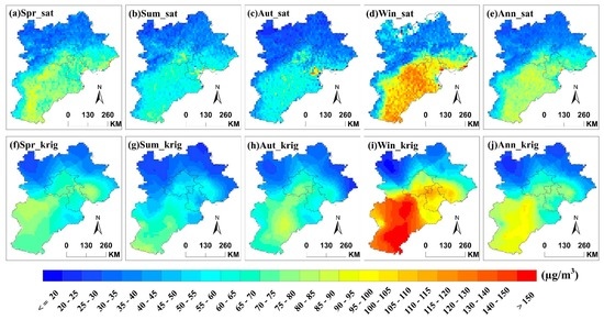
3.3. PM_2.5 Concentration Prediction Maps and Descriptive Statistics

To further evaluate the prediction performance of our RF models in spatial distribution and seasonal aspects for exposure risk estimation and other adhibitions, we generated 10 km² grids based on calculated daily PM_2.5 concentration values, and the averaged PM_2.5 concentrations were calculated by combining the daily pixel-based retrieval values, including both the Aqua and Terra satellite results for each season, as well as for the whole year. The prediction maps are shown in Figure 5. Lee et al. [52] compared remote sensing inversion methods with kriging interpolation, and their conclusion highlighted the feasible use of kriging, especially in the case of a dense distribution of monitoring stations. Although we used different retrieval methods, this provides a referential approach to validate our retrieval results to some extent. Thus, as a comparison, Figure 5 also presents the mean ground observations according to kriging interpolation results. For interpolation maps, we extracted the corresponding MODIS transit time of hourly measured PM_2.5 data consistent with the satellites’ normal flight; to reduce the MODIS-GEOS-sites matching error in temporal resolution, the spherical model was employed. Figure 6 shows the variation of the statistical results for each averaged satellite-derived image versus geostatistical kriging interpolation maps for more intuitive analysis.

Here, we compare these two sources of maps. The spatial distribution of PM_2.5 concentration in both maps over the whole region (Figure 5) show high values distributed in the middle and south plain area, while low values are spread over the northern mountainous region. The satellite-derived images provide more rich details and capture more spatial variations; they have more consistent distributions of the yearly averaged AOD images, and reproduce the terrain conditions well (compare this with Figure 1). However, the interpolation results only produce geographically continuous and smooth PM_2.5 concentration estimations over the region, and thus barely reflect the varied topographic features and some other conditions, especially in the southwest mountainous and plateau regions; this embodies the inherent weaknesses of the kriging method applied for PM_2.5 concentration estimation when there is a lack of nearby measurements.

The seasonal variations of PM_2.5 levels in the study area are pronounced. From the box plot in Figure 6, it can be seen that the average PM_2.5 concentration during the winter is significantly higher than that in other seasons in both the derived and interpolated maps, with PM_2.5 concentrations of 70.42 and 89.86 μg/m³, respectively. Wintertime heating by coal burning generates air pollution emissions, and complicated climatic conditions are considered to be the main reason for the highest pollution levels occurring during this season. The second-highest PM_2.5 concentrations are observed in spring, with mean values almost the same at 58 μg/m³ in the two maps. In the interpolation maps, summer has the lowest pollution level of 48.36 μg/m³ and autumn has a value of 55.39 μg/m³. In the retrieval maps, the trend is reversed, with the PM_2.5 concentrations in summer and autumn being 50.13 and 44.73 μg/m³ (the lowest concentration of the four seasons), respectively. The annual mean PM_2.5 concentrations are 56.69 and 62.97 μg/m³ in the retrieval and interpolation maps, respectively. Across the whole study area, the average PM_2.5 concentration is relatively higher in the kriging maps than that in the retrieval maps, and the differences between the concentration values of the inversion and interpolation maps in spring, summer, autumn, winter, and the whole year are about −0.57, 1.77, −10.66, −19.44, and −6.28 μg/m³, respectively; that is, the average differences between the comparison maps are far less for spring and summer than for autumn and winter. The marked discrepancy in both maps, and the distinct underestimation in our average retrieval results in autumn and winter may be attributed to the lack of PM_2.5 retrievals and the rarity of AOD observations on some days of heavy pollution. Another possibility is that the interpolation results are not the criterion, since the distribution of the monitoring sites are uneven in this area, being predominantly concentrated in the most polluted urban areas; thus, the kriging interpolation results may inevitably overestimate relatively clean areas wherein estimation points are distant from monitoring sites, or where regional ground observation data are lacking, especially during the most polluted seasons. From the box-plot in Figure 6, it can be seen that the ranges of the lower and upper whiskers for the retrieval maps are all relatively larger than those for the interpolation maps, and the outliers lie within the retrieval values. These findings suggest that our retrieval models might better capture the extreme values within a wide dynamic range. In winter, the box plot is comparatively tall, which reveals a remarkable spatial variability of the PM_2.5 concentration.

We also plotted the inversion maps for the Terra and Aqua satellites separately (data not shown), and the seasonal variations were found to be nearly the same using combined statistics. The retrieved average PM_2.5 concentration observed by the Terra satellite sensors is higher than those obtained from the Aqua satellite; the differences between the values obtained by the Terra and Aqua maps for spring, summer, autumn, winter, and the whole year, are about 17.02, 6.80, 13.78, 16.12, and 13.11 μg/m³, respectively.

4. Discussion

We compared the inversion results from the Terra and Aqua satellite sensors by individually training models. The results suggest that when using the same dataset and common training and testing methods, the RF model is consistently more effective than the other three algorithms, that is, OR, regression trees, and SVM. From an algorithm perspective, the conventional parametric models would be difficult to fit asymmetrical data, regression trees may lead to overfitting and need to be pruned to obtain more inductive trees, and the SVM algorithm has a relatively poor generalization ability and will also produce overfitting phenomenon [53]. For the RF technique, the need for few and insensitive tuning parameters make it user friendly for parameter optimization. Additionally, the RF algorithm is not prone to overfitting, even for higher characteristic dimensions [54,55]. The most essential ingredients can be selected through RF variable importance functions to construct more concise, readily interpreted, comprehensive, and high-accuracy models. Both the satisfactory performance in our model comparison and the advantages of RF prove it to be a promising method to provide more effective and accurate results for PM_2.5 inversion. For model comparison and validation, we divided our data into training set, validation set, and testing set, and conducted the 10 × 5 CV procedure, which provides a better model validation and reduces the random error.

Nevertheless, the disadvantages of this study should not be ignored. For one thing, the reported mean PM_2.5 spatial patterns cannot accurately reflect the seasonal variations in PM_2.5 concentration and are not representative of the corresponding seasons when compared to observed interpolation maps, and they especially underestimate the concentrations in autumn and winter. This is mainly caused by missing MODIS aerosol products. In November and December 2015, the BTH region and some other northern cities experienced particularly bad haze pollution episodes; during this period, extremely high AOD values in MODIS pixels were mistaken for clouds and therefore eliminated, which brought about marked underestimations in the autumn and winter average PM_2.5 concentration maps across the whole BTH region. The standard MODIS inversion algorithm also masks snow-covered grid cells, which may sharply decrease the available AOD samples in winter. The interpolation results used for comparison also have large errors, since the spatial heterogeneity distribution of PM_2.5 images are unreasonable when expressed as a simple statistical average. All of these factors explain some of the discrepancies between retrieved and observed PM_2.5 concentrations. Furthermore, the satellites transit only twice a day, and the time limitation in health-related air quality studies are obvious. We could convert hourly PM_2.5 concentrations monitored by the sites into 24-h averages, and other modeling datasets are kept as they were, to explore the difference between 24-h mean values applied in air quality and the approximately daily concentration retrieved in this study. The predictive power needs to be further improved for exposure assessment and environmental application.

We compared our predictive results with those of several previous publications using advanced multivariate, nonparametric machine learning algorithms, and by integrating ground observations, satellite products, and meteorological datasets to predict PM_2.5 concentrations. For example, Gupta et al. [31] used the ANN on three years of MODIS AOD data and meteorological analysis materials over the Southeastern United States to estimate PM_2.5 mass concentration, and obtained regression coefficients of 0.74 (hourly average) and 0.78 (daily mean). Additionally, Nguyen et al. [32] investigated the performance of MLR and SVM techniques applied for PM_1/2.5/10 prediction over a period from August 2010 to July 2012 over Hanoi, Vietnam; the results showed that SVM outperforms MLR and has a R and RMSE of 0.593 and 31.674, respectively in PM_2.5 concentration predictions. We obtained a higher correlation coefficient when using the SVM algorithm than those in the aforementioned literature results, let alone when using RF. Meanwhile, all of our models have a slightly higher RMSE than that of Nguyen’s results; the main reason for this is that the concentration is very high in our study domain, while the relatively low meteorological data precision and insufficient data size are also important reasons. Zheng et al. [56] predicted the annual average PM_2.5 concentration maps in three regions, including the BTH region, in 2013, and obtained a CV R² value of 0.77. Our model has a slightly lower precision, although it exhibited roughly similar spatial patterns compared with previous studies for the BTH region. The small precision discrepancy could mainly be attributed to the different choices of AOD products incorporated into the retrieval algorithm and quality assurance (QA) (we utilized the “AODcom” products with a mixed QA of 2 or 3, and this study used the DT AOD with a strict QA of 3).

Generally, our RF model has a promising prediction accuracy. It is possible to use higher-spatial-resolution materials to retrieve finer spatial patterns of PM_2.5 concentrations at regional and global scales, such as the MODIS Collection 6 aerosol products, which provide AOD retrievals with a spatial resolution of 3 km [57,58,59], and the multiangle implementation of the atmospheric correction algorithm (MAIAC), which infers the AOD retrievals at a spatial resolution of 1 km [60]. This strategy may also hold promise for multiyear applications, which could specifically provide further details regarding the spatial variation, to assess the acute and chronic epidemiological effects of PM_2.5 exposure, investigate the human exposure risk, and evaluate significant air quality events. The RF method can also be established for PM_2.5 pollution prediction based on long time-series.

In view of the abovementioned studies, the limitation of non-AOD retrieval days is the main obstacle of PM_2.5 concentration prediction in our study, particularly for heavy pollution conditions. Thus, further studies might place emphasis on improving the AOD spatial coverage. In particular, multiple-image data fusion is recommended as an effective method for improving the inversion algorithm of AOD. Missing data filling methods such as RF imputation also need to be explored and experimentally examined. Additionally, fusion algorithms combining remote sensing results with ground observation interpolation records would be a valuable direction for future research to not only improve the PM_2.5 coverage for high-pollution days near the measurement stations but also to improve the accuracy of inversion maps by uniting the advantages of both approaches.

5. Conclusions

In this study, we investigated the performance of OR, Rpart, SVM, and RF techniques for estimating the surface concentrations of PM_2.5 by aggregating MODIS aerosol products, GEOS meteorological parameters, and ground-based observations. The same training and testing datasets, as well as methods, were used for both the Terra and Aqua satellites in the BTH region for the year 2015, separately, to make all models entirely comparable. The 10-repeat 5-fold CV validation sets and the independent testing sets show that nonlinear and nonparametric methods are more efficient than the simple linear regression, and the ensemble machine learning models (SVM and RF) significantly improve the accuracy of PM_2.5 inversion. Furthermore, the RF methodology we introduced exhibited the best predictive results; combined with some valuable functions of the algorithm itself, the RF algorithm was shown to have a great potential for estimating ground-truth PM_2.5 observations. Additionally, due to the slightly varied data qualities for the individual satellites and daily distribution trend of PM_2.5, the Aqua satellite gives a more satisfactory prediction accuracy than the Terra satellite in all four models.

By applying the RF advanced machine learning algorithm, the retrieval of the daily PM_2.5 concentration at the time of MODIS passing over the territory in 2015, the spatiotemporal analysis compared with monitoring sites and kriging maps are performed simultaneously. The results show that the RF models with considerable improvement in inferring PM_2.5 concentration in space and time can basically reflect the spatial distribution of PM_2.5, and can be employed for human health studies where ground stations are very sparse or even unavailable, when the remotely-sensed aerosol data are not missing in great quantities.

References

1. Kioumourtzoglou, M.-A.; Schwartz, J.D.; Weisskopf, M.G.; Melly, S.J.; Wang, Y.; Dominici, F.; Zanobetti, A. Long-term PM2.5 Exposure and Neurological Hospital Admissions in the Northeastern United States. Environ. Health Perspect. 2016, 124, 23–29. [Google Scholar] [CrossRef] [PubMed]
2. Wellenius, G.A.; Bateson, T.F.; Mittleman, M.A.; Schwartz, J. Particulate air pollution and the rate of hospitalization for congestive heart failure among Medicare beneficiaries in Pittsburgh, Pennsylvania. Am. J. Epidemiol. 2005, 161, 1030–1036. [Google Scholar] [CrossRef] [PubMed]
3. Boldo, E.; Linares, C.; Lumbreras, J.; Borge, R.; Narros, A.; Garcia-Perez, J.; Fernandez-Navarro, P.; Perez-Gomez, B.; Aragones, N.; Ramis, R.; et al. Health impact assessment of a reduction in ambient PM2.5 levels in Spain. Environ. Int. 2011, 37, 342–348. [Google Scholar] [CrossRef] [PubMed]
4. Ostro, B.; Lipsett, M.; Reynolds, P.; Goldberg, D.; Hertz, A.; Garcia, C.; Henderson, K.D.; Bernstein, L. Long-Term Exposure to Constituents of Fine Particulate Air Pollution and Mortality: Results from the California Teachers Study. Environ. Health Perspect. 2010, 118, 363–369. [Google Scholar] [CrossRef] [PubMed] [Green Version]
5. Guo, J.-P.; Zhang, X.-Y.; Che, H.-Z.; Gong, S.-L.; An, X.; Cao, C.-X.; Guang, J.; Zhang, H.; Wang, Y.-Q.; Zhang, X.-C.; et al. Correlation between PM concentrations and aerosol optical depth in eastern China. Atmosp. Environ. 2009, 43, 5876–5886. [Google Scholar] [CrossRef]
6. Qi, Y.; Ge, J.; Huang, J. Spatial and temporal distribution of MODIS and MISR aerosol optical depth over northern China and comparison with AERONET. Chin. Sci. Bull. 2013, 58, 2497–2506. [Google Scholar] [CrossRef] [Green Version]
7. Sayer, A.M.; Hsu, N.C.; Bettenhausen, C.; Jeong, M.J.; Holben, B.N.; Zhang, J. Global and regional evaluation of over-land spectral aerosol optical depth retrievals from SeaWiFS. Atmosp. Meas. Tech. 2012, 5, 1761–1778. [Google Scholar] [CrossRef] [Green Version]
8. Xiao, Q.; Zhang, H.; Choi, M.; Li, S.; Kondragunta, S.; Kim, J.; Holben, B.; Levy, R.C.; Liu, Y. Evaluation of VIIRS, GOCI, and MODIS Collection 6AOD retrievals against ground sunphotometer observations over East Asia. Atmosp. Chem. Phys. 2016, 16, 1255–1269. [Google Scholar] [CrossRef]
9. Li, J.; Carlson, B.E.; Lacis, A.A. Application of spectral analysis techniques in the intercomparison of aerosol data: Part III. Using combined PCA to compare spatiotemporal variability of MODIS, MISR, and OMI aerosol optical depth. J. Geophys. Res.-Atmosp. 2014, 119, 4017–4042. [Google Scholar] [CrossRef] [Green Version]
10. Paciorek, C.J.; Liu, Y.; Moreno-Macias, H.; Kondragunta, S. Spatiotemporal associations between GOES aerosol optical depth retrievals and ground-level PM(2.5). Environ. Sci. Technol. 2008, 42, 5800–5806. [Google Scholar] [CrossRef]
11. Gupta, P.; Christopher, S.A. Particulate matter air quality assessment using integrated surface, satellite, and meteorological products: Multiple regression approach. J. Geophys. Res. 2009, 114. [Google Scholar] [CrossRef] [Green Version]
12. Liu, Y.; Park, R.J.; Jacob, D.J.; Li, Q.; Kilaru, V.; Sarnat, J.A. Mapping annual mean ground-level PM2.5 concentrations using Multiangle Imaging Spectroradiometer aerosol optical thickness over the contiguous United States. J. Geophys. Res. Atmosp. 2004, 109. [Google Scholar] [CrossRef]
13. Van Donkelaar, A.; Martin, R.V.; Park, R.J. Estimating ground-level PM2.5 using aerosol optical depth determined from satellite Remote Sensing. J. Geophys. Res. 2006, 111. [Google Scholar] [CrossRef]
14. Van Donkelaar, A.; Martin, R.V.; Spurr, R.J.D.; Drury, E.; Remer, L.A.; Levy, R.C.; Wang, J. Optimal estimation for global ground-level fine particulate matter concentrations. J. Geophys. Res.-Atmosp. 2013, 118, 5621–5636. [Google Scholar] [CrossRef] [Green Version]
15. Chu, D.A.; Tsai, T.-C.; Chen, J.-P.; Chang, S.-C.; Jeng, Y.-J.; Chiang, W.-L.; Lin, N.-H. Interpreting aerosol lidar profiles to better estimate surface PM2.5 for columnar AOD measurements. Atmosp. Environ. 2013, 79, 172–187. [Google Scholar] [CrossRef]
16. Lin, C.; Li, Y.; Yuan, Z.; Lau, A.K.H.; Li, C.; Fung, J.C.H. Using satellite Remote Sens. data to estimate the high-resolution distribution of ground-level PM2.5. Remote Sens. Environ. 2015, 156, 117–128. [Google Scholar] [CrossRef]
17. Zhang, Y.; Li, Z. Remote Sens. of atmospheric fine particulate matter (PM2.5) mass concentration near the ground from satellite observation. Remote Sens. Environ. 2015, 160, 252–262. [Google Scholar] [CrossRef]
18. Gardner, M.W.; Dorling, S.R. Artificial neural networks (the multilayer perceptron)—A review of applications in the atmospheric sciences. Atmosp. Environ. 1998, 32, 2627–2636. [Google Scholar] [CrossRef]
19. Wang, J. Intercomparison between satellite-derived aerosol optical thickness and PM2.5 mass: Implications for air quality studies. Geophys. Res. Lett. 2003, 30. [Google Scholar] [CrossRef]
20. Zhang, Z.; Wang, X.; Li, B.; Hou, Y.; Yang, J.; Yi, L. Development of a novel morphological paclitaxel-loaded PLGA microspheres for effective cancer therapy: In vitro and in vivo evaluations. Drug Deliv. 2018, 25, 166–177. [Google Scholar] [CrossRef]
21. Liu, Y.; Sarnat, J.A.; Kilaru, V.; Jacob, D.J.; Koutrakis, P. Estimating Ground-Level PM2.5 in the Eastern United States Using Satellite Remote Sensing. Environ. Sci. Technol. 2005, 39, 3269–3278. [Google Scholar] [CrossRef] [PubMed]
22. Beckerman, B.S.; Jerrett, M.; Serre, M.; Martin, R.V.; Lee, S.J.; van Donkelaar, A.; Ross, Z.; Su, J.; Burnett, R.T. A hybrid approach to estimating national scale spatiotemporal variability of PM2.5 in the contiguous United States. Environ. Sci. Technol. 2013, 47, 7233–7241. [Google Scholar] [CrossRef] [PubMed]
23. Hu, X.; Waller, L.A.; Al-Hamdan, M.Z.; Crosson, W.L.; Estes, M.G., Jr.; Estes, S.M.; Quattrochi, D.A.; Sarnat, J.A.; Liu, Y. Estimating ground-level PM(2.5) concentrations in the southeastern U.S. using geographically weighted regression. Environ. Res. 2013, 121, 1–10. [Google Scholar] [CrossRef] [PubMed]
24. Jiang, M.; Sun, W.; Yang, G.; Zhang, D. Modelling Seasonal GWR of Daily PM2.5 with Proper Auxiliary Variables for the Yangtze River Delta. Remote Sens. 2017, 9, 346. [Google Scholar] [CrossRef]
25. Ma, Z.; Hu, X.; Huang, L.; Bi, J.; Liu, Y. Estimating ground-level PM2.5 in China using satellite Remote Sensing. Environ. Sci. Technol. 2014, 48, 7436–7444. [Google Scholar] [CrossRef] [PubMed]
26. You, W.; Zang, Z.; Zhang, L.; Li, Y.; Pan, X.; Wang, W. National-Scale Estimates of Ground-Level PM2.5 Concentration in China Using Geographically Weighted Regression Based on 3 km Resolution MODIS AOD. Remote Sens. 2016, 8, 184. [Google Scholar] [CrossRef]
27. Bai, Y.; Wu, L.; Qin, K.; Zhang, Y.; Shen, Y.; Zhou, Y. A Geographically and Temporally Weighted Regression Model for Ground-Level PM2.5 Estimation from Satellite-Derived 500 m Resolution AOD. Remote Sens. 2016, 8, 262. [Google Scholar] [CrossRef]
28. Hu, X.; Waller, L.A.; Lyapustin, A.; Wang, Y.; Liu, Y. 10-year spatial and temporal trends of PM2.5 concentrations in the southeastern US estimated using high-resolution satellite data. Atmos Chem. Phys. 2014, 14, 6301–6314. [Google Scholar] [CrossRef]
29. Chuang, Y.-H.; Mazumdar, S.; Park, T.; Tang, G.; Arena, V.C.; Nicolich, M.J. Generalized linear mixed models in time series studies of air pollution. Atmosp. Pollut. Res. 2011, 2, 428–435. [Google Scholar] [CrossRef]
30. Liang, F.; Xiao, Q.; Wang, Y.; Lyapustin, A.; Li, G.; Gu, D.; Pan, X.; Liu, Y. MAIAC-based long-term spatiotemporal trends of PM2.5 in Beijing, China. Sci. Total Environ. 2018, 616, 1589–1598. [Google Scholar] [CrossRef]
31. Gupta, P.; Christopher, S.A. Particulate matter air quality assessment using integrated surface, satellite, and meteorological products: 2. A neural network approach. J. Geophys. Res. 2009, 114. [Google Scholar] [CrossRef] [Green Version]
32. Nguyen, T.N.T.; Ta, V.C.; Le, T.H.; Mantovani, S. Particulate Matter Concentration Estimation from Satellite Aerosol and Meteorological Parameters: Data-Driven Approaches. Knowl. Syst. Eng. 2014, 244, 351–362. [Google Scholar] [CrossRef]
33. Sorek-Hamer, M.; Strawa, A.W.; Chatfield, R.B.; Esswein, R.; Cohen, A.; Broday, D.M. Improved retrieval of PM2.5 from satellite data products using non-linear methods. Environ. Pollut. 2013, 182, 417–423. [Google Scholar] [CrossRef] [PubMed]
34. Huang, K.; Xiao, Q.; Meng, X.; Geng, G.; Wang, Y.; Lyapustin, A.; Gu, D.; Liu, Y. Predicting monthly high-resolution PM2.5 concentrations with random forest model in the North China Plain. Environ. Pollut. 2018, 242, 675–683. [Google Scholar] [CrossRef] [PubMed]
35. Yu, R.; Yang, Y.; Yang, L.; Han, G.; Move, O.A. RAQ-A Random Forest Approach for Predicting Air Quality in Urban Sensing Systems. Sensors 2016, 16, 86. [Google Scholar] [CrossRef] [PubMed]
36. Isobe, T.; Feigelson, E.D.; Akritas, M.G.; Babu, G.J. Linear-Regression in Astronomy. I. Astrophys. J. 1990, 364, 104–113. [Google Scholar] [CrossRef]
37. Gass, K.; Klein, M.; Chang, H.H.; Flanders, W.D.; Strickland, M.J. Classification and regression trees for epidemiologic research: An air pollution example. Environ. Health 2014, 13. [Google Scholar] [CrossRef] [PubMed]
38. Levy, R.C.; Mattoo, S.; Munchak, L.A.; Remer, L.A.; Sayer, A.M.; Patadia, F.; Hsu, N.C. The Collection 6 MODIS aerosol products over land and ocean. Atmosp. Meas. Tech. 2013, 6, 2989–3034. [Google Scholar] [CrossRef] [Green Version]
39. Sayer, A.M.; Munchak, L.A.; Hsu, N.C.; Levy, R.C.; Bettenhausen, C.; Jeong, M.J. MODIS Collection 6 aerosol products: Comparison between Aqua’s e-Deep Blue, Dark Target, and “merged” data sets, and usage recommendations. J. Geophys. Res.-Atmosp. 2014, 119, 13965–13989. [Google Scholar] [CrossRef]
40. Lee, H.J.; Liu, Y.; Coull, B.A.; Schwartz, J.; Koutrakis, P. A novel calibration approach of MODIS AOD data to predict PM2.5 concentrations. Atmosp. Chem. Phys. Discuss. 2011, 11, 9769–9795. [Google Scholar] [CrossRef]
41. Oleson, J.J.; Kumar, N.; Smith, B.J. Spatiotemporal modeling of irregularly spaced Aerosol Optical Depth data. Environ. Ecol. Stat. 2013, 20, 297–314. [Google Scholar] [CrossRef] [PubMed]
42. Cantrell, C.A. Technical Note: Review of methods for linear least-squares fitting of data and application to atmospheric chemistry problems. Atmosp. Chem. Phys. 2008, 8, 5477–5487. [Google Scholar] [CrossRef]
43. Wu, C.; Yu, J.Z. Evaluation of linear regression techniques for atmospheric applications: The importance of appropriate weighting. Atmosp. Meas. Tech. 2018, 11, 1233–1250. [Google Scholar] [CrossRef]
44. De’ath, G.; Fabricius, K.E. Classification and regression trees: A powerful yet simple technique for ecological data analysis. Ecology 2000, 81, 3178–3192. [Google Scholar] [CrossRef]
45. Breiman, L. Random forests. Mach. Learn. 2001, 45, 5–32. [Google Scholar] [CrossRef]
46. Campbell, C. Kernel methods: A survey of current techniques. Neurocomputing 2002, 48, 63–84. [Google Scholar] [CrossRef]
47. Chang, C.C.; Lin, C.J. Training nu-support vector regression: Theory and algorithms. Neural Comput. 2002, 14, 1959–1977. [Google Scholar] [CrossRef]
48. Chang, C.-C.; Lin, C.-J. LIBSVM: A Library for Support Vector Machines. Acm Trans. Intell. Syst. Technol. 2011, 2. [Google Scholar] [CrossRef]
49. Mahmood, Z.; Khan, S. On the Use of K-Fold Cross-Validation to Choose Cutoff Values and Assess the Performance of Predictive Models in Stepwise Regression. Int. J. Biostat. 2009, 5. [Google Scholar] [CrossRef] [Green Version]
50. Levy, R.C.; Mattoo, S.; Sawyer, V.; Shi, Y.; Colarco, P.R.; Lyapustin, A.I.; Wang, Y.; Remer, L.A. Exploring systematic offsets between aerosol products from the two MODIS sensors. Atmosp. Meas. Tech. 2018, 11, 4073–4092. [Google Scholar] [CrossRef]
51. Kuhn, S.; Egert, B.; Neumann, S.; Steinbeck, C. Building blocks for automated elucidation of metabolites: Machine learning methods for NMR prediction. Bmc Bioinform. 2008, 9. [Google Scholar] [CrossRef] [PubMed]
52. Lee, S.J.; Serre, M.L.; van Donkelaar, A.; Martin, R.V.; Burnett, R.T.; Jerrett, M. Comparison of geostatistical interpolation and Remote Sens. techniques for estimating long-term exposure to ambient PM2.5 concentrations across the continental United States. Environ. Health Perspect. 2012, 120, 1727–1732. [Google Scholar] [CrossRef] [PubMed]
53. Wu, X.; Kumar, V.; Ross Quinlan, J.; Ghosh, J.; Yang, Q.; Motoda, H.; McLachlan, G.J.; Ng, A.; Liu, B.; Yu, P.S.; et al. Top 10 algorithms in data mining. Knowl. Inf. Syst. 2007, 14, 1–37. [Google Scholar] [CrossRef] [Green Version]
54. Li, X.; Sha, J.; Wang, Z.-L. Application of feature selection and regression models for chlorophyll-a prediction in a shallow lake. Environ. Sci. Pollut. Res. 2018, 25, 19488–19498. [Google Scholar] [CrossRef] [PubMed]
55. Markovic, R.; Wolf, S.; Cao, J.; Spinnraker, E.; Wolki, D.; Frisch, J.; van Treeck, C. Comparison of Different Classification Algorithms for the Detection of User’s Interaction with Windows in Office Buildings. In Proceedings of the Cisbat 2017 International Conference Future Buildings & Districts-Energy Efficiency from Nano to Urban Scale, Lausanne, Switzerland, 6–8 September 2017; Volume 122, pp. 337–342. [Google Scholar]
56. Zheng, Y.; Zhang, Q.; Liu, Y.; Geng, G.; He, K. Estimating ground-level PM2.5 concentrations over three megalopolises in China using satellite-derived aerosol optical depth measurements. Atmosp. Environ. 2016, 124, 232–242. [Google Scholar] [CrossRef]
57. Ma, Q.; Li, Y.; Liu, J.; Chen, J.M. Long Temporal Analysis of 3-km MODIS Aerosol Product Over East China. IEEE J. Sel. Top. Appl. Earth Observ. Remote Sens. 2017, 10, 2478–2490. [Google Scholar] [CrossRef]
58. Nichol, J.E.; Bilal, M. Validation of MODIS 3 km Resolution Aerosol Optical Depth Retrievals Over Asia. Remote Sens. 2016, 8, 328. [Google Scholar] [CrossRef]
59. Remer, L.A.; Mattoo, S.; Levy, R.C.; Munchak, L.A. MODIS 3 km aerosol product: Algorithm and global perspective. Atmosp. Meas. Tech. 2013, 6, 1829–1844. [Google Scholar] [CrossRef]
60. Lyapustin, A.; Wang, Y.; Laszlo, I.; Kahn, R.; Korkin, S.; Remer, L.; Levy, R.; Reid, J.S. Multiangle implementation of atmospheric correction (MAIAC): 2. Aerosol algorithm. J. Geophys. Res. 2011, 116. [Google Scholar] [CrossRef] [Green Version]
Figure 1. Topography and spatial distribution of PM2.5 monitoring stations (upper-right) and annual mean “AODcom” maps (bottom-left for the Terra satellite and bottom-right for the Aqua satellite) of the Beijing–Tianjin–Hebei (BTH) region. A histogram equalization contrast stretch was applied in these maps.
Remotesensing 10 02006 g001
Figure 2. Scatterplots of observed and predicted concentrations of PM2.5 in test sets for all models. The solid line shows the fitted models for observed and predicted PM2.5 concentrations. The dashed line is the reference (y = x).
Remotesensing 10 02006 g002
Figure 3. The importance of RF variables (left) and the correlation coefficients between variables and PM2.5 concentration (right).
Remotesensing 10 02006 g003
Figure 4. Examples of time-series validation for MOD- (Terra satellite; left) and MYD (Aqua satellite; right)-derived PM2.5 concentrations for in-site observations and RF-model-based estimations for three stations in the Beijing–Tianjin–Hebei (BTH) region using all available days. The three horizontal dashed lines from bottom to top in each panel represent the concentration levels of 15 µg/m3, 35 µg/m3, and 75 µg/m3, respectively.
Remotesensing 10 02006 g004
Figure 5. PM2.5 concentration prediction maps based on RF invention (ae) and kriging interpolation (fj). Spr, Sum, Aut, Win, and Ann represent spring, summer, autumn, winter, and the whole year, respectively.
Remotesensing 10 02006 g005
Figure 6. Statistical results of derived (_sat) and interpolated (_krig) PM2.5 concentration maps. The mean values are shown as red circles, and the median marks and the midpoint are shown by the lines. The upper and lower quartiles (75th and 25th quantiles) represent 75% and 25% of the data, respectively, and the upper and lower whiskers represent the locations of the minima and maxima. Outliers are represented by black circles.
Remotesensing 10 02006 g006