Evaluation of Unsupervised Change Detection Methods Applied to Landslide Inventory Mapping Using ASTER Imagery

 , ,
, ,  ,
,
Abstract
1. Introduction
2. Study Area and Dataset
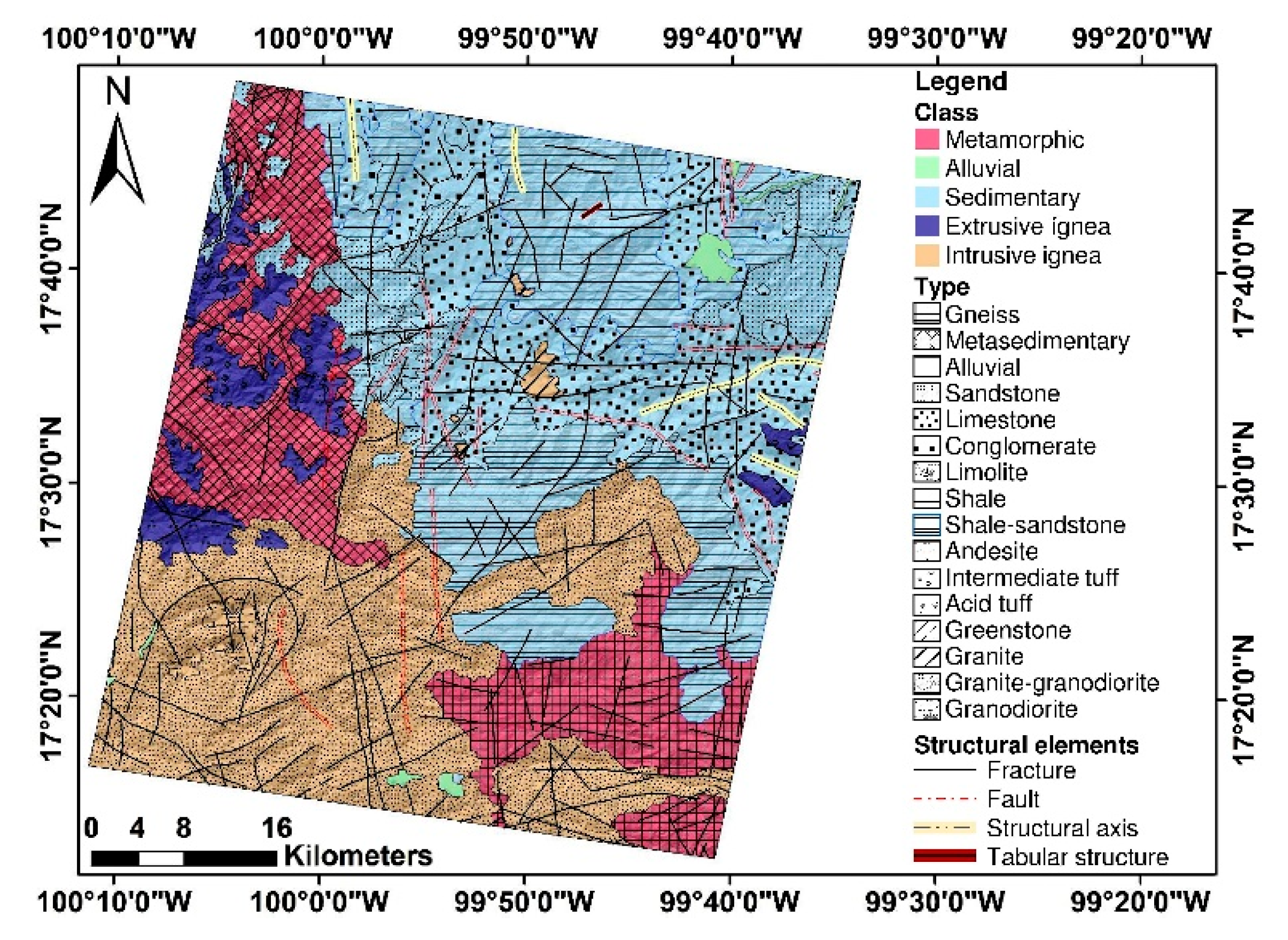
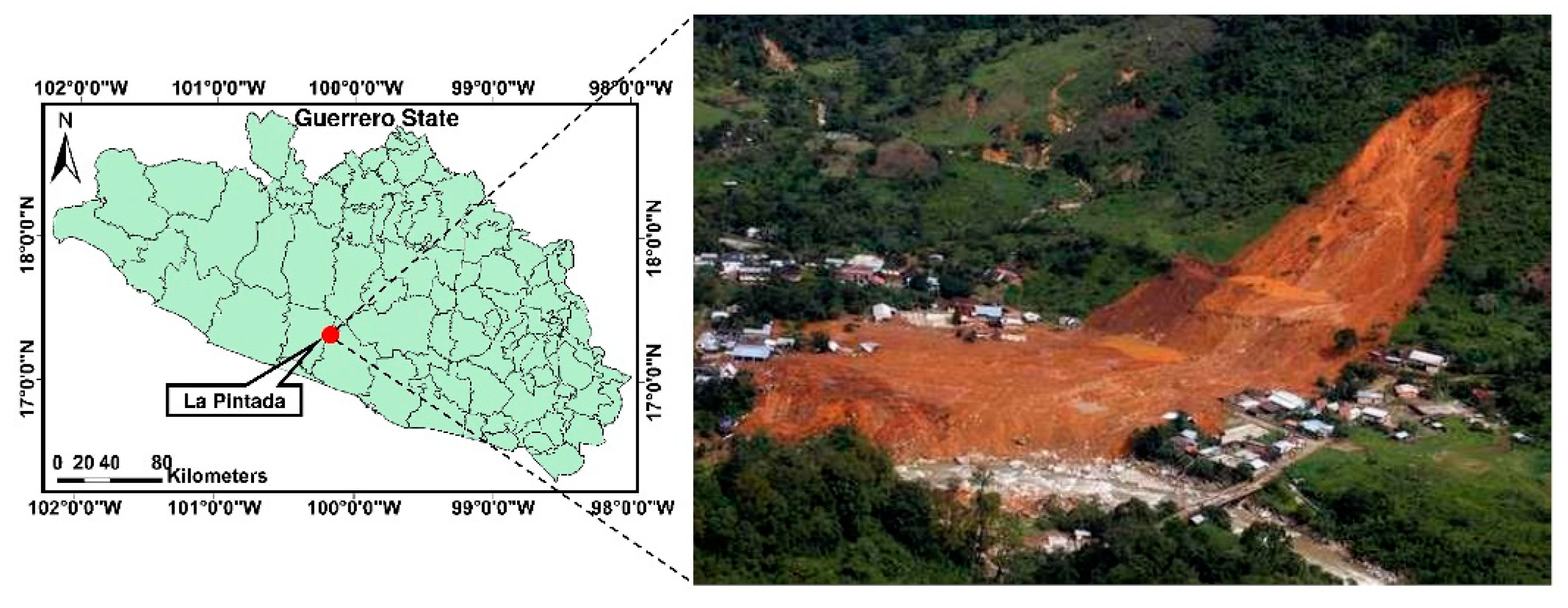
2.1. Study Area
2.2. Dataset
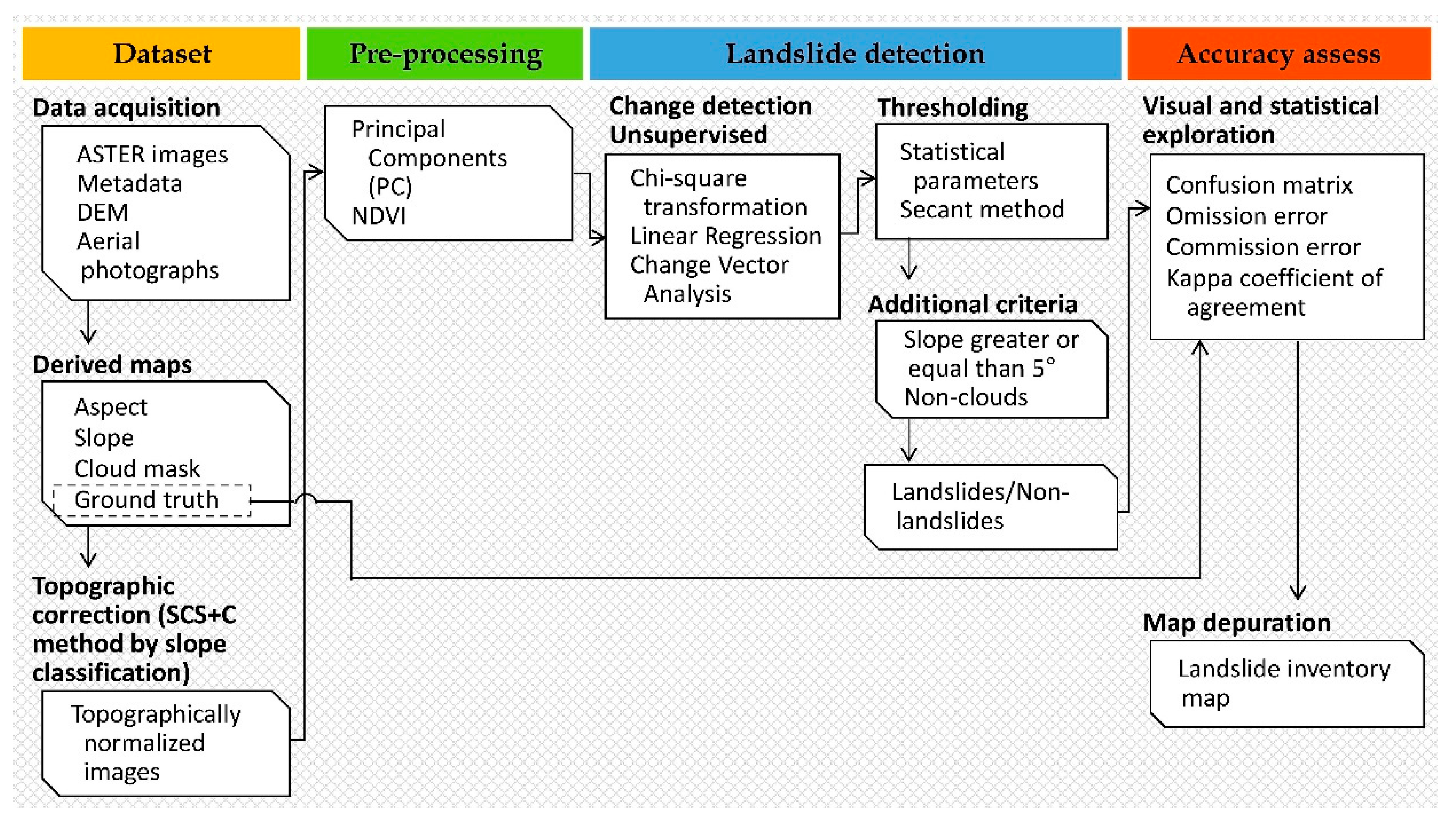
3. Methods
3.1. Topographic Normalization
3.2. Pre-Processing
3.3. Change Detection
3.3.1. Chi-Square Transformation
3.3.2. Linear Regression
3.3.3. Change Vector Analysis
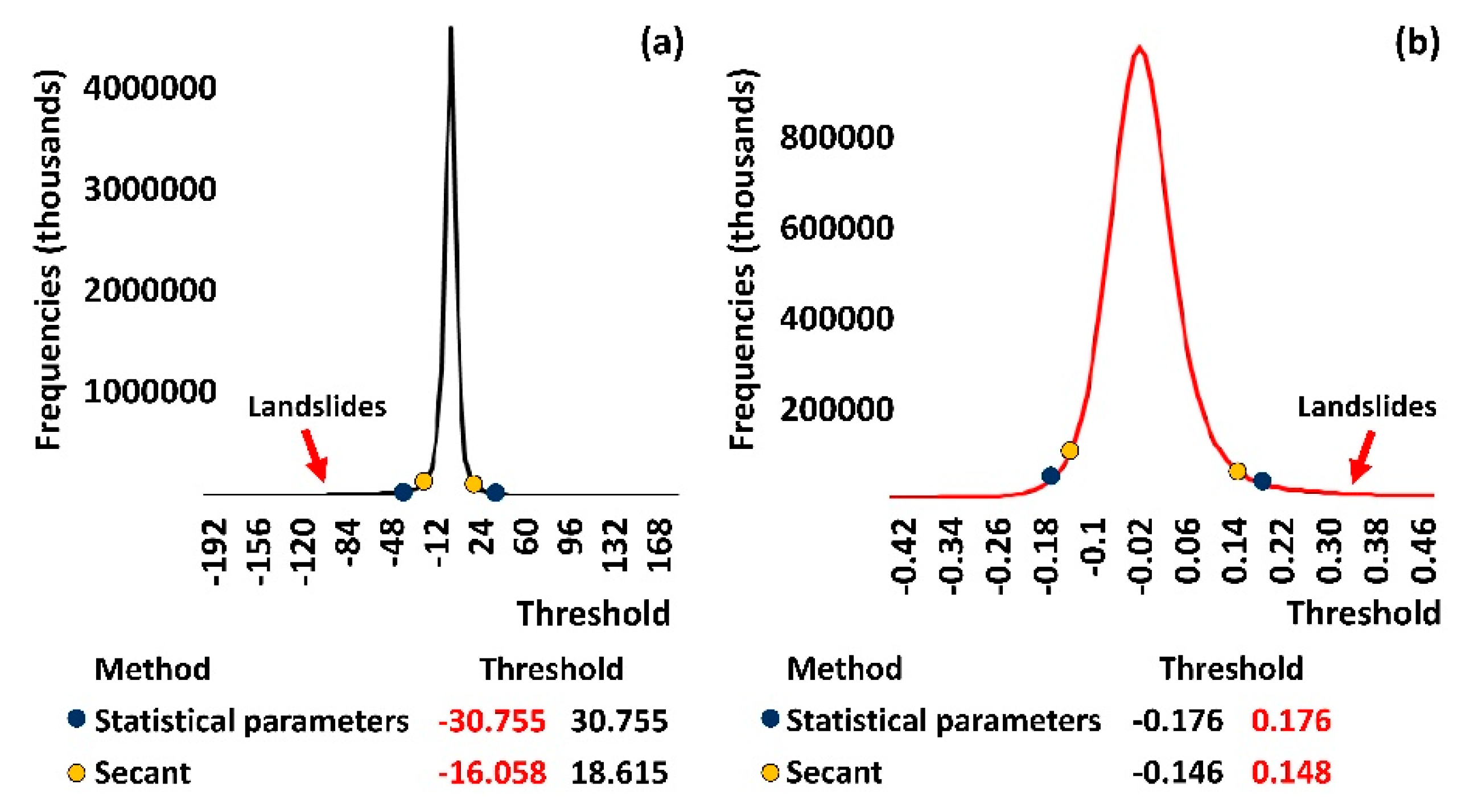
3.4. Threshold Definition
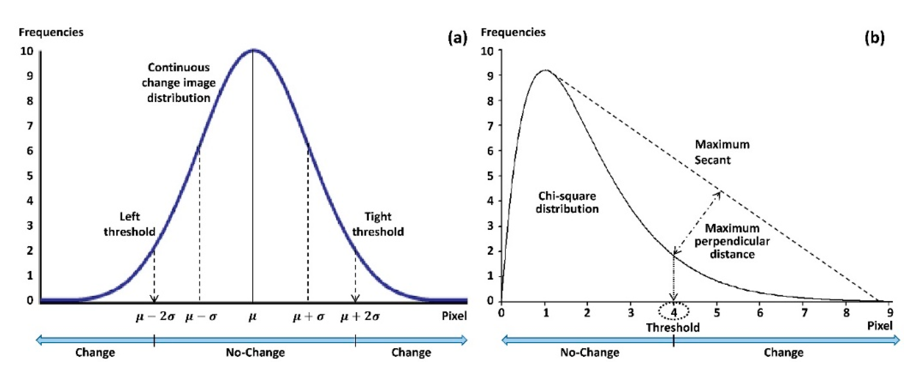
3.4.1. Statistical Thresholding Method
3.4.2. Secant Thresholding Method
3.5. Accuracy Assessment
3.6. Integration of the Final Landslide Map Inventory
4. Results
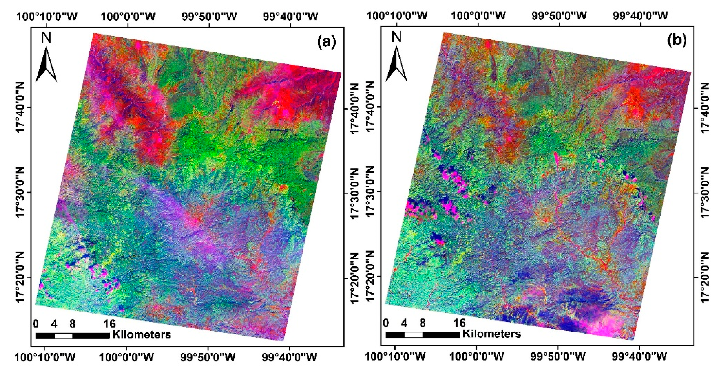
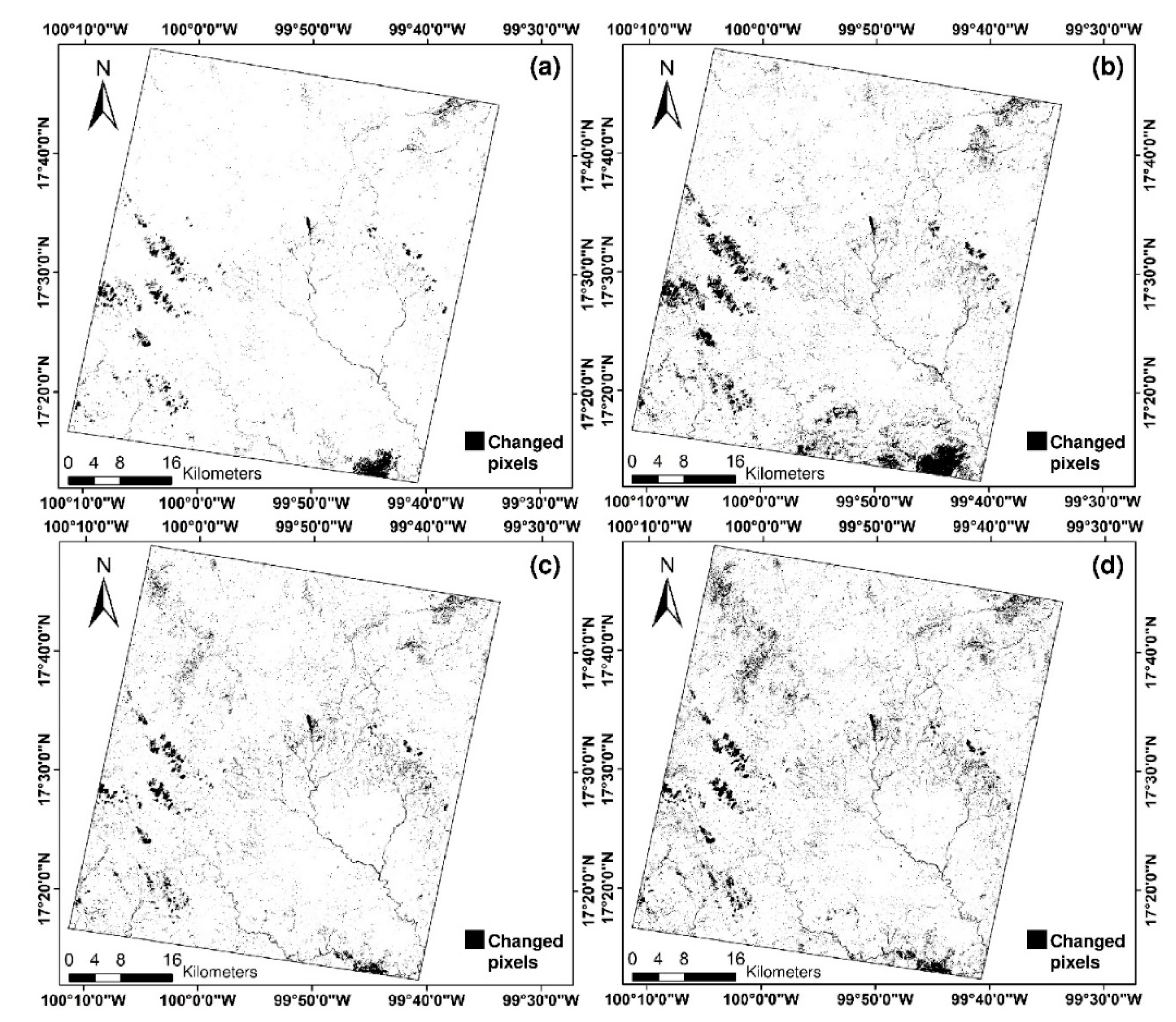
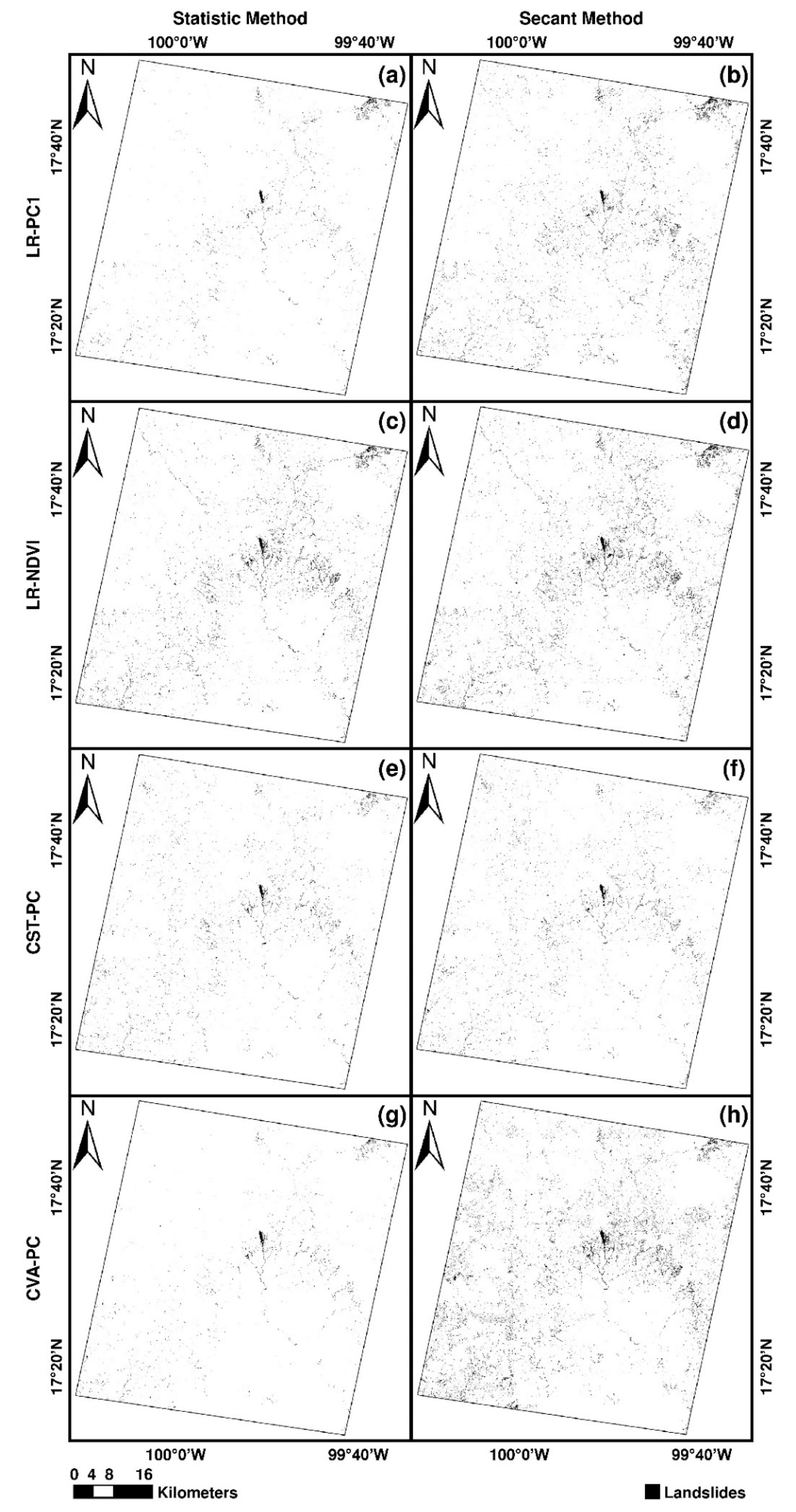
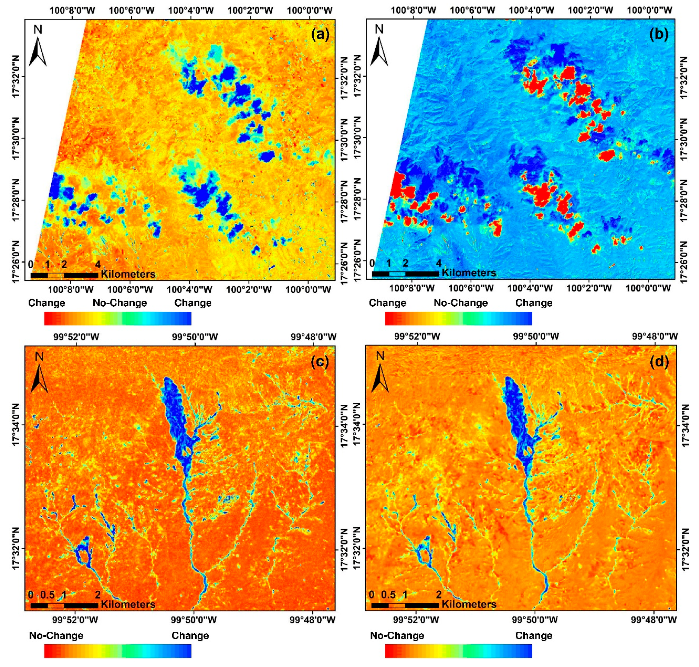
4.1. Change Detection Maps
4.2. Threshold Definition
4.3. Accuracy Assessment
4.4. Final Landslide Inventory Map
5. Discussion
5.1. Change Detection Maps
5.2. Threshold Definition
5.3. Accuracy Assessment
5.4. Final Landslide Inventory Map
6. Conclusions
Author Contributions
Funding
Acknowledgments
Conflicts of Interest
References
- Van Westen, C.; Van Asch, T.W.; Soeters, R. Landslide hazard and risk zonation—Why is it still so difficult? Bull. Eng. Geol. Environ. 2006, 65, 167–184. [Google Scholar] [CrossRef]
- Wirtz, A.; Kron, W.; Löw, P.; Steuer, M. The need for data: Natural disasters and the challenges of database management. Nat. Hazards 2014, 70, 135–157. [Google Scholar] [CrossRef]
- Chen, T.; Niu, R.; Du, B.; Wang, Y. Landslide spatial susceptibility mapping by using GIS and remote sensing techniques: A case study in Zigui County, the Three Georges reservoir, China. Environ. Earth Sci. 2015, 73, 5571–5583. [Google Scholar] [CrossRef]
- Ramos-Bernal, R.N.; Vázquez-Jiménez, R.; Romero-Rojas, W. Modeling the Susceptibility to Landslides by Remote Sensing Techniques. Case Study: Central Area of the State of Guerrero in México, Havana, Cuba, 22-04-2018; Ministerio de Comunicaciones: Havana, Cuba, 2018; pp. 1–8. ISBN 978-959-7255-00-0. [Google Scholar]
- Guzzetti, F.; Cardinali, M.; Reichenbach, P.; Carrara, A. Comparing landslide maps: A case study in the upper Tiber River Basin, central Italy. Environ. Manag. 2000, 25, 247–263. [Google Scholar] [CrossRef]
- IPCC. Managing the Risks of Extreme Events and Disasters to Advance Climate Change Adaptation: Special Report of the Intergovernmental Panel on Climate Change. A Special Report of Working Groups I and II of the Intergovernmental Panel on Climate Change; Cambridge University Press: Cambridge, UK; New York, NY, USA, 2012; pp. 1–19. [Google Scholar]
- Poursanidis, D.; Chrysoulakis, N. Remote Sensing, Natural Hazards and the contribution of ESA Sentinels missions. Remote Sens. Appl. Soc. Environ. 2017, 6, 25–38. [Google Scholar] [CrossRef]
- CRED-UNISDR. 2015 Disasters in Numbers; United Nations Office for Disaster Risk Reduction: Geneva, Switzerland, 2016; pp. 1–2. [Google Scholar]
- Pereira, S.; Zêzere, J.L.; Quaresma, I.D.; Bateira, C. Landslide incidence in the North of Portugal: Analysis of a historical landslide database based on press releases and technical reports. Geomorphology 2014, 214, 514–525. [Google Scholar] [CrossRef]
- Ciampalini, A.; Raspini, F.; Bianchini, S.; Frodella, W.; Bardi, F.; Lagomarsino, D.; Di Traglia, F.; Moretti, S.; Proietti, C.; Pagliara, P. Remote sensing as tool for development of landslide databases: The case of the Messina Province (Italy) geodatabase. Geomorphology 2015, 249, 103–118. [Google Scholar] [CrossRef]
- Rosi, A.; Tofani, V.; Tanteri, L.; Stefanelli, C.T.; Agostini, A.; Catani, F.; Casagli, N. The new landslide inventory of Tuscany (Italy) updated with PS-InSAR: Geomorphological features and landslide distribution. Landslides 2018, 15, 5–19. [Google Scholar] [CrossRef]
- Harp, E.L.; Jibson, R.W. Landslides triggered by the 1994 Northridge, California, earthquake. Bull. Seismol. Soc. Am. 1996, 86, S319–S332. [Google Scholar]
- Cardinali, M.; Ardizzone, F.; Galli, M.; Guzzetti, F.; Reichenbach, P. Landslides triggered by rapid snow melting: The December 1996–January 1997 event in Central Italy. In Proceedings of the 1st Plinius Conference on Mediterranean Storms, Maratea, Italy, 14–16 October 1999; pp. 439–448. [Google Scholar]
- Bucknam, R.C.; Coe, J.A.; Chavarría, M.M.; Godt, J.W.; Tarr, A.C.; Bradley, L.; Rafferty, S.; Hancock, D.; Dart, R.L.; Johnson, M.L. Landslides Triggered by Hurricane Mitch in Guatemala–Inventory and Discussion; US Geological Survey Open File Report 01-443; USGS: Denver, Colorado, 2001; Volume 1, p. 38. [Google Scholar] [CrossRef]
- Malamud, B.D.; Turcotte, D.L.; Guzzetti, F.; Reichenbach, P. Landslide inventories and their statistical properties. Earth Surf. Process. Landf. 2004, 29, 687–711. [Google Scholar] [CrossRef]
- Chung, C.F.; Fabbri, A.G. Systematic procedures of landslide hazard mapping for risk assessment using spatial prediction models. In Landslide Risk Assessment; Glade, T., Anderson, M., Crozier, M.J., Eds.; John Wiley: Hoboken, NJ, USA, 2005; pp. 139–174. [Google Scholar]
- Guzzetti, F.; Galli, M.; Reichenbach, P.; Ardizzone, F.; Cardinali, M. Landslide hazard assessment in the Collazzone area, Umbria, Central Italy. Nat. Hazards Earth Syst. Sci. 2006, 6, 115–131. [Google Scholar] [CrossRef]
- Mezaal, M.; Pradhan, B.; Rizeei, H. Improving Landslide Detection from Airborne Laser Scanning Data Using Optimized Dempster–Shafer. Remote Sens. 2018, 10, 1029. [Google Scholar] [CrossRef]
- Liu, X.; Zhao, C.; Zhang, Q.; Peng, J.; Zhu, W.; Lu, Z. Multi-Temporal Loess Landslide Inventory Mapping with C-, X-and L-Band SAR Datasets—A Case Study of Heifangtai Loess Landslides, China. Remote Sens. 2018, 10, 1756. [Google Scholar] [CrossRef]
- Xiaodong, Z.; Ya, G.; Deren, L. A strategy of change detection based on remotely sensed imagery and GIS data. In Proceedings of the ISPRS Commission. VII Symposium “Remote Sensing: From Pixels to Proceses”, Enschede, The Netherlands, 8–11 May 2006. [Google Scholar]
- Zanchetta, A.; Bitelli, G.; Karnieli, A. Monitoring desertification by remote sensing using the Tasselled Cap transform for long-term change detection. Nat. Hazards 2016, 83, 223–237. [Google Scholar] [CrossRef]
- Zhang, P.; Gong, M.; Su, L.; Liu, J.; Li, Z. Change detection based on deep feature representation and mapping transformation for multi-spatial-resolution remote sensing images. ISPRS J. Photogramm. Remote Sens. 2016, 116, 24–41. [Google Scholar] [CrossRef]
- Guzzetti, F.; Mondini, A.C.; Cardinali, M.; Fiorucci, F.; Santangelo, M.; Chang, K. Landslide inventory maps: New tools for an old problem. Earth-Sci. Rev. 2012, 112, 42–66. [Google Scholar] [CrossRef]
- Hervás, J.; Bobrowsky, P. Mapping: Inventories, susceptibility, hazard and risk. In Landslides–Disaster Risk Reduction; Springer: New York, NY, USA, 2009; pp. 321–349. [Google Scholar]
- Van Den Eeckhaut, M.; Poesen, J.; Verstraeten, G.; Vanacker, V.; Moeyersons, J.; Nyssen, J.; Van Beek, L. The effectiveness of hillshade maps and expert knowledge in mapping old deep-seated landslides. Geomorphology 2005, 67, 351–363. [Google Scholar] [CrossRef]
- Mantovani, F.; Soeters, R.; Van Westen, C. Remote sensing techniques for landslide studies and hazard zonation in Europe. Geomorphology 1996, 15, 213–225. [Google Scholar] [CrossRef]
- Metternicht, G.; Hurni, L.; Gogu, R. Remote sensing of landslides: An analysis of the potential contribution to geo-spatial systems for hazard assessment in mountainous environments. Remote Sens. Environ. 2005, 98, 284–303. [Google Scholar] [CrossRef]
- Singhroy, V.; Molch, K. Characterizing and monitoring rockslides from SAR techniques. Adv. Space Res. 2004, 33, 290–295. [Google Scholar] [CrossRef]
- Singhroy, V. Landslide Hazards: CEOS, the Use of Earth Observing Satellites for Hazard Support: Assessments and Scenarios; Final Report of the CEOS Disaster Management Support Group; NOAA: Silver Spring, MD, USA, 2002; p. 98. [Google Scholar]
- Singhroy, V.; Mattar, K.; Gray, A. Landslide characterisation in Canada using interferometric SAR and combined SAR and TM images. Adv. Space Res. 1998, 21, 465–476. [Google Scholar] [CrossRef]
- Gupta, R.; Saha, A. Mapping Debris Flows in the Himalayas, Natural Resource Management. GEOSPATIALWORLD 2001, 4. Available online: https://www.geospatialworld.net/article/mapping-debris-flows-in-the-himalayas/ (accessed on 26 November 2018).
- Cheng, K.; Wei, C.; Chang, S. Locating landslides using multi-temporal satellite images. Adv. Space Res. 2004, 33, 296–301. [Google Scholar] [CrossRef]
- Aksoy, B.; Ercanoglu, M. Landslide identification and classification by object-based image analysis and fuzzy logic: An example from the Azdavay region (Kastamonu, Turkey). Comput. Geosci. 2012, 38, 87–98. [Google Scholar] [CrossRef]
- Rau, J.; Jhan, J.; Rau, R. Semiautomatic object-oriented landslide recognition scheme from multisensor optical imagery and DEM. IEEE Trans. Geosci. Remote Sens. 2014, 52, 1336–1349. [Google Scholar] [CrossRef]
- Pour, A.B.; Hashim, M. Application of Landsat-8 and ALOS-2 data for structural and landslide hazard mapping in Kelantan, Malaysia. Nat. Hazards Earth Syst. Sci. 2017, 17, 1285–1303. [Google Scholar] [CrossRef]
- Hashim, M.; Misbari, S.; Pour, A.B. Landslide mapping and assessment by integrating Landsat-8, PALSAR-2 and GIS techniques: A case study from kelantan state, peninsular Malaysia. J. Indian Soc. Remote Sens. 2018, 46, 233–248. [Google Scholar] [CrossRef]
- Si, A.; Zhang, J.; Tong, S.; Lai, Q.; Wang, R.; Li, N.; Bao, Y. Regional Landslide Identification Based on Susceptibility Analysis and Change Detection. ISPRS Int. J. Geo-Inf. 2018, 7, 394. [Google Scholar] [CrossRef]
- Singh, A. Review article digital change detection techniques using remotely-sensed data. Int. J. Remote Sens. 1989, 10, 989–1003. [Google Scholar] [CrossRef]
- Wang, Q.; Atkinson, P.M.; Shi, W. Fast subpixel mapping algorithms for subpixel resolution change detection. IEEE Trans. Geosci. Remote Sens. 2015, 53, 1692–1706. [Google Scholar] [CrossRef]
- Vázquez-Jiménez, R.; Romero-Calcerrada, R.; Novillo, C.J.; Ramos-Bernal, R.N.; Arrogante Funes, P. Applying the Chi-square transformation and automatic secant thresholding to Landsat imagery as unsupervised change detection methods. J. Appl. Remote Sens. 2017, 11, 1–14. [Google Scholar] [CrossRef]
- Mas, J. Monitoring land-cover changes: A comparison of change detection techniques. Int. J. Remote Sens. 1999, 20, 139–152. [Google Scholar] [CrossRef]
- Xu, L.; Zhang, S.; He, Z.; Guo, Y. The comparative study of three methods of remote sensing image change detection. Int. Arch. Photogramm. Remote Sens. Spat. Inf. Sci. 2008, 37, 1595–1598. [Google Scholar] [CrossRef]
- Chuvieco, E. Teledetección Ambiental: La Observación de la Tierra Desde el Espacio, 1st ed.; Ariel: Madrid, Spain, 2010; p. 591. [Google Scholar]
- Hussain, M.; Chen, D.; Cheng, A.; Wei, H.; Stanley, D. Change detection from remotely sensed images: From pixel-based to object-based approaches. ISPRS J. Photogramm. Remote Sens. 2013, 80, 91–106. [Google Scholar] [CrossRef]
- Vázquez-Jiménez, R.; Ramos-Bernal, R.N.; Romero-Calcerrada, R.; Arrogante-Funes, P.; Tizapa, S.S.; Novillo, C.J. Thresholding Algorithm Optimization for Change Detection to Satellite Imagery. In Colorimetry and Image Processing; Travieso-González, C.M., Ed.; InTech: London, UK, 2018; pp. 163–182. [Google Scholar] [CrossRef]
- Bruzzone, L.; Prieto, D.F. Automatic analysis of the difference image for unsupervised change detection. IEEE Trans. Geosci. Remote Sens. 2000, 38, 1171–1182. [Google Scholar] [CrossRef]
- D’Addabbo, A.; Satalino, G.; Pasquariello, G.; Blonda, P. Three different unsupervised methods for change detection: An application. In Proceedings of the 2004 IEEE International Geoscience and Remote Sensing Symposium (IGARSS 2004), Anchorage, AK, USA, 20–24 September 2004; pp. 1980–1983. [Google Scholar]
- Deilami, B.R.; Ahmad, B.B.; Saffar, M.R.; Umar, H.Z. Review of Change Detection Techniques from Remotely Sensed Images. Res. J. Appl. Sci. Eng. Technol. 2015, 10, 221–229. [Google Scholar] [CrossRef]
- Hervás, J.; Rosin, P.L. Tratamiento digital de imágenes de teledetección en el espectro óptico para el reconocimiento y control de deslizamientos. In Proceedings of the Simposio Nacional Sobre Taludes y Laderas Inestables, Madrid, Spain, 27–30 November 2001; pp. 27–30. [Google Scholar]
- INEGI. Guía Para la Interpretación de Cartografía. Uso del Suelo y Vegetación. Escala 1:250,000; Serie IV; INEGI: Aguascalientes, Mexico, 2012; p. 126. [Google Scholar]
- INEGI. Censo de Población y Vivienda 2010. Resultados Definitivos, México 2011. Available online: http://cuentame.inegi.org.mx/monografias/informacion/gro/territorio/div_municipal.aspx?tema=me&e=12 (accessed on 20 October 2018).
- Raisz, E. US Navy Geographical Branch, Mapa, Escala 1:3,000,000; Landforms of México: Cambridge, MA, USA, 1964. [Google Scholar]
- Cerca-Martínez, M. Deformación y Magmatismo Cretácico Tardío-Terciario Temprano en la Zona de la Plataforma Guerrero-Morelos. Ph.D. Thesis, Universidad Nacional Autónoma de México, Mexico City, Mexico, 2004. [Google Scholar]
- Pérez-Gutiérrez, R.; Solari, L.A.; Gómez–Tuena, A.; Martens, U. Mesozoic geologic evolution of the Xolapa migmatitic complex north of Acapulco, southern Mexico: Implications for paleogeographic reconstructions. Revista Mexicana de Ciencias Geológicas 2009, 26, 201–221. [Google Scholar]
- Figueroa, H. Huracán Ingrid y tormenta Manuel inundan al país. Available online: https://bit.ly/2PniA2L (accessed on 26 November 2018).
- Lu, D.; Moran, E.; Hetrick, S.; Li, G. Land-use and land-cover change detection. In Advances in Environmental Remote Sensing Sensors, Algorithms, and Applications; Qihao, W., Ed.; CRC Press Taylor & Francis Group: New York, NY, USA, 2011; pp. 273–284. [Google Scholar]
- Chen, X.; Li, J.; Zhang, Y.; Tao, L. Change detection with multi-source defective remote sensing images based on evidential fusion. ISPRS Ann. Photogramm. Remote Sens. Spat. Inf. Sci. 2016, 3, 125–132. [Google Scholar] [CrossRef]
- Soenen, S.A.; Peddle, D.R.; Coburn, C.A. A Modified Sun-Canopy-Sensor Topographic Correction in Forested Terrain. IEEE Trans. Geosci. Remote Sens. 2005, 43, 2148–2159. [Google Scholar] [CrossRef]
- Gu, D.; Gillespie, A. Topographic normalization of Landsat TM images of forest based on subpixel sun–canopy–sensor geometry. Remote Sens. Environ. 1998, 64, 166–175. [Google Scholar] [CrossRef]
- Teillet, P.M.; Guindon, B.; Goodenough, D.G. On the slope-aspect correction of multispectral scanner data. Can. J. Remote Sens. 1982, 8, 84–106. [Google Scholar] [CrossRef]
- Vázquez-Jiménez, R.; Romero-Calcerrada, R.; Ramos-Bernal, R.N.; Arrogante-Funes, P.; Novillo, C.J. Topographic Correction to Landsat Imagery through Slope Classification by Applying the SCS C Method in Mountainous Forest Areas. ISPRS Int. J. Geo-Inf. 2017, 6, 287–302. [Google Scholar] [CrossRef]
- Hotelling, H. Analysis of a complex of statistical variables into principal components. J. Educ. Psychol. 1933, 24, 417–441. [Google Scholar] [CrossRef]
- Ferrero, S.B.; Palacio, M.G.; Campanella, O.R. Análisis de componentes principales en teledetección. Consideraciones estadísticas para optimizar su interpretación. Teledetección 2002, 17, 43–54. [Google Scholar]
- Lüdeke, M.K.B.; Ramage, P.H.; Kohlmaier, G.H. The use of satellite NDVI data for the validation of global vegetation phenology models: Application to the Frankfurt Biosphere Model. Ecol. Model. 1996, 91, 255–270. [Google Scholar] [CrossRef]
- Tucker, C.; Sellers, P. Satellite remote sensing of primary production. Int. J. Remote Sens. 1986, 7, 1395–1416. [Google Scholar] [CrossRef]
- Tucker, C.J. Red and photographic infrared linear combinations for monitoring vegetation. Remote Sens. Environ. 1979, 8, 127–150. [Google Scholar] [CrossRef]
- Mahalanobis, P.C. On the generalized distance in statistics. Proc. Natl. Inst. Sci. 1936, 12, 49–55. [Google Scholar]
- McLachlan, G.J. Mahalanobis distance. Resonance 1999, 4, 20–26. [Google Scholar] [CrossRef]
- Ridd, M.K.; Liu, J. A comparison of four algorithms for change detection in an urban environment. Remote Sens. Environ. 1998, 63, 95–100. [Google Scholar] [CrossRef]
- Wicklin, R.; What Is Mahalanobis Distance? The DO Loop. Statistical Programming in SAS with an Emphasis on SAS/IML Programs 2012. Available online: http://blogs.sas.com/content/iml/2012/02/15/what-is-mahalanobis-distance.html (accessed on 25 May 2018).
- Reimann, C.; Dutter, R.; Filzmoser, P.; Garrett, R. Statistical Data Analysis Explained; John Wiley & Sons Ltd: London, UK, 2008. [Google Scholar]
- Lu, D.; Mausel, P.; Brondízio, E.; Moran, E. Change detection techniques. Int. J. Remote Sens. 2004, 25, 2365–2401. [Google Scholar] [CrossRef]
- Malila, W.A. Change vector analysis: An approach for detecting forest changes with Landsat. In Proceedings of the LARS Symposia, 3–6 June 1980; Purdue University West Lafayette Indiana: West Lafayette, IN, USA, 1980. [Google Scholar]
- Chen, J.; Gong, P.; He, C.; Pu, R.; Shi, P. Land-use/land-cover change detection using improved change-vector analysis. Photogramm. Eng. Remote Sens. 2003, 69, 369–379. [Google Scholar] [CrossRef]
- Roy, M.; Ghosh, S.; Ghosh, A. A novel approach for change detection of remotely sensed images using semi-supervised multiple classifier system. Inf. Sci. 2014, 269, 35–47. [Google Scholar] [CrossRef]
- Alcántara-Ayala, I. Índice de susceptibilidad a movimientos del terreno y su aplicación en una región semiárida. Revista Mexicana de Ciencias Geológicas 2000, 17, 66–75. [Google Scholar]
- Cohen, J. A coefficient of agreement for nominal scales. Educ. Psychol. Meas. 1960, 20, 37–40. [Google Scholar] [CrossRef]
- Couto, P. Assessing the accuracy of spatial simulation models. Ecol. Model. 2003, 167, 181–198. [Google Scholar] [CrossRef]
- Richardson, A.J.; Wiegand, C.L. Distinguishing vegetation from soil background information. [by gray mapping of Landsat MSS data]. Photogramm. Eng. Remote Sens. 1977, 43, 1541–1552. [Google Scholar]
- Song, C. Spectral mixture analysis for subpixel vegetation fractions in the urban environment: How to incorporate endmember variability? Remote Sens. Environ. 2005, 95, 248–263. [Google Scholar] [CrossRef]
- Lee, S.; Lee, M. Detecting landslide location using KOMPSAT 1 and its application to landslide-susceptibility mapping at the Gangneung area, Korea. Adv. Space Res. 2006, 38, 2261–2271. [Google Scholar] [CrossRef]


| Change Detection Method | Image Input | Threshold Method | Threshold Value | Change Ratio (%) |
|---|---|---|---|---|
| LR | PC1 | Statistic | <−30.755 | 2.395 |
| LR | PC1 | Secant | <−16.058 | 6.220 |
| LR | NDVI | Statistic | >0.176 | 4.239 |
| LR | NDVI | Secant | >0.148 | 6.257 |
| CST | PC | Statistic | >3.655 | 2.618 |
| CST | PC | Secant | >3.460 | 3.019 |
| CVA | PC | Statistic | >51.401 | 1.823 |
| CVA | PC | Secant | >32.988 | 7.279 |
| Change Detection Method | Image Input | Threshold Method | Change Ratio (%) |
|---|---|---|---|
| LR | PC1 | Statistic | 0.48 |
| LR | PC1 | Secant | 1.36 |
| LR | NDVI | Statistic | 1.45 |
| LR | NDVI | Secant | 1.91 |
| CST | PC | Statistic | 0.81 |
| CST | PC | Secant | 0.96 |
| CVA | PC | Statistic | 0.39 |
| CVA | PC | Secant | 2.47 |
| Change Detection Method | Image Input | Threshold Method | Change Ratio (%) | Mean Omission Error | Mean Commission Error | Kappa Coefficient of Agreement |
|---|---|---|---|---|---|---|
| LR | PC1 | Statistic | 0.48 | 14.92 | 11.37 | 70.31 |
| LR | PC1 | Secant | 1.36 | 7.75 | 6.62 | 84.60 |
| LR | NDVI | Statistic | 1.45 | 9.11 | 7.61 | 81.89 |
| LR | NDVI | Secant | 1.91 | 7.64 | 6.56 | 84.81 |
| CST | PC | Statistic | 0.81 | 18.42 | 13.32 | 63.32 |
| CST | PC | Secant | 0.96 | 17.21 | 12.67 | 65.74 |
| CVA | PC | Statistic | 0.39 | 20.54 | 14.41 | 59.09 |
| CVA | PC | Secant | 2.47 | 11.49 | 9.40 | 77.14 |
© 2018 by the authors. Licensee MDPI, Basel, Switzerland. This article is an open access article distributed under the terms and conditions of the Creative Commons Attribution (CC BY) license (http://creativecommons.org/licenses/by/4.0/).
Share and Cite
Ramos-Bernal, R.N.; Vázquez-Jiménez, R.; Romero-Calcerrada, R.; Arrogante-Funes, P.; Novillo, C.J. Evaluation of Unsupervised Change Detection Methods Applied to Landslide Inventory Mapping Using ASTER Imagery. Remote Sens. 2018, 10, 1987. https://doi.org/10.3390/rs10121987
Ramos-Bernal RN, Vázquez-Jiménez R, Romero-Calcerrada R, Arrogante-Funes P, Novillo CJ. Evaluation of Unsupervised Change Detection Methods Applied to Landslide Inventory Mapping Using ASTER Imagery. Remote Sensing. 2018; 10(12):1987. https://doi.org/10.3390/rs10121987
Chicago/Turabian StyleRamos-Bernal, Rocío N., René Vázquez-Jiménez, Raúl Romero-Calcerrada, Patricia Arrogante-Funes, and Carlos J. Novillo. 2018. "Evaluation of Unsupervised Change Detection Methods Applied to Landslide Inventory Mapping Using ASTER Imagery" Remote Sensing 10, no. 12: 1987. https://doi.org/10.3390/rs10121987
APA StyleRamos-Bernal, R. N., Vázquez-Jiménez, R., Romero-Calcerrada, R., Arrogante-Funes, P., & Novillo, C. J. (2018). Evaluation of Unsupervised Change Detection Methods Applied to Landslide Inventory Mapping Using ASTER Imagery. Remote Sensing, 10(12), 1987. https://doi.org/10.3390/rs10121987