Abstract
Understanding forest cover changes is especially important in highly threatened and understudied tropical dry forest landscapes. This research uses Landsat images and a Random Forest classifier (RF) to map old-growth, secondary, and plantation forests and to evaluate changes in their coverage in Ecuador. We used 46 Landsat-derived predictors from the dry and wet seasons to map these forest types and to evaluate the importance of having seasonal variables in classifications. Initial RF models grouped old-growth and secondary forest as a single class because of a lack of secondary forest training data. The model accuracy was improved slightly from 92.8% for the wet season and 94.6% for the dry season to 95% overall by including variables from both seasons. Derived land cover maps indicate that the remaining forest in the landscape occurs mostly along the coastline in a matrix of pastureland, with less than 10% of the landscape covered by plantation forests. To obtain secondary forest training data and evaluate changes in forest cover, we conducted a change analysis between the 1990 and 2015 images. The results indicated that half of the forests present in 1990 were cleared during the 25-year study period and highlighted areas of forest regrowth. We used these areas to extract secondary forest training data and then re-classified the landscape with secondary forest as a class. Classification accuracies decreased with more forest classes, but having data from both seasons resulted in higher accuracy (87.9%) compared to having data from only the wet (85.8%) or dry (82.9%) seasons. The produced cover maps classified the majority of previously identified forest areas as secondary, but these areas likely correspond to forest regrowth and to degraded forests that structurally resemble secondary forests. Among the few areas classified as old-growth forests are known reserves. This research provides evidence of the importance of using bi-seasonal Landsat data to classify forest types and contributes to understanding changes in forest cover of tropical dry forests.
1. Introduction
While tropical deforestation and degradation, often associated with forest fragmentation and biodiversity loss, continue at high rates, other areas in the tropics are experiencing expansion of secondary forest, which plays a mitigating role in species loss [1,2,3,4,5,6]. These complex dynamics of forest cover change and associated environmental impacts gain even more complexity when changes in cropland, including plantation forests, and other land change processes are incorporated [7]. To improve our understanding of the full implications of human activities in many tropical regions, detailed estimates of forest cover change using remote sensing techniques are still necessary [7,8,9].
In the humid tropics, changes in land cover have been accurately estimated using remote sensing techniques [1,9,10,11,12,13]. Significant advances have been made in estimating forest degradation [11,13,14]. It remains difficult to classify land cover classes of mixed tree types [15]. Forest re-growth has been partially evaluated in conjunction with deforestation assessments but with limited distinction between secondary re-growth and plantation forests. Challenges in evaluating forest cover are even more pronounced in the dry tropics. Tropical dry forest landscapes have been far less studied despite being considered the most threatened tropical forest vegetation type [16,17]. Their geographic extent was considered unknown until relatively recently when a global map derived from MODIS data was produced [17,18]. It is estimated that virtually all remaining tropical dry forests are exposed to different threats, most resulting from human activity [17]. However, detailed analyses of tropical dry forest coverage remain scarce and are considered fundamental to improving knowledge and management of tropical forests [16,17,18].
Many tropical dry forest remnants sustain high numbers of endemic species but are also highly fragmented. Because of these characteristics, they are considered a priority for biodiversity conservation [19,20,21]. The proximity between forest fragments and human-modified areas, such as pastureland dedicated to cattle ranching, means that continuous perturbations from human activities are likely to occur [17,22], with probably the only exception being well-managed reserves. Therefore, identifying well-preserved forest is critical for conservation, but because of the fragmented nature of these landscapes, detecting areas of secondary re-growth is also important. Secondary forests are expected to be less species rich than old-growth forests but still have a significant number of dry forest species [5,23,24]. Differentiating plantation forests from natural forests using remote sensing is also especially relevant in fragmented landscapes. Even if their geographic extent is relatively small, these single-species stands could negatively impact biodiversity as well as many ecological processes [1,25,26,27].
A variety of methods have been used to analyze satellite images to estimate land cover change in the tropics [9,10]. The most common parametric land cover classification algorithms include maximum likelihood and linear discriminant analysis [28]. To classify multi-date images of heterogeneous spectral signatures of land cover categories, non-parametric algorithms such as artificial neural network, decision tree classifiers and support vector machines have shown improved performance over the more traditional classification techniques [28,29]. Among these algorithms, Random Forest (RF) classification has provided accurate classification results using Landsat data in tropical landscapes [30,31,32,33,34]. RF using Landsat images has been successful in estimating deforestation in dry tropical forests in Africa [31]. In the humid tropics, RF has been used to differentiate among forest types, including secondary and plantation forests in Costa Rica [33,34] and to differentiate among natural forest types in Myanmar [32]. At larger spatial scales, RF has proven useful at mapping rubber plantations and natural forests in areas of evergreen vegetation in southwest China using MODIS data [30].
This research will focus on tropical dry forest cover and associated land cover changes in central coastal Ecuador. This region is part of the Chocó/Darién Western Ecuador biodiversity conservation hot spot [21,35]. It is considered a priority for international and national conservation programs [36,37]. Our objective is to use bi-seasonal Landsat data and a RF classifier to classify forest types and evaluate changes in forest cover. We aim to fill gaps in knowledge about land cover change in fragmented tropical dry forest landscapes and to increase our understanding of classification approaches to differentiate tropical forest types using Landsat data.
2. Materials and Methods
2.1. Study Area
The study area encompasses about 15,000 ha of what historically was semi-deciduous lowland tropical vegetation between the towns of Pedernales (0°4′20″ N 80°3′0″ W) and Canoa (0°27′49″ S 80°27′12″ W), in Manabí province, in coastal Ecuador (Figure 1). The temperature fluctuates around 25 °C all year round. Precipitation is seasonal, varying between 1500–2500 mm, with dry season precipitation of up to 190 mm between January and June [38,39]. Tropical semi-deciduous forests have relatively open canopies with dense understories or relatively closed canopies with more sparse understories. Some of the canopy tree species shed their leaves during the dry season, while others retain them [35,38,39]. Tropical semi-deciduous vegetation formerly covered extensive areas of the central coast of Ecuador. In the 1950s and 1960s, favorable environmental conditions, reasonably high soil fertility, and rainfall seasonality, together with a governmental focus on agro-exports, promoted forest clearing to produce what is now a matrix of agricultural land with <5% of native vegetation remaining [35,39,40]. However, the study area is estimated to be about 20–30% forested, which constitutes the largest remnant of this vegetation type in Ecuador [38].
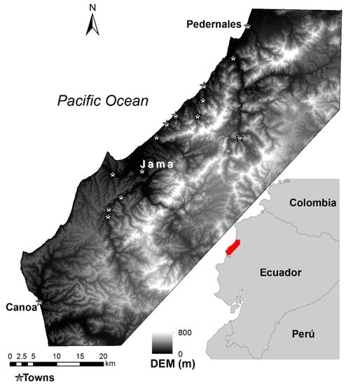
Figure 1.
Location of the study area.
The major land cover types of the study area include pasture for cattle ranching, patches of relatively well-preserved forests (old-growth forest), secondary forest, and agriculture, including forestry plantations. Remaining forest patches likely experienced selective logging and other human impacts, but many are well preserved, partially because of landowner decisions. Secondary forests are mostly the result of pasture abandonment due to a change of livelihood or occasionally pasture-fallow cycles following years of intensive ranching. Most of the study area follows the patterns of deforestation for cattle ranching practiced from the 1950s and 1960s until the 1980s or early 1990s, when banned exports due to foot and mouth disease complicated the livestock market [35,41]. Most secondary forest areas, therefore, are reported to be around 20 years old. Cattle pasture is the dominant land cover type, planted with exotic grasses. Forestry plantations are mostly teak (Tectona grandis) monocultures but other timber species such as balsa (Ochroma pyramidale) have been also recorded. Plantations developed as a result of combined market incentives and low livestock prices that attracted some big cattle ranchers who were able to wait long periods of time until harvest to receive financial returns.
We selected this study region because of its importance for biodiversity conservation. The geographic extent of different forest types is unknown and changes in land cover have not been assessed. At least partially, this is due to the difficulty of correctly classifying spectrally similar land cover types, such as different forest types and even pastureland against forest without a fully closed canopy. The limited availability of cloud-free satellite remote sensing data and lack of ground inventories of some land cover types (e.g., secondary forests) represent additional challenges for land cover change analyses.
2.2. Satellite Image Collection and Preparation
Remotely sensed imagery for classification and land cover change analysis included Landsat 5 (Thematic mapper [TM]), Landsat 7 (Enhanced Thematic Mapper [ETM+]) and Landsat 8 (Operational Land Imager [OLI]) images. We downloaded images from the United States Geological Survey (USGS) at <www.glovis.com>. Atmospheric correction was applied to all images to reduce atmospheric effects. Then, images were converted to radiance values and then into surface reflectance values using minimum dark object subtraction. Gain, offset and sun elevation data angles were obtained from the USGS GeoTIFF metadata. To correct for striping in ETM images because of the line drop problems inherent to Landsat 7 data, we performed gap-filling using focal analysis in ERDAS Imagine [42]. This procedure did not substantially change the original image because most of the study area was in portions of the image not affected by striping.
No images free of cloud and associated cloud shadow were available for classification analysis for the 2013‒15 period when training data were collected. Because we specifically wanted to account for seasonality, a November ETM+ image of 2013 and a March OLI image of 2015 were selected as having the best quality images available for the dry and rainy seasons. These primary images had between 10% (ETM image—dry season) and 20% (OLI image—wet season) of the study area covered by clouds. To circumvent this problem, we masked cloud and cloud shadow from primary images and used cloud-free sections of auxiliary images to substitute masked sections. One additional image for the dry season and two additional images for the wet season were selected as auxiliary images. Auxiliary images were of the same season and year of the primary image. To ensure that primary and auxiliary images did not differ spectrally from each other, we compared the spectral signatures of cloud-free sections of all images to be mosaicked. The object-based cloud and cloud shadow detection algorithm Fmask 3.2 version was applied to identify cloud and cloud shadow pixels in all images [43,44]. Fmask successfully identified cloud shadows, but occasionally mistook clouds with sandy beaches and built-up areas. In these cases, we manually built cloud masks based on unsupervised classifications and used these masks for cloud extraction. The combination of Fmask and cloud masks derived from unsupervised classifications resulted in the best detection possible to remove cloud and cloud shadow from all images. For image composition, the primary images from each season were selected as the reference images. No-data values from cloud and cloud-shadow removed pixels in reference images were replaced with available data from auxiliary images to obtain one image for each season.
The same procedure was followed for the 1990 image that was used for land cover change analysis. This was the only image with some cloud-free areas, which allowed for a classification of the 1990s, where most secondary succession is estimated to have started [35,39]. Areas of cloud and cloud shadow remained with no data. Image preparation was conducted in ENVI and ERDAS Imagine. Image pre-processing steps are summarized in Figure 2 (dashed box).
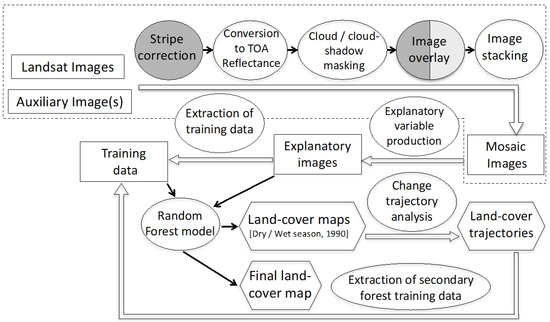
Figure 2.
Flow chart of image pre-processing and classification processing steps. Squares denote images and training data, circles image processing steps, and hexagons land cover or land cover-derived products. White indicates steps involving all Landsat images (TM, ETM and OLI), dark gray represents steps involving only ETM images, and light gray show steps involving only OLI images. The dashed box denotes image collection and preparation, areas outside the dashed box classification and change trajectory models.
2.3. Training Data Collection
We selected 947 training data pixels for image classification of areas of old-growth forests, pastures, teak plantations, water, and built-up areas. Not enough reliable information about secondary forests was available to obtain a similar number of training points. We, therefore, excluded secondary forest as a class in initial analyses, but see Section 2.6 for an approach to map secondary forests.
Old-growth forest training data were derived from a combination of surveyed plot data and available polygons of protected forests. A total of eight forest sites were inventoried during 2010 and 2012. Polygons from these areas were obtained from their owner or manually digitized. Protected forests refer to areas under a governmental payment-for-conservation scheme named Socio Bosque program [37]. Areas under Socio Bosque in the study areas were used to complement surveyed old-growth forest sites. In all obtained forest polygon sites (sampled plus Socio Bosque areas), random points were generated in ArcGIS ensuring a distance >10 pixels between them, to increase variability, and a buffer of 30 m from polygon edges, to avoid edges, to obtain a total of 233 forest training points.
Pasture training points included inventoried pasture sites along the coastal road that connects the major towns of Pedernales, Jama, and Canoa. As additional sources of information, we used freely available Quickbird images from Google Earth of the proximities of Pedernales (Figure 1). With combined field inventories and visual inspection of Google Earth images, we obtained a total of 231 pasture training points.
Teak plantation was probably the most difficult land cover type to differentiate because of the similarities between plantation and other tree-dominated land cover types and lack of any other auxiliary data. Therefore, we rely exclusively on field collected training data for teak plantations. We mapped the field plantation sites and obtained digitized plantation polygons. In all obtained plantation polygon sites, training points were generated in ArcGIS, ensuring a distance of at least two pixels between them to obtain a total of 179 plantation training points. The number of plantation training points is slightly lower compared to other land cover types, but plantations are even-age single-species stands with little variability across sites. We excluded recently planted teak in pastureland because teak trees in these immature plantations were single stems of less than 3 m tall. These young plantations exhibited high amounts of grass species, in similar or even greater coverage than in pasture areas used actively for cattle ranching. Plantations of other timber species such as pachaco (Schizolobium parahyba) or balsa (Ochroma pyramidale) were too small or immature to be included in our analyses.
To complement sampled data, a total of 154 water training-points and 150 built-up training points were generated. For the water land cover type, rivers and rice or shrimp farms close to the major towns of Jama and Pedernales were digitized and then random points in ArcGIS were generated within digitized polygons. We relied exclusively on in-land water areas, excluding the ocean, because streams and shrimp or rice fields were lighter than the ocean due to shallow water depth and the presence of sediments. At the same time, large inland water areas were spectrally distinctive enough from adjacent ground areas to be identified visually. To obtain training points of built-up areas, towns were digitized based on researchers’ local knowledge of the area, field visits, and points’ distinct spectral reflectance. These included Jama and Pedernales, the two major urban centers of the study area (Figure 1).
2.4. Explanatory Variable Data
The two mosaicked Landsat images for the wet and dry seasons produced after cloud/cloud-shadow removal and image overlay were used to calculate 46 explanatory variables. One of the greatest advantages of RF is that it is does not over fit the data because with the large number of classifying trees, there is a low generalization error [45,46]. We therefore used a large array of Landsat derived explanatory variables with the ultimate goal of producing accurate land cover maps of the study area. Explanatory variable data included most Landsat bands, including the thermal bands reported to be important in tropical dry forest land cover classifications [47]. We calculated simple ratios between bands reported to be significantly correlated with many forest stand characteristics in tropical rain forests [48], vegetation indices used in similar studies [31,32,33,34,49], and image transformations known to be associated with major changes in land cover [48]. We also calculated variance-based textural indices at a 3 × 3 window of all previous indices and of all Landsat bands. Variance-based texture at this window size was found important in characterizing forest habitats and classifying complex landscapes [50,51]. Also, a 3 × 3 window was estimated the most accurate because some land cover types were very narrow or small in area. We excluded indices derived from digital elevation models because field inspections indicated that the occurrence of most land cover types was related at a high extent to land ownership rather than to characteristics of the terrain. A complete list of all explanatory variables and their formulas is given in Table 1.

Table 1.
Predictor variables used in Random forests (RF) classifications. Variables were calculated independently for the dry and wet seasons. The last column specifies the names used to identify variables elsewhere in this manuscript. ETM = Enhanced Thematic Mapper, OLI = Operational Land Imager.
2.5. Land Cover Classification Models
We used Random Forest (RF) as a classification approach. RF is a machine learning technique that consists of tree-structured classifiers built by bootstrapped randomly selected predictors [45]. By randomization of the predictors, a large number of tree-structured classifiers are produced and aggregated producing a model that is less prone to overfitting the training data. The selection of multiple predictors increases classification accuracy because the tree-structured classifier with the best set of predictors is selected while the weaker ones are avoided. Compared to similar techniques, RF has many advantages: higher accuracy, the ability to model complex interactions among predictor variables, flexibility to perform many statistical analyses (i.e., classification and unsupervised learning), and an ability to deal with missing values [45,50,52,53,54].
To assess the importance of season in land cover classifications, we built three models and created three land cover maps for comparison: a dry season map based on explanatory variables of the dry season, a wet season map based on explanatory variables of the wet season, and a combined bi-seasonal model with explanatory variables from both seasons. RF models were used to classify the study area into: forest, plantation forest, pasture, built-up areas, and water. In these first classifications, the forest class included old-growth and secondary forests.
The ModelMap package in R was used to build the RF models and create land cover maps [46,55]. ModelMap provides an interface between existing R packages including randomForest, raster and rgdal to automate and simplify model construction and map creation. Because ModelMap optimizes the parameters of RF, we kept ModelMap default values. The default for the number of predictor variables randomly sampled as candidates at each decision tree node split (parameter mtry), was the square root of the total number of predictor variables. The parameter ntree, which defines the number of decision trees constructed as part of the classifier ensemble, was kept at 500. Large values of ntree have not been found to over fit models [46,55]. In RF, out-of-bag predictors are used to construct confusion matrices to calculate overall Kappa values for each model and errors of omission and commission, and to produce an assessment of variable importance, calculated by measuring the mean decrease in accuracy if a feature is left out in building a tree.
2.6. Change Detection and Secondary Forest Mapping
To assess changes in forest cover, we performed change trajectory analyses of the ‘forest’ class derived from the 2013‒15 RF classifications and a land cover classification derived from a RF classification of the 1990 image. This image was classified into forest, pasture, built-up, and water. The plantation class was excluded because there was no historic or anecdotal record that plantations were present in 1990. For the ‘forest’ class, we relied on the same training points used in the 2013‒15 land cover classifications. These sites are estimated to be well-preserved forests and therefore expected to represent forest sites from 1990 too. Training points for the pasture land cover class were obtained from those recorded in 2014. To maximize the likelihood that selected pasture areas were pasture in 1990 we relied more on areas in close proximity to roads and human settlements and whose spectral signatures in the 1990 image were close to those of the 2013‒15 wet season image. Training points for the built-up land cover class were obtained by a combination of visual inspection of images and geographic locations of areas in the towns of Pedernales and Jama. The water land cover class was easily identified visually because of its contrasting spectral signature.
After obtaining a 1990 land cover map with the following land cover classes—forest, pasture, water, and built-up—the last three were merged into a single non-forest class. This land cover map was used to perform change trajectories with the 2013‒15 dry, wet, and bi-seasonal land cover maps. Areas that transitioned from non-forest in 1990 to forest in 2013‒15 estimate areas of secondary forest. Areas that transitioned from forest to other land cover types highlight deforestation patterns. Transitions from forest and non-forest to plantation help clarify the geographic extent of plantations as it is expected that current plantations developed in previous pastureland.
To evaluate the performance of RF in classifying old-growth forest, secondary forest, and plantation forest, we used areas identified as secondary forests by trajectory analyses to obtain secondary forest training data and re-run the original RF models with secondary forest as a class. We selected only areas identified as secondary forest in all three-trajectory land cover maps and of at least 9000 m2 to increase the likelihood of selecting true secondary sites. In these areas, a total of 235 secondary forest training points were obtained and added to the original RF training data within a buffer of 30 m to avoid potential edges. The three RF models (dry, wet, and bi-seasonal) were run again with the following land cover categories: old-growth forest, secondary forest, plantation forest, pasture, water, and built-up areas. The steps to generate land cover and change trajectory maps from Landsat images and training data using RF is summarized in Figure 2 (outside the dashed box).
3. Results
3.1. Classification Results
The bi-seasonal RF model, which included metrics from the dry and wet seasons, resulted in the highest out-of-bag accuracy at 95.3% (Kappa = 0.94). Using metrics from the dry season alone achieved a slightly lower accuracy of 94.6% (Kappa = 0.93) while using metrics of just the wet season resulted in an accuracy of 92.8% (Kappa = 0.91; Table 2a). Training data from the forest, built-up, and water land cover classes were more accurately classified in the bi-seasonal model (higher producer accuracy). Plantation forest training data were equally well classified in both the dry and bi-seasonal models, while pasture training data were classified slightly better in the dry season model. User’s accuracy for all land cover types was also higher in the bi-seasonal model, with the exception of pasture, which had a higher value in the dry season model. These numbers indicate that the bi-seasonal model had a better performance for most land cover types, but a slightly greater tendency to misclassify pasture data. Classification and misclassification details can be appreciated in greater detail in the confusion matrices of the training data (Table 2b). A slightly higher confusion between pasture and forest training data occurs in the bi-seasonal model compared to the dry season model. Difficulties in differentiating forest from pasture are higher in the wet season model compared to the other two models, suggesting a lower performance of this model to classify forest. Regarding the plantation forest class, numbers are very similar across models, but misclassification in the bi-seasonal model occurs almost exclusively with the pasture class while plantation forest data tend to be mistaken more with forest data in the dry and wet season models. Details of the confusion matrices for all land cover types in all three models are summarized in Table 2b.
Table 2.
Overall producer’s and user’s accuracies (a) and confusion matrices (b) for the three Random Forest (RF) models.
The classification maps show that, while differences in out-of-bag accuracies between the three models are small, the resulting maps exhibit some important differences. Percent forest cover in the study area according to our models ranges between 38% (dry season model), 41% (bi-seasonal model) and 45% (wet season model). Variation was expected due to the seasonality of tropical dry forests and the fact that different sections of the images were masked out in each model, but some is related to differences in the models. In general, forest areas in the study area occur mostly along the coast, with two of the biggest forest patches sharing a coast line. The dry and bi-seasonal models resemble what could be expected of the forest based on knowledge of some areas (Figure 3A,C). The wet season model underperforms in classifying areas expected to be forest, especially in the southern portion of the landscape where many of these areas are mistakenly classified as plantation forest (Figure 3B inset map). The wet season cover map suggests 10% plantation coverage in the landscape. This value is 6% and 7%, respectively, in the dry and bi-seasonal models. The dry and bi-seasonal models differ mostly on where plantation occurs. In the dry season cover map, plantation forests are scattered through the landscape while in the bi-seasonal map, these are more concentrated in the central portion of the landscape (Figure 3A,C). It is challenging to assess whether the dry or the bi-seasonal model does better at identifying areas of plantation forests. Some areas in the southeastern portion of the landscape (Figure 3A,C inset maps), classified as plantation and pasture in the bi-seasonal model, are classified as built-up in the dry season model. This could indicate an overall better performance of the bi-seasonal model as these areas likely correspond to water-stressed pasture or exposed soil in the dry season model rather than to big human settlements. Moreover, differences in the extent of plantation forest result from mostly misclassified forest in the dry season model, but from misclassified pasture in the bi-seasonal model. Therefore, the bi-seasonal model better maps forest types because of a clearer distinction between introduced and natural forest.
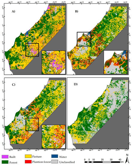
Figure 3.
Random Forests (RF) land cover classification maps. (A) RF using predictor variables from the dry season. (B) RF using predictor variables from the wet season. (C) RF using predictor variables from the dry and wet seasons. (D) 1990 RF classification. Inset maps show locations of important transitions discussed in the text.
3.2. Importance Measure of Variables
The relative importance of the most used predictors in each of the three RF classification models highlight variables of critical importance to classifying the studied tropical dry forest landscape (Figure 4). The wet and dry season models share top predictors to a good extent. The thermal band was the most important predictor in both models. Although the thermal band has not been used extensively in land cover classifications, its importance in tropical dry forest landscapes has been previously reported [47]. Other variables that contributed to our classification models (with a mean decrease of accuracy >20%) include simple ratios that utilize the red, near infrared, and short-wave infrared Landsat bands, which are sensitive to differences in forest stand parameters (e.g., biomass) [48]. The ratio between the short-wave infrared and the red bands was the second top predictor in the dry season model and it was among the top predictors in the wet season model. PCA3 was important in both models while NDWI and the blue and red bands contributed significantly to the wet season model. No textural indices were significantly utilized in the dry or the wet season models (Figure 4a,b). In the bi-seasonal model, out of the 30 predictors used in the model, 15 were from the dry season and 15 from the wet season, and the most important ones were also those found important in the single season models. It was expected that strong predictors from the dry and wet season models were going to be important in the bi-seasonal model because they represent similar data but from different seasons. However, that an equal number of predictors from each season was used and that in many cases the same predictor from each season was used indicates that differences due to seasonality are complementary for classification. In the bi-seasonal model, no variable had a mean decrease of accuracy of more than 24% and accuracy values decreased more steadily, suggesting that the absence of top predictors would be less critical than in the other two models (Figure 4c).
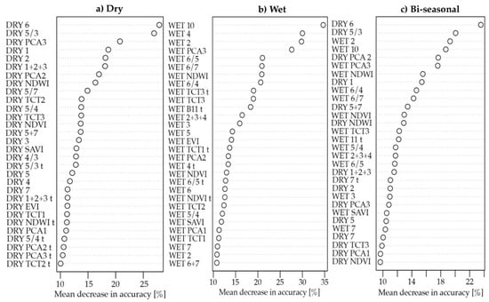
Figure 4.
Variable importance measure for the (a) dry, (b) wet, and (c) bi-seasonal RF models estimated by mean decrease accuracy if a feature were left out in building a decision tree. For acronyms and formula details of predictor variables, see Table 1.
3.3. Land Cover Change
Cloud cover on the northern part of the 1990 and on sections of the 2013‒15 cover maps allows mostly general characterizations of land cover change. Accuracy values of the 1990 RF model (Out-of-bag accuracy = 99.1%; Kappa = 0.98) provide high confidence in the 1990 cover map to identify trajectories that highlight changes in forest cover in the study area. In the 1990 RF cover map, about 61% of the analyzed pixels were classified as forest while 39% as non-forest (Figure 3D). In the three 1990–2015 trajectory maps, areas classified as forest in 1990 that remained as forest in 2013‒15 account for about 29% of the study area and correspond to old-growth forests. Old-growth forest percent values are relatively constant in all three 1990–2015 trajectory maps (Figure 5). Deforestation values over the last 25 years, or pixels that transitioned from forest in 1990 to non-forest in 2013‒15, vary more depending on the 2013‒15 cover map used. The 2013‒15 dry season cover map has the lowest cloud cover and allows for greater appreciation of deforestation patterns. The 1990–2015 (dry season) trajectory map indicates that 30% of the landscape, or half of the 1990 forest areas, were cleared during the 25-year study period (Figure 5A). This value is lower in trajectory maps involving the bi-seasonal (27%) and the wet season (23%) cover maps because of classification differences in our 2013‒15 models but also because of fewer cloud free areas in these maps (Figure 5B,C). Deforestation in the landscape occurred mostly inland in areas close to a network of primary and secondary roads in the southern portion of the landscape. It was not possible to analyze land cover change in detail in the northern portion of the landscape, but fewer roads are found in that section and we know based on the 2013‒15 cover maps that these areas are more forested. An important proportion of the areas adjacent to the coast remained forested, many of them in direct adjacency to the primary road that crosses the landscape from north to south along the coastline (Figure 5A, inset map).
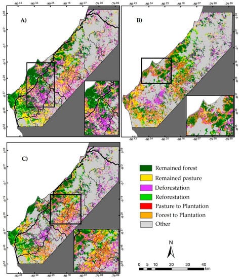
Figure 5.
Change trajectory maps between: (A) 1990 and 2013‒15 dry season, (B) 1990 and 2013‒15 wet season, and (C) 1990 and 2013‒15 bi-seasonal. Other includes areas of cloud, cloud shadows, and other transitions. Inset maps show locations of important transitions discussed in the text. Lines indicate primary, secondary, and tertiary roads.
Land cover trajectories from 1990 pastures to 2013‒15 forests serve to identify areas of forest re-growth or secondary forests. The trajectory maps between the 1990 and the 2013‒15 dry and bi-seasonal cover maps exhibit similar numbers in regards to the extent of secondary forest. According to these maps, about 12% of the landscape is secondary forest. This percent is higher (16%) in the wet season transition map. Forest regeneration occurred mostly in small patches, almost exclusively adjacent to big forest patches (Figure 3A,C).
Land cover trajectories that resulted in plantation forest in 2013‒15 are important to explain differences in plantation forest percent cover and extent between the 2013‒15 cover maps. Plantations are reported to occur in areas that were formerly pasture. It is expected therefore that most plantation forest areas in 2013‒15 were pasture in 1990. Pasture in 1990 that transitioned to plantation forest in 2013‒15 accounts for 3% of the landscape in the 1990–2015 (dry season) trajectory map, 7% in the 1990–2015 (wet season) trajectory map, and 6% in the 1990–2015 (bi-seasonal) trajectory map. Areas that transitioned from forest in 1990 to plantation in 2013‒15 do not follow reported land use trajectories. It is possible that some of these areas correspond to forests cleared later in the 1990s that grew to full canopy-covered plantations, but areas where forest to plantation forest is the dominant transition might indicate areas were our models are performing poorly. That is the case of plantation areas by the coastline in the 1990–2015 (wet season) trajectory map (Figure 3B, inset map) and areas in the central portion of the landscape in the 1990–2015 (bi-seasonal) trajectory map (Figure 3C, inset map).
3.4. Secondary Forest Mapping Using Random Forests
The addition of secondary forest as a class reduced accuracy in all RF classification models. The bi-seasonal model had the highest out-of-bag accuracy (87.9%; Kappa = 0.85) followed this time by the wet season model (overall accuracy = 85.8%; Kappa = 0.82) and the dry season model (overall accuracy = 82.9%; Kappa = 0.79). Producer’s and user’s accuracy was the highest in the bi-seasonal model for all six-analyzed land cover types, with the exception of pasture user’s accuracy, which was higher in the dry season model (Table 3a). Lower model accuracies resulted mostly from difficulties differentiating secondary from old-growth forests. In the bi-seasonal model, 69% of the training data of old-growth forest and 80% of the secondary forest training data were correctly classified. These values are significant considering the difficulties of differentiating old-growth from secondary forests using Landsat data. Classification and misclassification of the training data from the plantation forest, built-up, and water land cover classes resembles very closely that of the previous models (Table 3b).
Table 3.
Overall producer’s and user’s accuracies (a) and confusion matrices (b) for the three Random Forests (RF) models with secondary forest data derived from change trajectories included.
The newly produced cover maps resemble the previous ones closely but with details about which forest areas are old-growth and which are secondary. Because the bi-seasonal model performed better, for simplicity and greater appreciation of details, just the bi-seasonal cover map is presented in Figure 6 as the final cover map of this research, but data from all three are discussed. The produced maps indicate that percent old-growth forest cover in the study area ranges between 17% (Bi-seasonal model), 16% (wet season model) and 15% (dry season model). Old-growth forests are concentrated to the central portion of the landscape and to scattered areas within big forest patches. The concentration of old-growth forest pixels is particularly high in two areas that correspond to two known reserves: Lalo Loor and Jama Coaque. That areas within these reserves were found to be old-growth forest serves as independent validation of the produced cover map (Figure 6, inset map b).
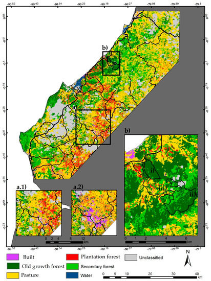
Figure 6.
Final Random Forests (RF) land cover classification map using predictor variables from the dry and wet seasons. Inset map (a) shows areas of conflicting classification between the dry season (a.1) and bi-seasonal (a.2) models. Inset map (b) show the location of (i) Lalo Loor reserve, (ii) Jama Coaque reserve, iii) Jama Coaque areas of reforestation, native tree planting and pasture. Lines indicate primary, secondary, and tertiary roads.
Secondary forest apparently accounts for larger portions of areas previously identified as forest, with cover varying between 28% (wet season model) and 25% (dry and bi-seasonal models). Percent cover of old-growth and secondary forest from the RF models is different than that estimated by land cover change between the 1990 and 2013‒15 images (29% old-growth forest, ~12% secondary forest). These differences should be interpreted considering that an important number of forests likely experienced various degrees of human interventions and degradation since the 1990s and could resemble structurally more secondary than old-growth forests. The only external validation available for secondary forests is records of 12 60 × 60 m plots used for floristic composition analyses. Seven of the 12 inventoried secondary forest plots have at least some secondary forest pixels in them, two have only old-growth forest pixels, two only pasture pixels and one old-growth and plantation forest pixels. Additionally, a small section of the Jama Coaque reserve known as “finca” dedicated to reforestation and native tree planting in areas formerly covered by pasture and agroforests were classified as mostly pasture and secondary forest (Figure 6, inset map b).
Differences in plantation forest cover between our models were reduced by incorporating the secondary forest class. The new models found that plantation forest accounts for between 10% (wet season model) and 8% (dry and bi-seasonal models) of the landscape. We attempted to reduce discrepancies in the interior of the landscape by adding additional plantation training data, but differences persisted (Figure 6, inset map a). Finally, percent pasture coverage was 47% (bi-seasonal model), 46% (dry season model), and 44% (wet season model), slightly lower than coverage found in the RF models with no secondary forest data.
The relative importance of the 30 most important predictors in the RF with secondary forest data resembles closely that of the previous models. The thermal band as well as PCA3, single bands, and indices sensitive to differences in forest stand parameters were important [48]. The only significant difference is that the bi-seasonal model used more variables from the wet season (17) than from the dry season (13) compared to the equal number of variables from each season used in RF with no secondary forest data (Figure 7).
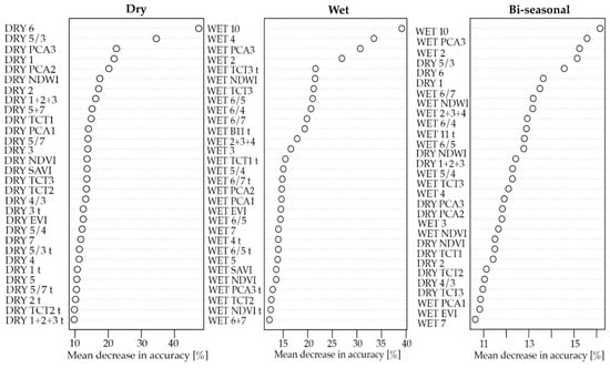
Figure 7.
Variable importance measure for RF models with secondary forest data: (a) dry, (b) wet, and (c) bi-seasonal. Importance is estimated by mean decrease accuracy if a feature were left out in building a decision tree. For acronyms and formula details of predictor variables, see Table 1.
4. Discussion
4.1. Forest Type Classification
Using bi-seasonal Landsat data to map old-growth, secondary, and plantation forest resulted in overall higher out-of-bag accuracy than when using single season data. This finding is in agreement with studies conducted in other tropical vegetation types [33,34]. In the humid tropics, adding multi-temporal data increased classification accuracy in landscapes composed of forest types more similar than the ones of this research. However, it was stressed that efforts related to including multi-temporal data are worth undertaking depending on classification objectives and contingent to having high quality images [33]. In our study, when old-growth and secondary forest were grouped in a single class, classification accuracy using dry season data resulted in similar values to that obtained with bi-seasonal data while accuracy values were lower when only wet season data was used. The importance of multi-temporal data became more critical when our analyses included three different forest types: plantation, old-growth, and secondary. Differences between model accuracies increased and the classification based on wet season data only became more reliable than the one based on dry season data only. As the number of forest classes increases (e.g., by incorporating agroforests or other types of plantations), we expect bi-seasonal data to become even more important. The number of forest classes should therefore guide the use of single or bi-seasonal Landsat data in classification.
Differences between the derived land cover maps of our models, especially in regards to the coverage of the plantation forest class, serve to highlight some of the limitations of RF. Plantation forest training data were consistently classified with over 90% accuracy in all of our models, but the land cover maps produced show some significant discrepancies, especially in areas of the landscape where training data were not possible to collect. The extent of teak plantation forest cover in the study is low, and it is possible that other plantation types of even lower canopy coverage (e.g., balsa, cacao, citrus, papaya plantations) could be mistaken with teak plantations. Also, RF assumes training data are spatially independent from each other, which helps explain discrepancies in our land cover maps in areas where field sampling was not possible. We recommend therefore to examine plantation coverage in terms of percent landscape coverage and plantation type. At present, plantation forest covers less than 10% of the study area, and some of the areas identified as teak plantation could in fact be other plantation types. RF proved to be a valid tool to accurately classify plantation forest, but mapping its coverage could be further improved by geographically expanding the collection of training data.
4.2. Variable Importance
The use of Landsat-derived predictors in our models provides details about which variables are important to classify elements of tropical dry forests, a result previously reported only for humid tropics. Similar to that reported for humid tropical forest landscapes, we found that the blue and red wavelength bands contributed substantially to separate forest types [34]. The red, near infrared, and short-wave infrared were also important, but we found they served better in the form of simple ratios than as individual bands [48,49]. These bands and indices are sensitive to stand parameters and photosynthetic activity and therefore important to forest classification in general [48] The thermal band is not listed as an important variable in RF classifications of other forest types. We found, however, that the thermal band was the most important predictor in our models. Only one study suggested that the thermal band could significantly aid classification, especially in tropical dry forests, because forest age and successional stages are evident from temperature surfaces [47]. These reported forest characteristics, where thermal data are important, are in agreement with the structural differences in the forest types analyzed in this research. We did not reduce the number of variables in our models because the RF technique does not require this to run efficiently and because we intended to provide as complete information as possible on the utility of Landsat data in classifying tropical dry forests. The selection of the RF methodology for use with remotely sensed data is ideal due to the random selection of variables that allow the modeling of complex interactions (e.g., correlation) of predictors without overfitting the model. Given that the ultimate goal of a classification approach is to produce a reliable land cover map, we advise using RF classification approaches when large numbers of potential predictors are available, some of which may be correlated and numerous. In such instances the RF approach will outperform most traditional classification techniques and be more reliable and robust [45,52,54].
4.3. Tropical Dry Forests in Coastal Ecuador
The produced land cover maps and the land cover change analysis provide information about changes in forest cover in the studied landscape. We found that 50% of the forest areas present in 1990 were cleared during the 25-year study period, agreeing with numerous reports that list tropical dry forest in general, and this study area, in particular, as critically endangered [16,17,18,19]. We expected to find deforestation associated with areas of high road density, but we did not expect to find many of the remaining forest patches along the coast and adjacent to major roads. The entire landscape is privately owned, so we believe these patterns reflect to a good extent landowners’ decisions on how to manage their land. The finding that most of the forest patches in the landscape were secondary forest while old-growth forest was almost entirely restricted to reserves was surprising. We anticipated that areas inside reserves would be classified as old-growth forest, but we expected other large patches outside reserves to also be classified as old-growth forest. We acknowledge that our approach at obtaining secondary forest training data could increase old-growth and secondary forest misclassification. However, at least at a landscape level, we believe our results reflect the state of forests in the area. Selective logging and continuous perturbations related to the presence of cattle are known to occur in the area [17,22], negatively impacting forest remnants. Despite the privatized nature of the landscape, it is likely that illegal logging occurs as well. Reports of reforestation in the area exist, but we believe the vast majority of the areas classified in our models as secondary forest correspond to forest at different stages of degradation, such that they structurally resemble secondary forest more than old-growth forest.
Tropical dry forests are one of the most threatened ecosystems due to their limited remaining extent and the high threat from human activities [16,17]. In the Neotropics, documenting their distribution, extent, and degree of fragmentation is still considered a research priority [17]. In Ecuador, very few studies have quantitatively estimated land cover and land cover change in dry forest areas. Our results represent one of the first assessments, despite all the challenges associated with conducting remote sensing analysis in this area and the limitations of our findings. The coast of Ecuador is an area where massive changes in land cover have been historically reported [35]. Our finding that 50% of forest present in 1990 in the study areas was cleared, provides a conservative estimate for other areas as higher deforestation is expected in areas where human activities are more intense. Tropical dry forests are also poorly represented in the national network of protected areas and is a local conservation priority as a result [36,37]. The forest classification provided in this study could help target conservation efforts and support those currently existing.
5. Conclusions
This study aimed to differentiate forest types and understand changes in their coverage in a highly threatened tropical dry forest in Ecuador. Based on our results, we can draw two general conclusions: (1) The studied landscape has lost approximately half of the forest present in 1990. Remaining old-growth forest is mostly restricted to existing conservation areas. We believe the forests classified as secondary include forest re-growth but also degraded forest structurally resembling secondary forest. These forests account for the majority of forest patches outside conservation areas. Plantation forest accounts for over 10% of the landscape area, but this result should be interpreted cautiously considering that only mature plantation forests were included in this study. (2) Using a RF classifier with spectral metrics derived from Landsat provided reliable classification results. We discriminated natural from planted forest with an overall accuracy of 95% and old-growth, secondary, and plantation forest with an overall accuracy of 88%. Including bi-seasonal data resulted in higher accuracy in all models, and having seasonal data was even more important when classifying three forest classes. As the number of land cover types, especially those dominated by vegetation, or the extent of current forest types increases, the importance of bi-seasonal data in classification is expected to increase.
Author Contributions
X.H. recorded and analyzed the data, and wrote this paper. X.H. and J.S. designed this research and discussed results.
Funding
This research received no external funding.
Acknowledgments
This research was supported by the Secretaria Nacional de Ciencia y Tecnología, Ecuador (SENESCYT) and the Tropical Conservation and Development Program (TCD) at the University of Florida. The Ceiba Foundation for Tropical Conservation provided extensive logistic support to conduct fieldwork in the area. The Jama Cuaque reserve provided information on their premises. The Ministry of Environment of Ecuador provided information on areas under the Socio Bosque conservation program and granted permission for this study. The people of Tabuga are specially thanked for their assistance in the field, for allowing us to conduct fieldwork in their properties, and for sharing their knowledge about the area. Bette Loiselle provided comments and constructive criticism. Craig Noles assisted with English editing. Publication of this article was funded in part by the University of Florida Open Access Publishing Fund.
Conflicts of Interest
The authors declare no conflict of interest.
References
- Hansen, M.C.; Potapov, P.V.; Moore, R.; Hancher, M.; Turubanova, S.A.; Tyukavina, A.; Thau, D.; Stehman, S.V.; Goetz, S.J.; Loveland, T.R.; et al. High-Resolution Global Maps of 21st-Century Forest Cover Change. Science 2013, 342, 850–853. [Google Scholar] [CrossRef] [PubMed]
- Food and Agriculture Organization of the United Nations. Global Forest Resources Assessment 2015: How Are the World’s Forests Changing? Food and Agriculture Organization of the United Nations: Rome, Italy, 2015; ISBN 978-92-5-108821-0. [Google Scholar]
- Foley, J.A. Global Consequences of Land Use. Science 2005, 309, 570–574. [Google Scholar] [CrossRef] [PubMed]
- Riitters, K.; Wickham, J.; Costanza, J.K.; Vogt, P. A global evaluation of forest interior area dynamics using tree cover data from 2000 to 2012. Landsc. Ecol. 2016, 31, 137–148. [Google Scholar] [CrossRef]
- Chazdon, R.L.; Peres, C.A.; Dent, D.; Sheil, D.; Lugo, A.E.; Lamb, D.; Stork, N.E.; Miller, S.E. The Potential for Species Conservation in Tropical Secondary Forests. Conserv. Biol. 2009, 23, 1406–1417. [Google Scholar] [CrossRef] [PubMed]
- Sala, O.E.; Stuart Chapin, F., III; Armesto, J.J.; Berlow, E.; Bloomfield, J.; Dirzo, R.; Huber-Sanwald, E.; Huenneke, L.F.; Jackson, R.B.; et al. Global Biodiversity Scenarios for the Year 2100. Science 2000, 287, 1770–1774. [Google Scholar] [CrossRef] [PubMed]
- Lambin, E.F.; Geist, H.J.; Lepers, E. Dynamics of Land-Use and Land-Cover Change in Tropical Regions. Annu. Rev. Environ. Resour. 2003, 28, 205–241. [Google Scholar] [CrossRef]
- Turner, B.L.; Lambin, E.F.; Reenberg, A. The emergence of land change science for global environmental change and sustainability. Proc. Natl. Acad. Sci. USA 2007, 104, 20666–20671. [Google Scholar] [CrossRef]
- Achard, F.; Stibig, H.-J.; Eva, H.D.; Lindquist, E.J.; Bouvet, A.; Arino, O.; Mayaux, P. Estimating tropical deforestation from Earth observation data. Carbon Manag. 2010, 1, 271–287. [Google Scholar] [CrossRef]
- Gibbs, H.K.; Ruesch, A.S.; Achard, F.; Clayton, M.K.; Holmgren, P.; Ramankutty, N.; Foley, J.A. Tropical forests were the primary sources of new agricultural land in the 1980s and 1990s. Proc. Natl. Acad. Sci. USA 2010, 107, 16732–16737. [Google Scholar] [CrossRef]
- DeFries, R.; Achard, F.; Brown, S.; Herold, M.; Murdiyarso, D.; Schlamadinger, B.; de Souza, C. Earth observations for estimating greenhouse gas emissions from deforestation in developing countries. Environ. Sci. Policy 2007, 10, 385–394. [Google Scholar] [CrossRef]
- Achard, F. Determination of Deforestation Rates of the World’s Humid Tropical Forests. Science 2002, 297, 999–1002. [Google Scholar] [CrossRef]
- Asner, G.P.; Rudel, T.K.; Aide, T.M.; Defries, R.; Emerson, R. A Contemporary Assessment of Change in Humid Tropical Forests. Conserv. Biol. 2009, 23, 1386–1395. [Google Scholar] [CrossRef] [PubMed]
- Asner, G.P.; Knapp, D.E.; Broadbent, E.N.; Oliveira, P.J.; Keller, M.; Silva, J.N. Selective logging in the Brazilian Amazon. Science 2005, 310, 480–482. [Google Scholar] [CrossRef] [PubMed]
- Herold, M.; Mayaux, P.; Woodcock, C.E.; Baccini, A.; Schmullius, C. Some challenges in global land cover mapping: An assessment of agreement and accuracy in existing 1 km datasets. Remote Sens. Environ. 2008, 112, 2538–2556. [Google Scholar] [CrossRef]
- Janzen, D.H. Management of Habitat Fragments in a Tropical Dry Forest: Growth. Ann. Mo. Bot. Gard. 1988, 75, 105–116. [Google Scholar] [CrossRef]
- Sanchez-Azofeifa, G.A.; Quesada, M.; Rodriguez, J.P.; Nassar, J.M.; Stoner, K.E.; Castillo, A.; Garvin, T.; Zent, E.L.; Calvo-Alvarado, J.C.; Kalacska, M.E.R.; et al. Research Priorities for Neotropical Dry Forests1. Biotropica 2005, 37, 477–485. [Google Scholar] [CrossRef]
- Miles, L.; Newton, A.C.; DeFries, R.S.; Ravilious, C.; May, I.; Blyth, S.; Kapos, V.; Gordon, J.E. A global overview of the conservation status of tropical dry forests. J. Biogeogr. 2006, 33, 491–505. [Google Scholar] [CrossRef]
- Myers, N.; Mittermeier, R.A.; Mittermeier, C.G.; Da Fonseca, G.A.; Kent, J. Biodiversity hotspots for conservation priorities. Nature 2000, 403, 853–858. [Google Scholar] [CrossRef]
- Mittermeier, R.A.; Turner, W.R.; Larsen, F.W.; Brooks, T.M.; Gascon, C. Global Biodiversity Conservation: The Critical Role of Hotspots. In Biodiversity Hotspots; Zachos, F.E., Habel, J.C., Eds.; Springer: Berlin/Heidelberg, Germany, 2011; pp. 3–22. ISBN 978-3-642-20991-8. [Google Scholar]
- Brooks, T.M.; Mittermeier, R.A.; Mittermeier, C.G.; Da Fonseca, G.A.; Rylands, A.B.; Konstant, W.R.; Flick, P.; Pilgrim, J.; Oldfield, S.; Magin, G.; et al. Habitat Loss and Extinction in the Hotspots of Biodiversity. Conserv. Biol. 2002, 16, 909–923. [Google Scholar] [CrossRef]
- Lyons-Galante, H.R.; Haro-Carrión, X. Effect of distance from edge on exotic grass abundance in tropical dry forests bordering pastures in Ecuador. J. Trop. Ecol. 2017, 33, 170–173. [Google Scholar] [CrossRef]
- Chazdon, R.L. Beyond deforestation: Restoring forests and ecosystem services on degraded lands. Science 2008, 320, 1458–1460. [Google Scholar] [CrossRef] [PubMed]
- Chazdon, R.L.; Letcher, S.G.; van Breugel, M.; Martinez-Ramos, M.; Bongers, F.; Finegan, B. Rates of change in tree communities of secondary Neotropical forests following major disturbances. Philos. Trans. R. Soc. B Biol. Sci. 2007, 362, 273–289. [Google Scholar] [CrossRef] [PubMed]
- Tropek, R.; Sedláček, O.; Beck, J.; Keil, P.; Musilova, Z.; Šímova, I.; Storch, D. Comment on “High-resolution global maps of 21st-century forest cover change”. Science 2014, 344, 981. [Google Scholar] [CrossRef] [PubMed]
- Bremer, L.L.; Farley, K.A. Does plantation forestry restore biodiversity or create green deserts? A synthesis of the effects of land-use transitions on plant species richness. Biodivers. Conserv. 2010, 19, 3893–3915. [Google Scholar] [CrossRef]
- Brockerhoff, E.G.; Jactel, H.; Parrotta, J.A.; Quine, C.P.; Sayer, J. Plantation forests and biodiversity: Oxymoron or opportunity? Biodivers. Conserv. 2008, 17, 925–951. [Google Scholar] [CrossRef]
- Lu, D.; Weng, Q. A survey of image classification methods and techniques for improving classification performance. Int. J. Remote Sens. 2007, 28, 823–870. [Google Scholar] [CrossRef]
- Immitzer, M.; Atzberger, C.; Koukal, T. Tree Species Classification with Random Forest Using Very High Spatial Resolution 8-Band WorldView-2 Satellite Data. Remote Sens. 2012, 4, 2661–2693. [Google Scholar] [CrossRef]
- Senf, C.; Pflugmacher, D.; van der Linden, S.; Hostert, P. Mapping Rubber Plantations and Natural Forests in Xishuangbanna (Southwest China) Using Multi-Spectral Phenological Metrics from MODIS Time Series. Remote Sens. 2013, 5, 2795–2812. [Google Scholar] [CrossRef]
- Grinand, C.; Rakotomalala, F.; Gond, V.; Vaudry, R.; Bernoux, M.; Vieilledent, G. Estimating deforestation in tropical humid and dry forests in Madagascar from 2000 to 2010 using multi-date Landsat satellite images and the random forests classifier. Remote Sens. Environ. 2013, 139, 68–80. [Google Scholar] [CrossRef]
- Connette, G.; Oswald, P.; Songer, M.; Leimgruber, P. Mapping Distinct Forest Types Improves Overall Forest Identification Based on Multi-Spectral Landsat Imagery for Myanmar’s Tanintharyi Region. Remote Sens. 2016, 8, 882. [Google Scholar] [CrossRef]
- Fagan, M.; DeFries, R.; Sesnie, S.; Arroyo-Mora, J.; Soto, C.; Singh, A.; Townsend, P.; Chazdon, R. Mapping Species Composition of Forests and Tree Plantations in Northeastern Costa Rica with an Integration of Hyperspectral and Multitemporal Landsat Imagery. Remote Sens. 2015, 7, 5660–5696. [Google Scholar] [CrossRef]
- Sesnie, S.E.; Finegan, B.; Gessler, P.E.; Thessler, S.; Ramos Bendana, Z.; Smith, A.M.S. The multispectral separability of Costa Rican rainforest types with support vector machines and Random Forest decision trees. Int. J. Remote Sens. 2010, 31, 2885–2909. [Google Scholar] [CrossRef]
- Dodson, C.H.; Gentry, A.H. Biological Extinction in Western Ecuador. Ann. Mo. Bot. Gard. 1991, 78, 273–295. [Google Scholar] [CrossRef]
- Cuesta-Camacho, F.; Peralvo, M.F.; Ganzenmüller, A.; Sáenz, M.; Novoa, J.; Riofrío, G.; Beltrán, K. Identificación de Vacíos de Conservación para la Biodiversidad Terrestre en el Ecuador Continental; EcoCiencia, The Nature Conservancy, Conservation International, Ministerio del Ambiente del Ecuador: Quito, Ecuador, 2006. [Google Scholar]
- De Koning, F.; Aguiñaga, M.; Bravo, M.; Chiu, M.; Lascano, M.; Lozada, T.; Suarez, L. Bridging the gap between forest conservation and poverty alleviation: The Ecuadorian Socio Bosque program. Environ. Sci. Policy 2011, 14, 531–542. [Google Scholar] [CrossRef]
- Neill, D.A. Vegetación. Monogr. Syst. Bot. Mo. Bot. Gard. 1999, 75, 13–25. [Google Scholar]
- Josse, C.; Balslev, H. The composition and structure of a dry, semideciduous forest in western Ecuador. Nord. J. Bot. 1994, 14, 425–434. [Google Scholar] [CrossRef]
- Sierra, R. Traditional resource-use systems and tropical deforestation in a multi-ethnic region in North-west Ecuador. Environ. Conserv. 1999, 26, 136–145. [Google Scholar] [CrossRef]
- Rweyemamu, M.; Roeder, P.; Mackay, D.; Sumption, K.; Brownlie, J.; Leforban, Y.; Valarcher, J.-F.; Knowles, N.J.; Saraiva, V. Epidemiological Patterns of Foot-and-Mouth Disease Worldwide: Global FMD epidemiology. Transbound. Emerg. Dis. 2008, 55, 57–72. [Google Scholar] [CrossRef] [PubMed]
- Gap-Filling Landsat 7 SLC-off Single Scenes Using ERDAS Imagine 2014TM Landsat Missions. Available online: https://landsat.usgs.gov/gap-filling-landsat-7-slc-single-scenes-using-erdas-imagine-TM (accessed on 16 November 2018).
- Zhu, Z.; Woodcock, C.E. Object-based cloud and cloud shadow detection in Landsat imagery. Remote Sens. Environ. 2012, 118, 83–94. [Google Scholar] [CrossRef]
- Zhu, Z.; Wang, S.; Woodcock, C.E. Improvement and expansion of the Fmask algorithm: Cloud, cloud shadow, and snow detection for Landsats 4–7, 8, and Sentinel 2 images. Remote Sens. Environ. 2015, 159, 269–277. [Google Scholar] [CrossRef]
- Breiman, L. Random forests. Mach. Learn. 2001, 45, 5–32. [Google Scholar] [CrossRef]
- Freeman, E.A.; Moisen, G.G.; Coulston, J.W.; Wilson, B.T. Random forests and stochastic gradient boosting for predicting tree canopy cover: Comparing tuning processes and model performance. Can. J. For. Res. 2016, 46, 323–339. [Google Scholar] [CrossRef]
- Southworth, J. An assessment of Landsat TM band 6 thermal data for analysing land cover in tropical dry forest regions. Int. J. Remote Sens. 2004, 25, 689–706. [Google Scholar] [CrossRef]
- Lu, D.; Mausel, P.; Brondízio, E.; Moran, E. Relationships between forest stand parameters and LandsatTM spectral responses in the Brazilian Amazon Basin. For. Ecol. Manag. 2004, 198, 149–167. [Google Scholar] [CrossRef]
- Tuomisto, H.; Poulsen, A.D.; Ruokolainen, K.; Moran, R.C.; Quintana, C.; Celi, J.; Cañas, G. Linking floristic patterns with soild heteregeneity and satellite imagery in Ecuadorian Amazonia. Ecol. Appl. 2003, 13, 352–371. [Google Scholar] [CrossRef]
- Rodriguez-Galiano, V.; Chica-Olmo, M. Land cover change analysis of a Mediterranean area in Spain using different sources of data: Multi-seasonal Landsat images, land surface temperature, digital terrain models and texture. Appl. Geogr. 2012, 35, 208–218. [Google Scholar] [CrossRef]
- Tuttle, E.M.; Jensen, R.R.; Formica, V.A.; Gonser, R.A. Using remote sensing image texture to study habitat use patterns: A case study using the polymorphic white-throated sparrow (Zonotrichia albicollis). Glob. Ecol. Biogeogr. 2006, 15, 349–357. [Google Scholar] [CrossRef]
- Prasad, A.M.; Iverson, L.R.; Liaw, A. Newer Classification and Regression Tree Techniques: Bagging and Random Forests for Ecological Prediction. Ecosystems 2006, 9, 181–199. [Google Scholar] [CrossRef]
- Rodriguez-Galiano, V.F.; Ghimire, B.; Rogan, J.; Chica-Olmo, M.; Rigol-Sanchez, J.P. An assessment of the effectiveness of a random forest classifier for land-cover classification. ISPRS J. Photogramm. Remote Sens. 2012, 67, 93–104. [Google Scholar] [CrossRef]
- Cutler, D.R.; Edwards, T.C.; Beard, K.H.; Cutler, A.; Hess, K.T.; Gibson, J.; Lawler, J.J. Random forests for classification in ecology. Ecology 2007, 88, 2783–2792. [Google Scholar] [CrossRef]
- Freeman, E.A.; Frescino, T.S.; Moisen, G.G. ModelMap: An R Package for Model Creation and Map Production. R Package Version 2016, 4–6. [Google Scholar]


© 2018 by the authors. Licensee MDPI, Basel, Switzerland. This article is an open access article distributed under the terms and conditions of the Creative Commons Attribution (CC BY) license (http://creativecommons.org/licenses/by/4.0/).