WSF-NET: Weakly Supervised Feature-Fusion Network for Binary Segmentation in Remote Sensing Image

Abstract

Binary segmentation in remote sensing aims to obtain binary prediction mask classifying each pixel in the given image. Deep learning methods have shown outstanding performance in this task. These existing methods in fully supervised manner need massive high-quality datasets with manual pixel-level annotations. However, the annotations are generally expensive and sometimes unreliable. Recently, using only image-level annotations, weakly supervised methods have proven to be effective in natural imagery, which significantly reduce the dependence on manual fine labeling. In this paper, we review existing methods and propose a novel weakly supervised binary segmentation framework, which is capable of addressing the issue of class imbalance via a balanced binary training strategy. Besides, a weakly supervised feature-fusion network (WSF-Net) is introduced to adapt to the unique characteristics of objects in remote sensing image. The experiments were implemented on two challenging remote sensing datasets: Water dataset and Cloud dataset. Water dataset is acquired by Google Earth with a resolution of 0.5 m, and Cloud dataset is acquired by Gaofen-1 satellite with a resolution of 16 m. The results demonstrate that using only image-level annotations, our method can achieve comparable results to fully supervised methods.

1. Introduction

Binary segmentation can distinguish target objects finely to better understand remote sensing images such as optical remote sensing images [1,2,3,4,5,6,7,8] and synthetic aperture radar (SAR) images [9,10,11,12], and thus plays an important role in many areas, including land cover mapping [1,2,3,4], change detection [5], and environmental monitoring [6,7,8,9,10,11,12]. During the past few decades, many segmentation methods have been proposed, which can be divided into the following three categories: threshold-based methods [13], edge-based methods [14,15], and graph-based methods [16,17]. With the rapid development of remote sensing technology, the information of remote sensing images is growing at a high speed, which substantially increases the difficulty of characterizing the complex image. Thus, these segmentation methods are hardly applicable due to the limitations of representation power, robustness and efficiency.

Inspired by the successful application of deep learning in other computer vision areas and benefiting from the semantic information that can be learned by deep learning, state-of-the-art segmentation methods using fully convolutional neural networks (FCNs) have become the mainstream [1,2,3,4,6,8]. When a remote sensing image is accepted to the FCN model, FCN calculates pixel-wise segmentation of the image through multiple convolutional and upsampling operations. Unfortunately, those fully supervised FCNs can only achieve good performance when providing rich pixel-level labels for training. Obtaining pixel-level labels manually is time consuming, and geology expertise is generally required to accurately mark out uncertain margins such as cloud borders [18] and classify ambiguities such as desert regions and runway regions [19].

Recently, training segmentation models from weak annotations has gained more attention in computer vision area [20,21,22,23,24,25,26,27,28,29,30]. It aims to leverage weak annotations instead of pixel-level ones to train models for object segmentation. Weak annotations include image-level label [20,21,22,23,24,25], point [26], scribble [27,28], and bounding box [29,30] supervision, etc. Among them, image-level label has been widely utilized since it is the simplest form and only requires indicating whether an image contains the object of interest in training data, which is also termed as image-level annotation. Statistical results show that manually obtaining a pixel-level annotation for a remote sensing image with 512 $\times$ 512 pixels is about 164.73 s, whereas an image-level annotation only requires 1 s. To take advantage of this annotation, this paper explores the issue of weakly supervised binary segmentation in remote sensing image.

Most image-level weakly-supervised object segmentation methods in computer vision can be coarsely classified into multi-instance learning (MIL) based methods [24,25] and localization-based methods [20,21,22,23]. In MIL-based methods, each image-level label is assigned to a set of features, and then the pixel-level predictions are aggregated into losses [31]. However, it fails to consider object localization information, which is implicitly learned by an FCN [32,33,34]. Based on the development of localization, localization-based methods [20,21,22,23], which retrieve object regions for guiding the segmentation model training, have become the mainstream. However, the performance of such computer vision methods directly applied to remote sensing images is unsatisfactory, mainly due to the following reasons:

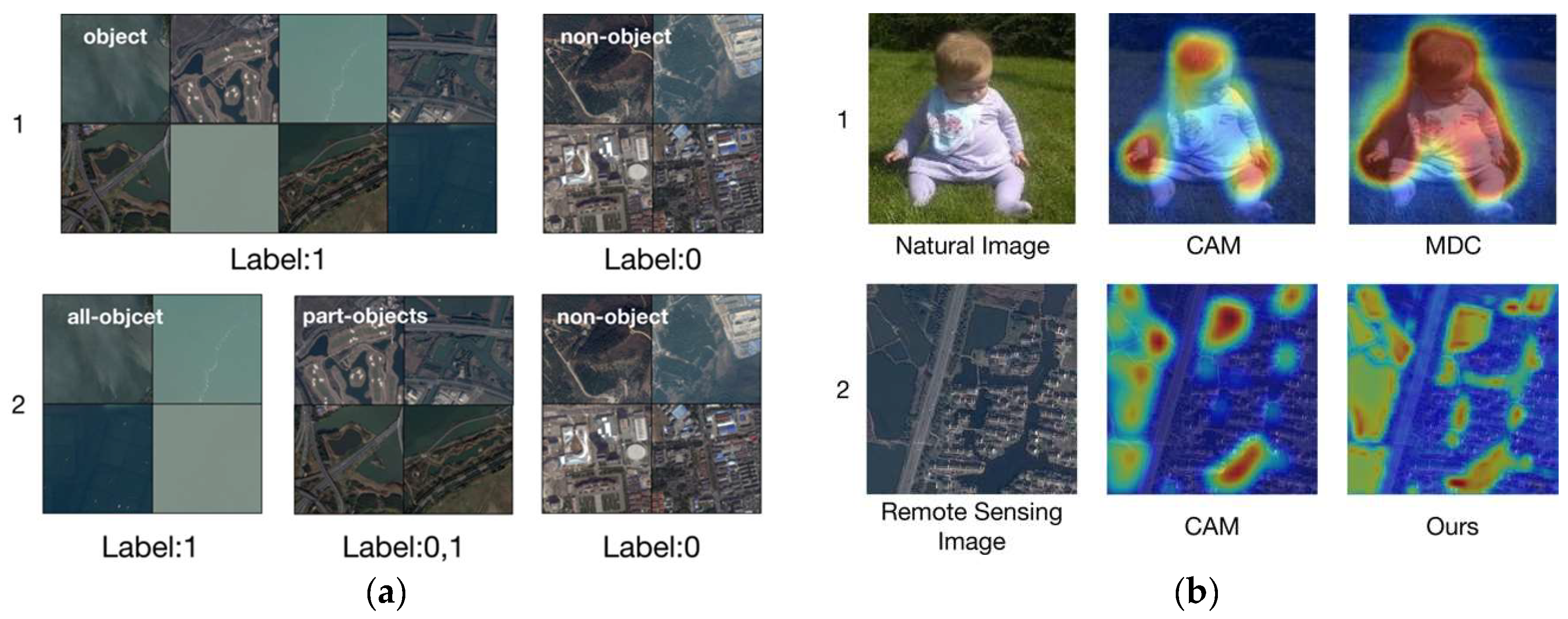
• Unlike computer vision datasets [35,36], remote sensing datasets [6] contain a small number of all-object images. Using the computer vision’s binary classification strategy [22,23] does not make full use of these images, which can lead to the problem of class imbalance. Specifically, as shown in the first row of Figure 1a, the binary classification strategy treats the images as long as they contain objects as one class, and it does not distinguish the all-object images from them. Moreover, too few non-object images are given another label in this case, thus the strategy leads to the problem of class imbalance.
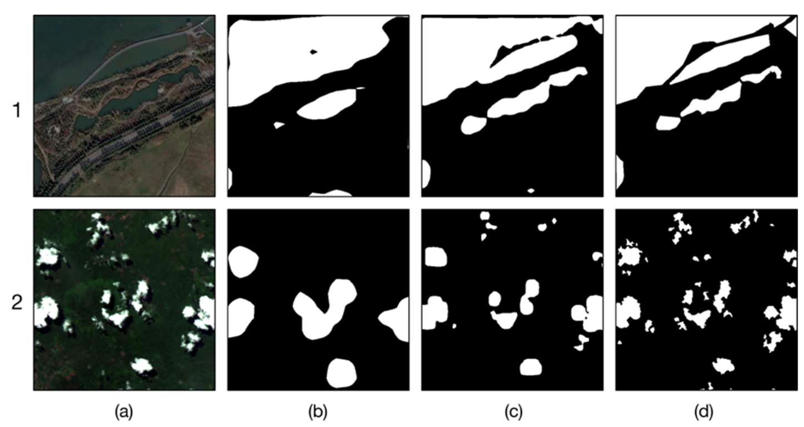
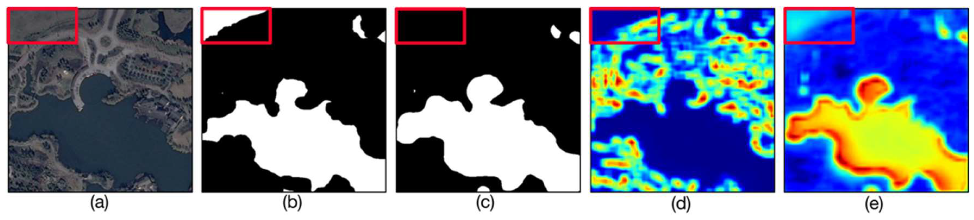
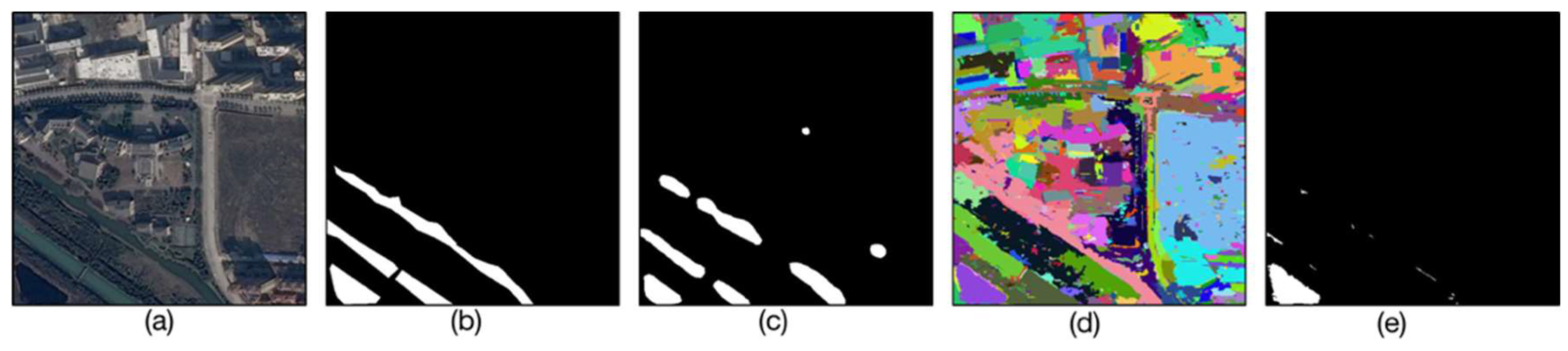
• Object characteristics are different between remote sensing images and natural images. Two kinds of image localization maps produced by the state-of-the-art Class Activation Mapping (CAM) [33] are shown in Figure 1b. Objects in natural images generally consist of multiple parts, thus only some discriminative parts such as head and hands of a child are highlighted by CAM. Therefore, the latest computer vision approaches [20,21] mainly aim at obtaining integral objects, such as Multi-Dilated Convolution (MDC) [20] in Figure 1b. Nevertheless, the main issue in remote sensing images is that the size of objects or background varies greatly in the same image, thus small objects are difficult to identify and a slender background is often sandwiched between two objects by CAM. In addition, remote sensing objects have another characteristic, i.e., some low-level semantics such as water texture and cloud color are obvious, which would be beneficial for localization if they are applied appropriately.

To address the above issue, a novel weakly supervised binary segmentation method is proposed. We first use a Weakly Supervised Feature-fusion Network (WSF-Net) to do classification for generating object regions, which is trained via a balanced binary training strategy. Then, the object regions are provided for training our final segmentation model. Specifically, the main contributions of this work are two-fold:

• A balanced binary classification strategy is proposed to take advantage of all-object images and solve the class imbalance problem caused by binary classification strategy. Our balanced binary classification strategy utilizes this characteristic of remote sensing datasets, as shown in the second row of Figure 1a, thus the class imbalance problem due to the uneven number of object and non-object images can be solved.
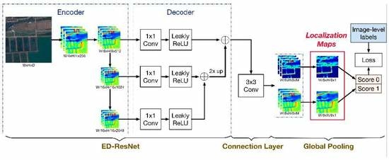
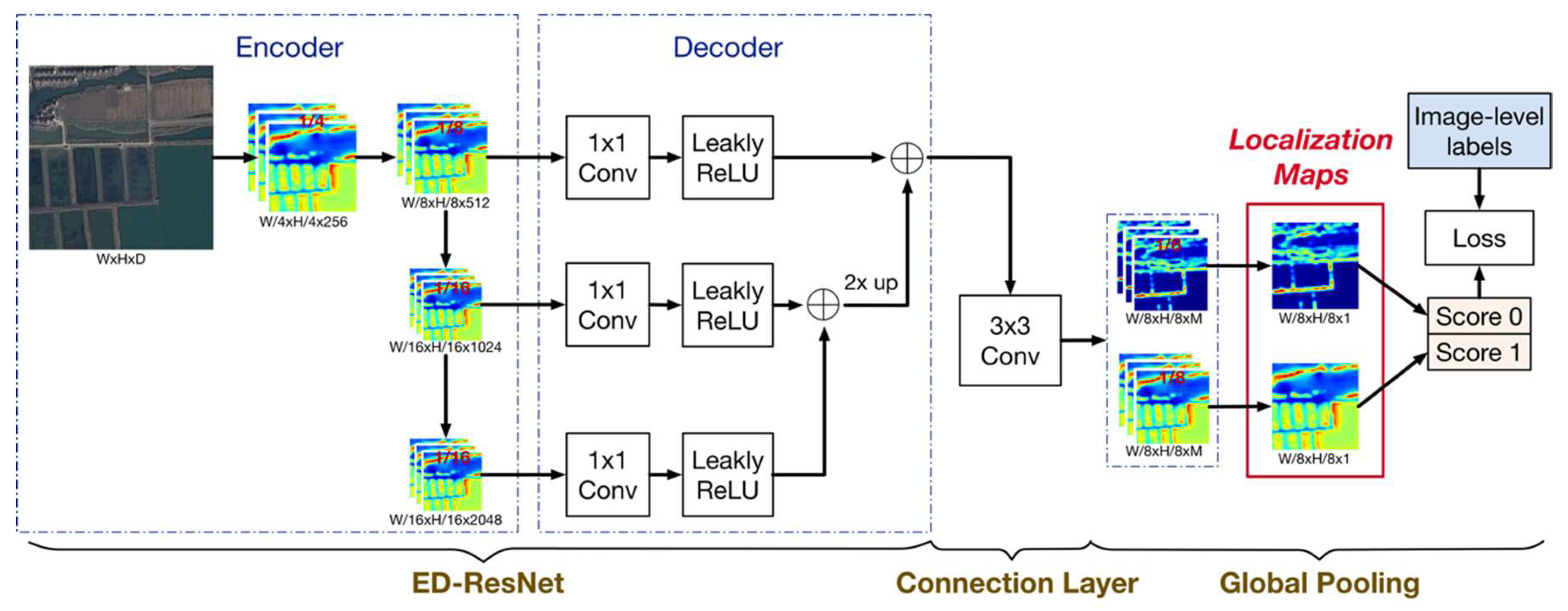
• A WSF-Net that uses a top-down architecture with skip connections is proposed for the unique characteristics of remote sensing objects. In a convolutional network, later layers’ features focus on the category recognition, while early layers’ features can highlight more possible objects due to the high-resolution feature maps and the low-level semantic preference. By combing later layers’ features with early layers’ features, various size objects and background can be observed in the produced localization maps. In Figure 1b, it can be observed that WSF-Net can generate accurate and dense remote sensing object regions for building a good weakly supervised segmentation model.

The rest of this paper is organized as follows. Section 2 describes the architecture of our method in details. Then, the preparation for experiment is presented in Section 3. In Section 4, we present the empirical evaluation of the proposed method on two datasets. The discussion and conclusions are made in Section 5 and Section 6, respectively.

2. Methods

Our weakly supervised binary segmentation method first uses localization approach to obtain object regions, and then object regions are provided to guide segmentation model training. This section first goes into detail about our localization approach, which consists of four parts: (1) a brief review of obtaining object localization through classification; (2) a balanced binary classification strategy for utilizing all-object images; (3) a weakly supervised feature-fusion network for adapting unique remote sensing object characteristics; and (4) a comparison on two selections for generating object regions. After the localization part, we describe how to use the object regions to guide segmentation model training, including a review of the three-phase method, an employment of our object regions in the method, and an improvement for the method.

2.1. Obtain Object Regions via Localization Approach

2.1.1. Brief Review of Localization

Image-level label is common ground truth for training classification network, and it does not provide the classification network with the position of objects in an image. However, Zhou et al. [33] showed that image classification networks can do well in retrieving cues on object localization despite being trained just from image-level labels. Localization ability which classification networks have is proved in Reference [34] through experiments. Convolutional units of classification networks’ layers actually behave as object detectors despite no supervision on the objects’ position, and units of various layers prefer different semantic objects [34]. Early layers, which prefer low-level spatial visual information such as color and texture, can highlight more possible objects, while later layers, which have more category-level evidence and resist the objects’ deformation, have higher accuracy in locating objects.

2.1.2. Balanced Binary Classification Strategy

As described in Section 2.1.1, object regions can be obtained through classification. Most computer vision datasets [35,36] have many object categories such as dog, cat, car, etc., thus they can learn the similarities in the same category and the differences between different categories through multi-class classification to obtain object regions. However, remote sensing datasets generally focus on single a object category (e.g., water and cloud) for most applications, thus the background should be jointed in training classification as another category.

Unlike computer vision datasets [35,36], remote sensing datasets have a particularity: they not only contain images with some objects and images full of background, but also all-object images. We take advantage of this dataset particularity to propose the balanced binary classification strategy. Balanced binary classification strategy sets the label of all-object images as 1 and the label of non-object images as 0, and the images with both object and background have two labels 0 and 1, as shown in the second row of Figure 1a.

Compared with our balanced binary classification strategy, binary classification strategy used in computer vision single-class classification does not make full use of the particularity. It sets the image-level label of an image as 1 as long as the image contains the objects, and an image’s label is considered to be 0 if the image does not contain objects at all as shown in the first row of Figure 1a. Tsutsui et al. [22], using binary classification strategy, added abundant non-object images from extra natural datasets as distant supervisors to complete classification. However, finding such suitable datasets is difficult and inconvenient in remote sensing, thus we only use our datasets for training. Nevertheless, our datasets have a few non-object images, so the binary classification strategy can lead to the problem of class imbalance.

2.1.3. Weakly Supervised Feature-Fusion Network (WSF-Net)

WILDCAT was proposed by Durand et al. in 2017 [32]. It is the state-of-the-art localization network, which is famous for having a logical architecture and being stable on different datasets. The network uses a ResNet [37] to extract features, and then the last layer’s feature dimension is reduced for global pooling to obtain each class’s localization map and score. Although WILDCAT is already powerful in natural image, it cannot give great performance on remote sensing image. Similar to most computer vision approaches [20,21,22,33], WILDCAT only employs ResNet’s last layer’s feature maps to generate localization maps. Such localization maps cannot adapt to the two characteristics of remote sensing images. First, objects and background have various sizes. In the small last feature maps, small objects are difficult to be identified, and two independent objects are easily merged into a single object region. Therefore, higher resolution feature maps are required to address this obstacle. Second, remote sensing objects have some low-level semantics (e.g., water texture and cloud color). Nevertheless, last layer’s features, which pay more attention to high-level semantics (i.e., category-level evidence), lack low-level spatial visual information. Therefore, features which prefer low-level semantics are demanded to locate more possible remote sensing objects’ positions.

According to Zhou et al. [34], early layers’ feature maps, which have higher resolution and prefer low-level semantics, satisfy the two characteristics of remote sensing image, thus combining low-resolution, high-level feature maps with high-resolution, low-level ones can enhance the performance and obtain dense and accurate object localization in remote sensing.

Based on the above observation, we propose a weakly supervised feature-fusion network (WSF-Net) for obtaining localization maps using image-level labels. Figure 2 shows the overall WSF-Net architecture. To enhance the performance, the architecture contains three levels: (1) an Encoder–Decoder ResNet (ED-ResNet) to extract and merge different level features; (2) a connection layer to encode first level’s output and alleviate aliasing effect; and (3) a global pooling to obtain each class localization map and score.

Our ED-ResNet consists of two parts: encoder and decoder. The encoder part is based on ResNet-101, which is applied for extracting features of input data, and the stride of the last stage’s first block is set to 1 to prevent the resolution of the smallest feature maps from being too small. Random scales of remote sensing images are accepted in WSF-Net. We note W $\times$ H $\times$ D as the size of the image. Then, the input layer is followed by a convolutional layer and a max pooling layer, and both of them have stride 2 reducing the size of feature maps to one fourth. After that, four stages are followed and every stage includes several residual blocks. Size of feature maps in the same stages is the same, and feature maps’ size of the following stages is half that of the previous ones in the first three stages. Therefore, the size of the third stage’s feature maps is W/16 $\times$ W/16 $\times$ 512. The stride of the last stage’s first block is set to 1, so that it naturally preserves the resolution of WSF-Net’s smallest feature maps at W/16 $\times$ H/16. As mentioned above, combining low-level feature maps with high-level ones to generate bigger and finer localization maps can obtain dense and accurate object localization, so we add a decoder based on the encoder. In the decoder part, we first simply attach a 1 $\times$ 1 convolutional layer and a leaky ReLU on the second, third, and fourth stages’ outputs, respectively, to reduce the number of channels to keep all decoder layers’ feature dimensions not too high. In this paper, the feature dimension is set to 256, thus all layers in decoder have 256-channel outputs. Then, the third channel-reduced maps are fused with the fourth channel-reduced maps by element-wise addition. After this, the spatial resolution of the fused feature maps is upsampled by a factor of 2 with bilinear upsampling, and then the upsampled maps is fused with the second channel-reduced maps by element-wise addition. Finally, the second, third, and fourth stages’ output feature maps are fused together, and the final feature maps, which have the size of W/8 $\times$ H/8 $\times$ 256, are obtained as the output of ED-ResNet.

After ED-ResNet, a connection layer is needed to connect the previous output and subsequent multiple class-related modalities. Moreover, our ED-ResNet has the aliasing effect caused by the upsampling and element-wise addition operations. For both reasons, a 3 $\times$ 3 convolutional layer are used on ED-ResNet’s output which not only encodes the ResNet’s output into M feature maps per class but also reduces the aliasing effect. Our dataset has two categories, and the feature maps’ size after the connection layer is W/8 $\times$ H/8 $\times$ 2M.

Due to the image-level labels, we use a global pooling as WILDCAT to gather all information contained in the feature maps. First, M maps for two classes are combined independently by average pooling to yield localization maps, and then the maps are transformed from W/8 $\times$ H/8 $\times$ 2M to W/8 $\times$ H/8 $\times$ 2. Second, a spatial pooling module is implemented on each localization map to obtain each class’s score, and then scores are sent to a multi-label logistic loss with the image-level labels.

2.1.4. Generate Object Regions

The localization maps are extracted before spatial pooling. There are two strategies to generate object regions. The first computes the object regions by taking the class with maximum score at each spatial position independently [32]. We call it max-scored category strategy for simplicity. The second, which is called thresholding strategy, selects the pixels belonging to the top $\mathsf{\delta }$% of the largest value in object localization map as their respective object regions [33]. Different thresholds have shown different performance [20,22], especially for various datasets.

2.2. Segmentation Model Training with Object Regions

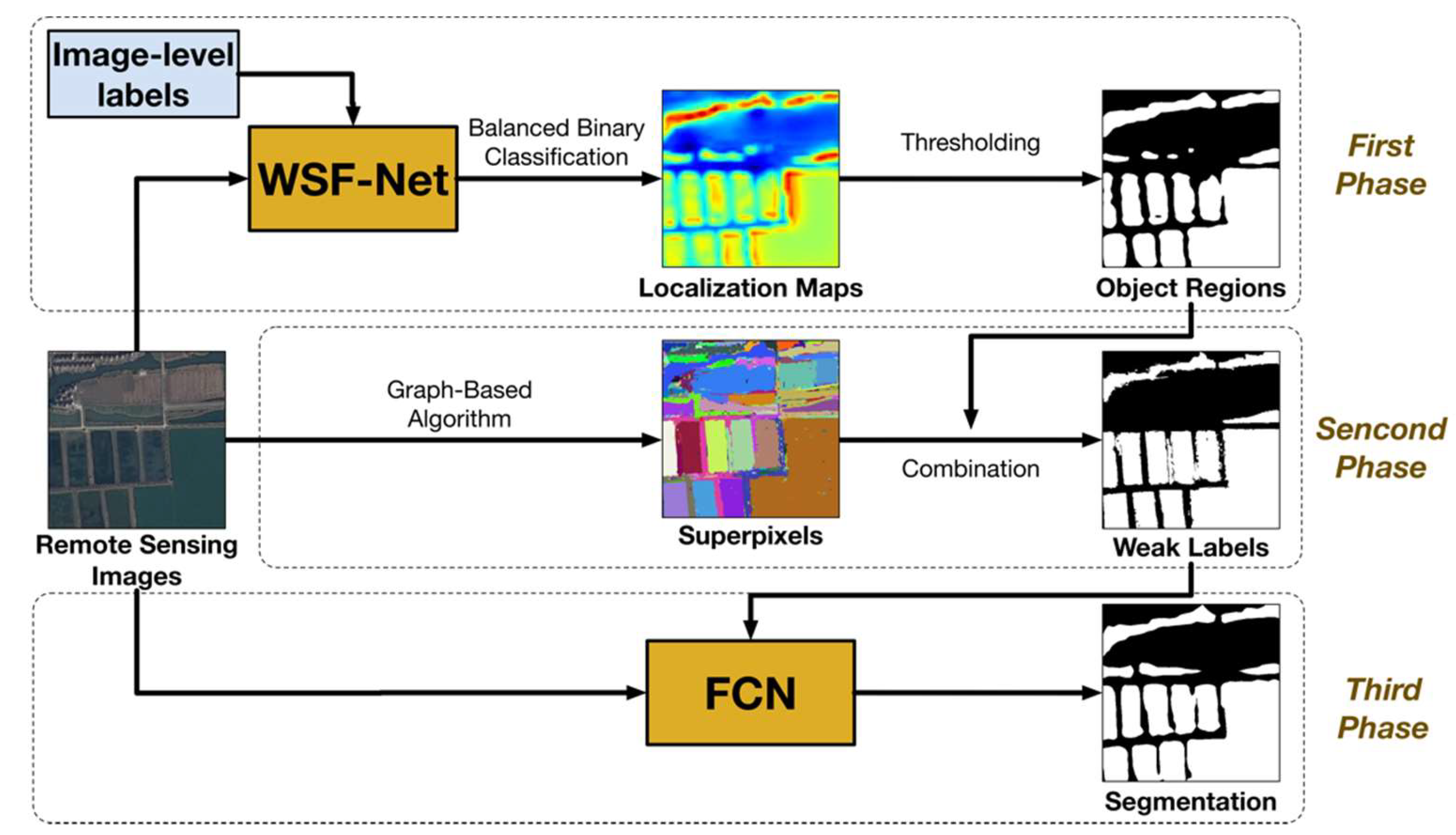
2.2.1. Review of the Three-Phase Method

As introduced in Reference [22], the three-phase method consists of three phases for weakly supervised segmentation model training. An overview of the three-phase method is shown in Figure 3. In the first phase, object regions are obtained for the following phases. Next, object regions are not sufficiently fine-grained as ground truth for training segmentation model to predict the sharp edge of objects, while superpixels mainly rely on low-level features, which are good at portraying the edges of each part. Therefore, superpixels, which are generated by a graph-based algorithm [38], are used to combine with object regions to generate weak labels. For each superpixel, if the overlap with the object regions is greater than a threshold, it is regarded as corresponding to an object. Lastly, weak labels are applied as ground truth for training FCN to obtain a weakly supervised segmentation model. It should be noted that every architecture of FCN can be used in the last phase, and DeepLabV2 [39] architecture without conditional random field (CRF) is utilized as the FCN in our paper. Labels for the three training phases are just image-level annotations. In the testing process, images only need to be sent to the segmentation model to get the segmentation results.

Due to still a gap between weakly supervised and fully supervised quantity, Tsutsui et al. [22] were interested in using a small amount of pixel-level annotations to enhance the segmentation performance. Therefore, the weakly supervised segmentation model is used as pre-trained model, and then pixel-level labels are employed to fine-tune it. A small number of pixel-level labels utilized to train the network can reach the performance of fully supervised model, which also achieves the effect of reducing annotation costs.

2.2.2. Object Regions Obtained by Our Localization Approach Used in the First Phase

A set of object regions is a cornerstone for guiding a weakly supervised segmentation model training. Object regions generated by conventional localization approaches [32,33] are considered reliable only for a small number of large objects’ positions, so they are not enough to obtain comprehensive remote sensing segmentation. With our proposed localization approach, the object regions become denser and more powerful for the following phases’ segmentation model training.

2.2.3. Modify the Strategy of Generating Weak Labels in the Second Phase

Since remote sensing images are more complex than the car centric road images in Reference [22], remote sensing images are oversegmented to obtain many finely divided superpixels to ensure that more objects can be separated from the background. Therefore, using the strategy in Reference [22] results in losing many tiny target superpixels and has a negative impact. We modify it to the following strategy. Let $P$ denote the localization cues and $S$ a set of superpixels; then, the weak label $y_{weak}^{\left(i\right)}$ at location $i$ is defined as:

$$y_{weak}^{\left(i\right)}=\{\begin{array}{c}\mathrm{object} \frac{\left|s_i\cap P\right|}{\left|s_i\right|}>\theta \\ \mathrm{background} \mathrm{otherwise}\end{array}, \forall s_i\in S,$$

(1)

where $\theta$ is the overlap threshold. That is, for each superpixel, if the overlap of object regions and the superpixel relative to the superpixel reaches threshold $\theta$, the superpixel is regarded as corresponding to an object area. In our paper, $\theta$ is set to 0.5.

3. Preparation for Experiment

3.1. Datasets

In our experiments, two different remote sensing datasets were used: Water dataset [6] and Cloud dataset. Most publicly accessible datasets cannot support the entirely new method’s training, so we found only the Water dataset [6] to be applicable. To demonstrate the generalization of our method, we constructed a new Cloud dataset for this paper.

3.1.1. Water Dataset

Water dataset of visible spectrum Google Earth images consists of RGB pan-sharpened images. The dataset has 9409 images each with 512 $\times$ 512 pixels and a resolution of 0.5 m/pixel. We randomly select 80% images as training data and the other as test data. Most images focus on rural areas, and the water annotations include lakes, reservoirs, rivers, ponds, paddy, and ditches, while all other objects such as trees, grass, and buildings are treated as the background.

3.1.2. Cloud Dataset

New Cloud dataset has 8705 images from Gaofen-1 satellite, which are all level-2A products and consist of four bands, including blue, green, red and infrared. Each image contains 512 $\times$ 512 pixels with a resolution of 16 m/pixel. The cloud annotations include thick clouds and thin clouds, while the other objects, such as snow, white buildings, and trees, are treated as the background. Of these dataset images, 80% were used for training and 20% for testing.

For these two datasets, pixel-level labels and image-level labels are provided. Regarding pixel-level labels, the water or cloud pixels are positive, and the background objects pixels are negative. Image-level labels are divided into three kinds, as shown in the second row of Figure 1b: non-object image’s label is set to 0, all-object image’s label is set to 1, and the image with both object and background has two labels, 0 and 1.

3.2. Annotation Cost

Reducing the annotation cost is our work’s fundamental motivation, so we evaluated the annotation time for pixel-level labels and image-level labels. Polygonal lasso tool in Adobe Photoshop CS6 was utilized to delineate objects for generating pixel-level labels. For each pixel-level label, we started timing from the moment that the image was placed in Photoshop and stopped timing until we finished the annotation and saved the label. In this way, the annotation time for each pixel-level label was obtained. Since the datasets we obtained are already annotated, we randomly selected 100 images from each dataset to measure the annotation time. Finally, each dataset’s annotation cost was obtained by averaging the annotation time of 100 images. The average annotation cost for a pixel-level label was estimated to be 129.67 s for a water image (512 $\times$ 512 pixels in size) and 199.78 s for a cloud image (512 $\times$ 512 pixels in size). Therefore, annotation time for 9409 water training images was 9409 $\times$ 129.67 = 1,220,065.03 s $\approx$ 338.91 h and for 8705 cloud training images was 8705 $\times$ 199.78 = 1,739,084.9 s $\approx$ 483.08 h. On the other hand, annotation cost for image-level labels was to determine which kind the image belongs to, thus the annotation time for each water and cloud image was equal based on the estimation. The annotation time was 1 s per image (512 $\times$ 512 pixels in size), thus the total time was 9409 $\times$ 1 = 9409 s $\approx$ 2.61 h for water dataset and 8705 $\times$ 1 = 8705 s $\approx$ 2.42 h for cloud dataset. Therefore, pixel-level labels cost 338.91 h compared to 2.61 h for image-level labels for Water dataset, and the two annotations’ time for Cloud dataset were 483.08 h and 2.42 h, respectively. For fine-tuning with pixel-level labels, the ratio of fully supervised segmentation masks was utilized to calculate the annotation cost for part of pixel-level labels, and then it was added the image-level labels’ cost. For example, 0.4 $\times$ 9409 $\times$ 129.67 + 9409 $\times$ 1 = 497,435.01 s $\approx$ 138.18 h was the annotation cost when 40% of pixel-level labels and all image-level labels of Water dataset were used.

3.3. Implementation

WSF-Net was implemented with PyTorch [40]. The batch size was set to 14, and fixed learning rate was 0.01. DeeplabV2 was employed in the third phase as the FCN was implemented with the publicly available TensorFlow [41] framework. The batch size was set to 6, and basic learning rate was 0.001, which dropped by a factor of 10 every 2000 iterations. Both networks were trained with mini-batched Stochastic Gradient Descent (SGD) with momentum = 0.9 and weight decay = 0.0005. Due to the uniform size of training images, all input into the two networks was size 512 × 512 in the experiments, however, both networks are actually adaptable for any input size in terms of networks structure.

3.4. Evaluation

For both quantitative localization and segmentation performance evaluation, we utilized mean Intersection-Over-Unions (mIOU), Overall Accuracy (OA), Detection Accuracy (DA) and False Alarm Rate (FAR). mIOU and OA are used to measure the overall performance, DA presents the performance of the object, and FAR shows the performance of the background.

IOU, also known as the Jaccard index, is a representation of the ratio of the overlap and the union of the prediction and ground truth, and mIOU, which is widely used in segmentation, is the averaging of the IOU of the object and the background.

$$\mathrm{mIOU}=\frac{1}{2}(\frac{\mathrm{TP}}{\mathrm{TP}+\mathrm{FP}+\mathrm{FN}}+\frac{\mathrm{TN}}{\mathrm{TN}+\mathrm{FP}+\mathrm{FN}}),$$

(2)

OA is the normalization of the trace from the confusion matrix:

$$\mathrm{OA}=\frac{\mathrm{TP}+\mathrm{TN}}{\mathrm{TP}+\mathrm{TN}+\mathrm{FP}+\mathrm{FN}},$$

(3)

DA describes the sensitivity of method to the object:

$$\mathrm{DA}=\frac{\mathrm{TP}}{\mathrm{TP}+\mathrm{FN}},$$

(4)

FAR indicates how the method treats the background as object:

$$\mathrm{FAR}=\frac{\mathrm{FP}}{\mathrm{FP}+\mathrm{TN}}$$

(5)

Here, TP is the number of true positive, TF is the number of true negative, and FP and FN represent false positive and false negative, respectively. These metrics can be calculated by a pixel-based accumulated confusion matrix. For the first three metrics, a score of 0 means complete mismatch, whereas 1 is complete overlap, and a higher score represents a better performance. FAR is the opposite, i.e., a higher score represents a worse performance.

According to Durand et al. [32] and Zhou et al. [33], the localization performance is evaluated with the point-based object localization metric. However, this metric requires bounding box annotations, which are not provided in our datasets, and it is less sensitive to misalignments compared to mIOU. In our study, we pursued obtaining more accurate and complete object regions, so we used a more rigorous metric mIOU, the same as Reference [22], and auxiliary metrics OA, DA, and FAR to evaluate the localization performance.

4. Experimental Results

The experimental setup was a two-part experiment on two remote sensing datasets: Water dataset and Cloud dataset. First, to show our localization approach’s effectiveness, model analysis with each proposed strategy and comparison with other localization approaches are reported. Second, our weakly supervised remote sensing segmentation model trained with object regions was compared with other weakly and fully segmented models.

4.1. Localization Approach

4.1.1. Model Analysis

As mentioned in Section 2.1, three strategies are introduced in our localization approach: (1) it employs balanced binary classification to make full use of all-object images and solve the problem of class imbalance resulted from binary classification; (2) it uses WSF-Net to fit unique remote sensing object’s characteristics and improve WILDCAT’s performance; and (3) it replaces max-scored category strategy to thresholding strategy to select object regions from localization maps. We chose threshold at 20% on Water dataset and 0% on Cloud dataset when the thresholding strategy was used. We evaluated how each of these strategies affects test set performance. Thus, four variations of the proposed approach were considered (

Table 1. Variations of our proposed approach. BC, binary classification; BBC, balanced binary classification; Th, thresholding; WSFN, WSF-Net; MC, max-scored category.

Abbreviation	Description
BC-WILDCAT-Th	Binary classification + WILDCAT + Thresholding
BBC-WILDCAT-Th	Balanced binary classification + WILDCAT + Thresholding
BBC-WSFN-Th (WSL)	Balanced binary classification + WSF-Net + Thresholding
BBC-WSFN-MC	Balanced binary classification + WSF-Net + Max-scored category

), and among them, BBC-WSFN-Th is our final localization approach. For convenience, we use WSL (Weakly Supervised Localization) to indicate it.

Table 2. Results of four variations on the Water dataset test set.

Method	mIOU	OA	DA	FAR
BC-WILDCAT-Th	78.02	90.66	82.13	6.68
BBC-WILDCAT-Th	79.26	91.11	81.27	5.57
BBC-WSFN-Th (WSL)	85.88	94.32	89.96	4.32
BBC-WSFN-MC	79.87	91.60	84.68	6.29

and

Table 3. Results of four variations on the Cloud dataset test set.

Method	mIOU	OA	DA	FAR
BC-WILDCAT-Th	77.49	89.89	85.51	8.65
BBC-WILDCAT-Th	79.99	91.07	86.46	7.32
BBC-WSFN-Th (WSL)	87.14	94.42	90.11	3.93
BBC-WSFN-MC	86.32	94.20	91.73	5.91

presents the results of four variations on the test set of Water and Cloud datasets, respectively.

Balanced Binary Classification: For single-class classification task, there are two strategies to solve this issue, that is, binary classification and balanced binary classification, as mentioned in Section 2.1.2. We experiment two strategies on Water and Cloud datasets to show the benefit of balanced binary classification. In Table 2 and Table 3, BBC-WILDCAT-Th on Water and Cloud datasets yields 76.62 points mIOU and 79.99 points mIOU, and it outperforms BC-WILDCAT-Th by over 1.24 points mIOU and 2.50 points mIOU. The overall accuracy of BBC-WILDCAT-Th in both Water and Cloud datasets also increased by 0.45 points and 1.18 points. We argue that this is because balanced binary classification strategy takes advantage of the particularity of remote sensing datasets, thus the all-object images bring more information for classification. Moreover, remote sensing datasets only have a small number of non-object images, thus binary classification can easily lead to the problem of class imbalance, while our strategy alleviates this problem.

WSF-Net: Our proposed WSF-Net uses a top-down architecture with skip connections, as shown in Figure 2. In Table 2 and Table 3, we can see that WSF-Net instead of WILDCAT significantly improves performance (e.g., BBC-WSFN-Th is better than BBC-WILDCAT-Th by 6.62 points mIOU and 7.15 points mIOU on Water and Cloud datasets, respectively). Both water and cloud qualitative results are visualized in Figure 4, and we can see that object regions of BBC-WILDCAT-Th can be used as rough segmentation results. WILDCAT can only identify the discriminative and big object, and it is easy to misclassify the background between two objects, which is not sufficiently dense and accurate for guiding the following segmentation model. These results may be caused by the small size of localization maps, which generated from the last feature maps caused by multiple stages’ convolutional strides. WSF-Net alleviates these phenomena because we enlarge the localization maps by combining multiple layers’ features. Low-level feature maps have higher resolution to help to observe more possible objects and detect the edge more fine-grained, and they prefer low-level semantics (i.e., cloud color and water texture). Some small objects have low-level semantics and do not have very fierce deformation, thus they can be found on shallow feature maps while deep feature maps only slightly highlight them. Thus, we argue that the finer and bigger localization maps generated by fusing multi-level features keep more spatial resolution and locate dense and accurate regions.

Different Object Region’s Selections: In Table 2 and Table 3, BBC-WSFN-Th yields 6.01 points mIOU and 0.82 points mIOU better performance than BBC-WSFN-MC on Water and Cloud datasets, respectively. FAR shows that BBC-WSFN-MC results have more backgrounds treated as objects than BBC-WSFN-Th results. We provide water qualitative results with two selections in Figure 5. Visualization results obtained by selecting the class with maximum score show a problem that many lawns and trees (such as the areas in the red rectangle in Figure 5) are easily misclassified as water, while this situation rarely occurs on the strategy of taking the pixels belonging to top 20%. After analyzing the localization maps, the water-like background region’s score in water localization map is higher than that in background localization map, so the region is selected as water when we use the strategy of selecting the class with maximum score. Nevertheless, if we take the thresholding strategy to select object regions, this water-like background region will not be considered as water, because it does not exceed the top 20% of the largest value.

4.1.2. Comparison with Other Approaches

In

Table 4. Localization comparison between our approach and other approaches on the Water dataset test set.

Method	mIOU	OA	DA	FAR
CAM [33]	76.62	89.00	71.26	2.63
WILDCAT [32] (baseline)	78.02	90.66	82.13	6.68
WSL	85.88	94.32	89.96	4.32

and

Table 5. Localization comparison between our approach and other approaches on the Cloud dataset test set.

Method	mIOU	OA	DA	FAR
CAM [33]	66.69	81.71	61.72	4.66
WILDCAT [32] (baseline)	77.49	89.89	85.51	8.65
WSL	87.14	94.42	90.11	3.93

, we report the localization performance of our proposed approach (WSL) comparing with the state-of-the-art approaches. Visual performance among all three approaches is also provided in Figure 6. The object region selection of three approaches is the thresholding strategy. Experiments on Water and Cloud datasets demonstrate that our approach ranks first in both mIOU score and overall accuracy, and the visual performance shows that object regions obtained by our approach are very close to the pixel-level labels, so they can be used as rough segmentation results. The mIOU of our approach reaches 85.88 points on Water dataset and 87.14 points on Cloud dataset, and the overall accuracy reaches 94.32 points on Water dataset and 94.42 points on Cloud dataset. We can notice that an important improvement between our approach and the two other computer vision approaches, which confirms the effectiveness of our approach for locating remote sensing objects. Comparing CAM and WILDCAT, WILDCAT is more stable than CAM on different datasets. Although CAM has similar performance to WILDCAT on the Water dataset, its mIOU score is 10.80 points worse on Cloud dataset. Therefore, we choose WILDCAT as our baseline, and some strategies are proposed based on WILDCAT to make our localization approach. The results confirm that they greatly improve the performance of obtaining accurate and dense object regions.

4.2. Segmentation Model

4.2.1. Comparison with Models Obtained by Other Methods Using Image-Level Labels

As mentioned in Section 3.2, by changing the three-phase method’s localization approach to WSL in the first phase and modifying its strategy of generating weak labels in the second phase, our weakly supervised binary segmentation method is conducted and the segmentation model can be obtained in the third phase. For convenience, we use WSSM (Weakly Supervised Segmentation Method) to indicate our method. DeepLabV2 [39] architecture without CRF is utilized as the third phase’s FCN in WSSM and the original three-phase method [22].

Table 6. Segmentation comparisons between our model and models obtained by other methods on the Water dataset test set.

Method	mIOU	OA	DA	FAR
SEC [21]	83.37	93.16	88.31	5.32
Three-phase method [22] (baseline)	86.41	94.68	93.84	5.08
WSSM	88.46	95.46	93.01	3.78

and

Table 7. Segmentation comparisons between our model and models obtained by other methods on the Cloud dataset test set.

Method	mIOU	OA	DA	FAR
SEC [21]	77.76	90.23	88.73	8.29
Three-phase method [22] (baseline)	68.04	82.34	61.71	1.90
WSSM	90.28	95.89	93.77	3.32

show the weakly supervised segmentation performance of our segmentation model, and compares our models with other models obtained by SEC [21] and the original three-phase method [22] in Water and Cloud datasets. Figure 7 provides the visual segmentation results obtained from these models.

It can be observed that our segmentation model achieves an mIOU of 88.46 points on Water dataset and 90.28 points mIOU on Cloud dataset, and our model outperforms the other models with image-level labels. Note that the two other models do poorly in Cloud dataset, and this result is likely to be related to the poor performance of their localization approach (CAM), as shown in Table 5. This finding illustrates the importance of our generic localization approach on generating high-quality object regions.

4.2.2. Comparison with Models Obtained by Other Methods Using Pixel-Level Labels

Table 8. Segmentation comparisons between our model and models obtained by other methods on the Water dataset test set.

Method	mIOU	OA	DA	FAR	Annotation Cost (h)
image-level labels
WSSM	88.46	95.46	93.01	3.78	2.61
+ part of pixel-level labels
WSSM-P (40% pixel-level labels)	91.22	96.59	94.25	2.55	138.18
all pixel-level labels
DeeplabV2 [39] (baseline)	91.22	96.58	94.19	2.54	338.91
DC model [7]	-	93.5	-	-	338.91
DeconvNet-RRF [6]	-	96.9	-	-	338.91

and

Table 9. Segmentation comparisons between our model and models obtained by other methods on the Cloud dataset test set.

Method	mIOU	OA	DA	FAR	Annotation Cost (h)
image-level label
WSSM	90.28	95.89	93.77	3.32	2.42
+ part of pixel-level labels
WSSM-P (40% pixel-level labels)	95.42	98.11	96.99	1.38	193.23
all pixel-level labels
DeeplabV2 [39] (baseline)	95.31	98.06	96.74	1.43	483.08

report the results to compare our segmentation models with other fully supervised models. Our models include a weakly supervised one that uses only image-level labels and a model that adds part of pixel-level labels. We call the method that produces the second model WSSM-P. Because DeepLabV2 [39] is utilized as the third phase’s FCN in our methods, DeeplabV2 trained with all pixel-level labels is the fully supervised baseline. Figure 7 also provides the visual segmentation results of fully supervised baseline. Since there are two additional fully supervised models (DC model [7] and DeconvNet-RRF [6]) utilizing Water dataset, we also compare with them.

Experiments on Water and Cloud datasets show the effectiveness of our method with a small amount of annotation cost. Segmentation result, which trained with image-level labels, achieves 96.97% of the fully pixel-level labels’ baseline performance on Water dataset, and it matches 94.60% of the baseline performance on Cloud dataset, while using less than 1% of the annotation cost. Nevertheless, only using the image-level labels is difficult to reach the fully supervised performance entirely, thus we add part of pixel-level labels to improve the score, as mentioned in Section 2.2.1. When only 40% of the pixel-level labels are used for fine-tuning, mIOU score on both datasets is already comparable to the results of the full supervised model, with using only 40% of the annotation cost. This suggests that, when we only have a few pixel-level labels, using weak labels for low cost pre-training can reach a fully supervised model’s performance.

In Table 8, we also report models obtained by two methods that are designed specifically for water segmentation. Especially DeconvNet-RRF [6] is designed for this Water dataset. Comparing with the DC model [7], which uses pixel-level labels, even our weakly supervised segmentation model that only uses image-level annotations improves OA by 1.96 points. Our method has a slight gap with DeconvNet-RRF, because the DeeplabV2 we selected as the third phase’s FCN is inherently inferior to DeconvNet-RRF. Nevertheless, our method hopes to be generic for most datasets, so we do not select a network designed for specific dataset as a baseline. Otherwise, we can also reach DeconvNet-RRF’s performance with part of pixel-level labels.

In the Experimental Section, we first demonstrate our proposed localization approach’s performance in two ways. Model analysis illustrates that each proposed strategy can really improve the localization performance, and comparisons with other approaches present that our approach ranks first among the state-of-the-art localization approaches. After this, our segmentation models are compared with other weakly and fully supervised segmentation models. By comparing with other weakly supervised models, our weakly supervised segmentation model achieves the best performance. Comparisons with other fully supervised segmentation models shows the effectiveness of our methods with a small amount of annotation cost.

5. Discussion

The experimental results have shown that our method can achieve comparable results to fully supervised method. Meanwhile, compared with the state-of-the art weakly supervised segmentation method, our mIOU (88.46) is greater than three-phase method’s mIOU (86.41) by 2.05 points on the Water dataset. On the Cloud dataset, our mIOU (90.28) is greater than three-phase method’s mIOU (68.04) by 22.24 points. We argue that the performance may result from the denser and more accurate object regions, which guide the segmentation model’s training. Table 2 and Table 3 demonstrate the improvements of each strategy in our localization approach: (1) the proposed balanced binary classification makes full use of the datasets particularity and solves the problem of class imbalance; (2) the proposed WSF-Net adapts unique remote sensing objects’ characteristics and expands the resolution of localization maps to increase the quantity of accurate object regions; and (3) thresholding strategy is used to alleviate object-like background region being considered as object.

However, we can see in Table 4 and Table 6 that our localization approach is 9.26 points mIOU higher than CAM on Water dataset, but our segmentation model only outperforms the model from original three-phase method by 2.05 points mIOU. The main reason may come from the inaccurate weak labels. Figure 8 shows the results of each phase of our method;one can notice that our object regions can indicate most objects, while weak labels generated by combining object regions and superpixels sometimes have fewer objects than object regions. As mentioned in Section 2.2.3, although the image has been oversegmented to get many tiny superpixels, some slender or small objects still ca not be separated from the surrounding background, thus these objects and their surrounding background make up big superpixels. For this reason, some objects have been accurately located in object regions, but their big superpixels do not satisfy the combination strategy (as seen in Equation (1)) to be kept in weak labels. Using the incomplete weak labels to train the segmentation model typically affects the improvement of the final segmentation results. In the future, our work will focus on how to generate more accurate weak labels.

6. Conclusions

In this study, we observed the characteristics of remote sensing images and proposed our weakly supervised binary segmentation method including localization approach to produce object regions and segmentation model trained with object regions. The localization approach consists of balanced binary classification strategy to take advantage of the datasets particularity and solve the problem of class imbalance. Besides, to adapt unique characteristics of remote sensing objects, WSF-Net, which uses a top-down architecture with skip connections, is presented. Extensive experiments on Water dataset and Cloud dataset were conducted to analyze our method and compare with the existing techniques. The results demonstrate that our method reaches the performance of fully supervised methods. In the future, the experiments with other classes of remote sensing objects will be added to show that our method can be applied to a wider variety of datasets.

References

1. Wang, H.; Wang, Y.; Zhang, Q.; Xiang, S.; Pan, C. Gated convolutional neural network for semantic segmentation in high-resolution images. Remote Sens. 2017, 9, 466. [Google Scholar] [CrossRef]
2. Xu, Y.; Wu, L.; Xie, Z.; Chen, Z. Building Extraction in Very High Resolution Remote Sensing Imagery Using Deep Learning and Guided Filters. Remote Sens. 2018, 10, 144. [Google Scholar] [CrossRef]
3. Chen, K.; Fu, K.; Yan, M.; Gao, X.; Sun, X.; Wei, X. Semantic Segmentation of Aerial Images with Shuffling Convolutional Neural Networks. IEEE Geosci. Remote Sens. Lett. 2018, 15, 173–177. [Google Scholar] [CrossRef]
4. Wei, X.; Fu, K.; Gao, X.; Yan, M.; Sun, X.; Chen, K.; Sun, H. Semantic pixel labelling in remote sensing images using a deep convolutional encoder-decoder model. Remote Sens. Lett. 2018, 9, 199–208. [Google Scholar] [CrossRef]
5. Zhan, Y.; Fu, K.; Yan, M.; Sun, X.; Wang, H.; Qiu, X. Change Detection Based on Deep Siamese Convolutional Network for Optical Aerial Images. IEEE Geosci. Remote Sens. Lett. 2017, 14, 1845–1849. [Google Scholar] [CrossRef]
6. Miao, Z.; Fu, K.; Sun, H. Automatic Water-Body Segmentation from High-Resolution Satellite Images via Deep Networks. IEEE Geosci. Remote Sens. Lett. 2018, 15, 602–606. [Google Scholar] [CrossRef]
7. Zhuang, Y.; Wang, P.; Yang, Y.; Shi, H.; Chen, H.; Bi, F. Harbor Water Area Extraction from Pan-Sharpened Remotely Sensed Images Based on the Definition Circle Model. IEEE Geosci. Remote Sens. Lett. 2017, 14, 1690–1694. [Google Scholar] [CrossRef]
8. Lin, H.; Shi, Z.; Zou, Z. Maritime Semantic Labeling of Optical Remote Sensing Images with Multi-Scale Fully Convolutional Network. Remote Sens. 2017, 9, 480. [Google Scholar] [CrossRef]
9. Silveira, M.; Heleno, S. Separation between Water and Land in SAR Images Using Region-Based Level Sets. IEEE Geosci. Remote Sens. Lett. 2009, 6, 471–475. [Google Scholar] [CrossRef]
10. Song, Y.; Wu, Y.; Dai, Y. A new active contour remote sensing river image segmentation algorithm inspired from the cross entropy. Dig. Signal Process. 2016, 48, 322–332. [Google Scholar] [CrossRef]
11. Ciecholewski, M. River channel segmentation in polarimetric SAR images. Expert Syst. Appl. Int. J. 2017, 82, 196–215. [Google Scholar] [CrossRef]
12. Yin, J.; Yang, J. A Modified Level Set Approach for Segmentation of Multiband Polarimetric SAR Images. IEEE Trans. Geosci. Remote Sens. 2014, 52, 7222–7232. [Google Scholar]
13. Glasbey, C.A. An Analysis of Histogram-Based Thresholding Algorithms; Academic Press, Inc.: Cambridge, MA, USA, 1993. [Google Scholar]
14. Chen, J.S.; Huertas, A.; Medioni, G. Fast Convolution with Laplacian-of-Gaussian Masks. IEEE Trans. Pattern Anal. Mach. Intell. 1987, 9, 584–590. [Google Scholar] [CrossRef] [PubMed]
15. Kanopoulos, N.; Vasanthavada, N.; Baker, R.L. Design of an image edge detection filter using the Sobel operator. IEEE J. Solid-State Circuits 2002, 23, 358–367. [Google Scholar] [CrossRef]
16. Ok, A.O. Automated detection of buildings from single VHR multispectral images using shadow information and graph cuts. ISPRS J. Photogramm. Remote Sens. 2013, 86, 21–40. [Google Scholar] [CrossRef]
17. Li, E.; Femiani, J.; Xu, S.; Zhang, X.; Wonka, P. Robust Rooftop Extraction from Visible Band Images Using Higher Order CRF. IEEE Trans. Geosci. Remote Sens. 2015, 53, 4483–4495. [Google Scholar] [CrossRef]
18. Li, Z.; Shen, H.; Li, H.; Xia, G.; Gamba, P.; Zhang, L. Multi-feature combined cloud and cloud shadow detection in GaoFen-1 wide field of view imagery. Remote Sens. Environ. 2017, 191, 342–358. [Google Scholar] [CrossRef] [Green Version]
19. Luo, W.; Li, H.; Liu, G.; Zeng, L. Semantic Annotation of Satellite Images Using Author–Genre–Topic Model. IEEE Trans. Geosci. Remote Sens. 2013, 52, 1356–1368. [Google Scholar] [CrossRef]
20. Wei, Y.; Xiao, H.; Shi, H.; Jie, Z.; Feng, J.; Huang, T.S. Revisiting Dilated Convolution: A Simple Approach for Weakly- and Semi- Supervised Semantic Segmentation. Comput. Vis. Pattern Recognit. 2018, arXiv:1805.04574. [Google Scholar]
21. Kolesnikov, A.; Lampert, C.H. Seed, Expand and Constrain: Three Principles for Weakly-Supervised Image Segmentation. In Proceedings of the European Conference on Computer Vision, Amsterdam, The Netherlands, 8–16 October 2016; Springer International Publishing: Cham, Switzerland, 2016; pp. 695–711. [Google Scholar]
22. Tsutsui, S.; Saito, S.; Kerola, T. Distantly Supervised Road Segmentation. In Proceedings of the IEEE International Conference on Computer Vision Workshop, Istanbul, Turkey, 30–31 January 2018; IEEE: Piscataway, NJ, USA, 2018; pp. 174–181. [Google Scholar]
23. Feng, X.; Yang, J.; Laine, A.F.; Angelini, E.D. Discriminative Localization in CNNs for Weakly-Supervised Segmentation of Pulmonary Nodules. In Proceedings of the International Conference on Medical Image Computing and Computer-Assisted Intervention, Quebec City, QC, Canada, 11–13 September 2017; Springer: Cham, Switzerland, 2017; pp. 568–576. [Google Scholar]
24. Pinheiro, P.O.; Collobert, R. From image-level to pixellevel labeling with convolutional networks. arXiv, 2015; arXiv:1411.6228. [Google Scholar]
25. Pathak, D.; Kr¨ahenb¨uhl, P.; Darrell, T. Constrained Convolutional Neural Networks for Weakly Supervised Segmentation. arXiv, 2015; arXiv:1506.03648. [Google Scholar]
26. Bearman, A.; Russakovsky, O.; Ferrari, V.; Li, F.-F. What’s the point: Semantic segmentation with point supervision. In Proceedings of the European Conference on Computer Vision, Amsterdam, The Netherlands, 8–16 October 2016; Springer: Cham, Switzerland, 2016; pp. 549–565. [Google Scholar]
27. Lin, D.; Dai, J.; Jia, J.; He, K.; Sun, J. ScribbleSup: Scribble-Supervised Convolutional Networks for Semantic Segmentation. In Proceedings of the 2016 IEEE Conference on Computer Vision and Pattern Recognition (CVPR), Las Vegas Valley, NV, USA, 26 June–1 July 2016; IEEE Computer Society: Washington, DC, USA, 2016. [Google Scholar]
28. Tang, M.; Djelouah, A.; Perazzi, F.; Boykov, Y.; Schroers, C. Normalized Cut Loss for Weakly-supervised CNN Segmentation. arXiv, 2018; arXiv:1804.01346. [Google Scholar]
29. Dai, J.; He, K.; Sun, J. BoxSup: Exploiting Bounding Boxes to Supervise Convolutional Networks for Semantic Segmentation. arXiv, 2015; arXiv:1503.01640. [Google Scholar]
30. Khoreva, A.; Benenson, R.; Hosang, J.; Hein, M.; Schiele, B. Simple Does It: Weakly Supervised Instance and Semantic Segmentation. arXiv, 2016; arXiv:1603.07485. [Google Scholar]
31. Andrews, S.; Tsochantaridis, I.; Hofmann, T. Support vector machines for multiple-instance learning. In Proceedings of the Neural Information Processing Systems (NIPS), Vancouver, BC, Canada, 8–13 December 2003. [Google Scholar]
32. Durand, T.; Mordan, T.; Thome, N.; Cord, M. WILDCAT: Weakly Supervised Learning of Deep ConvNets for Image Classification, Pointwise Localization and Segmentation. In Proceedings of the IEEE Conference on Computer Vision and Pattern Recognition, Honolulu, HI, USA, 21–26 July 2017; IEEE Computer Society: Washington, DC, USA, 2017; pp. 5957–5966. [Google Scholar] [Green Version]
33. Zhou, B.; Khosla, A.; Lapedriza, A.; Oliva, A.; Torralba, A. Learning Deep Features for Discriminative Localization. arXiv, 2015; 2921–2929arXiv:1512.04150. [Google Scholar]
34. Zhou, B.; Khosla, A.; Lapedriza, A.; Oliva, A.; Torralba, A. Object Detectors Emerge in Deep Scene CNNs. Comput. Sci. 2014. Available online: https://arxiv.org/abs/1412.6856 (accessed on 5 December 2018).
35. Everingham, M.; Gool, L.V.; Williams, C.K.I.; Winn, J.; Zisserman, A. The Pascal Visual Object Classes (VOC) Challenge. Int. J. Comput. Vis. 2010, 88, 303–338. [Google Scholar] [CrossRef]
36. Cordts, M.; Omran, M.; Ramos, S.; Rehfeld, T.; Enzweiler, M.; Benenson, R.; Franke, U.; Roth, S.; Schiele, B. The Cityscapes Dataset for Semantic Urban Scene Understanding. In Proceedings of the IEEE Conference on Computer Vision and Pattern Recognition, Las Vegas, NV, USA, 27–30 June 2016; IEEE Computer Society: Washington, DC, USA, 2016; pp. 3213–3223. [Google Scholar] [Green Version]
37. He, K.; Zhang, X.; Ren, S.; Sun, J. Deep Residual Learning for Image Recognition. In Proceedings of the IEEE Conference on Computer Vision and Pattern Recognition, Las Vegas, NV, USA, 27–30 June 2016; IEEE Computer Society: Washington, DC, USA, 2016; pp. 770–778. [Google Scholar] [Green Version]
38. Felzenszwalb, P.F.; Huttenlocher, D.P. Efficient graphbased image segmentation. IJCV 2004, 59, 167–181. [Google Scholar] [CrossRef]
39. Chen, L.C.; Papandreou, G.; Kokkinos, I.; Murphy, K.; Yuille, A.L. DeepLab: Semantic Image Segmentation with Deep Convolutional Nets, Atrous Convolution, and Fully Connected CRFs. IEEE Trans. Pattern Anal. Mach. Intell. 2018, 40, 834–848. [Google Scholar] [CrossRef] [Green Version]
40. Paszke, A.; Gross, S.; Chintala, S.; Chanan, G.; Yang, E.; DeVito, Z.; Lin, Z.; Desmaison, A.; Antiga, L.; Lerer, A. Automatic differentiation in PyTorch. 2017. Available online: https://openreview.net/forum?id=BJJsrmfCZ (accessed on 5 December 2018).
41. Abadi, M.; Agarwal, A.; Barham, P.; Brevdo, E.; Chen, Z.; Citro, C.; Corrado, G.S.; Davis, A.; Dean, J.; Devin, M.; et al. TensorFlow: Large-Scale Machine Learning on Heterogeneous Distributed Systems. arXiv, 2016; arXiv:1603.04467. [Google Scholar]
Figure 1. (a) Comparison between binary classification strategy (first row) and our balanced binary classification strategy (second row) on Water dataset; and (b) comparison between natural images (first row) and remote sensing images (second row) on object’s characteristics displayed in the localization maps.
Remotesensing 10 01970 g001
Figure 2. The architecture of Weakly Supervised Feature-Fusion Network (WSF-Net). Encoder–Decoder ResNet (ED-ResNet) consists of encoder and decoder to extract and merge different level features of whole images respectively. Then ED-ResNet’s outputs are encoded by the connection layer into M feature maps per class. Finally, feature maps are combined separately to yield localization maps that can be globally pooled to obtain a single score for each class, and then scores are sent to a multi-label logistic loss with the image-level labels.
Remotesensing 10 01970 g002
Figure 3. The overview of three-phase method. From remote sensing images and image-level labels, we first obtain object regions through balanced binary classification with WSF-Net. Then, the object regions are combined with superpixels to generate weak labels in the second phase. The weak labels are used for training an FCN to get the final segmentation model in the third phase.
Remotesensing 10 01970 g003
Figure 4. Results of the object regions with and without WSF-Net on Water dataset (first row) and Cloud dataset (second row): (a) the original remote sensing image; (b) the results of BBC-WILDCAT-Th; (c) the results of BBC-WSFN-Th; and (d) the pixel-level label.
Remotesensing 10 01970 g004
Figure 5. Water qualitative results with two object region’s selections: (a) the original remote sensing image; (b) the result of BBC-WSFN-MC; (c) the result of BBC-WSFN-Th; (d) the background localization map; and (e) the water localization map. The red rectangle represents the water-like background
Remotesensing 10 01970 g005
Figure 6. Results of the object regions between our approach and other approaches on Water dataset (first and second rows) and Cloud dataset (third and fourth rows): (a) the original remote sensing images; (b) the results of CAM (c) the results of WILDCAT; (d) the results of WSL; and (e) the pixel-level label. The red rectangles represent the performance on small objects.
Remotesensing 10 01970 g006
Figure 7. Segmentation results between our model and models obtained by other methods on Water dataset (first and second rows) and Cloud dataset (third and fourth rows): (a) the original remote sensing image; (b) the results of SEC; (c) the results of the original three-phase method; (d) the results of WSSM; (e) the results of DeeplabV2; and (f) the pixel-level label.
Remotesensing 10 01970 g007
Figure 8. Results of each phase of our method on Water dataset: (a) the original remote sensing image; (b) the pixel-level label; (c) the object regions; (d) the superpixels; and (e) the weak labels.
Remotesensing 10 01970 g008