Utilizing Collocated Crop Growth Model Simulations to Train Agronomic Satellite Retrieval Algorithms

Abstract

1. Introduction
1.1. Background
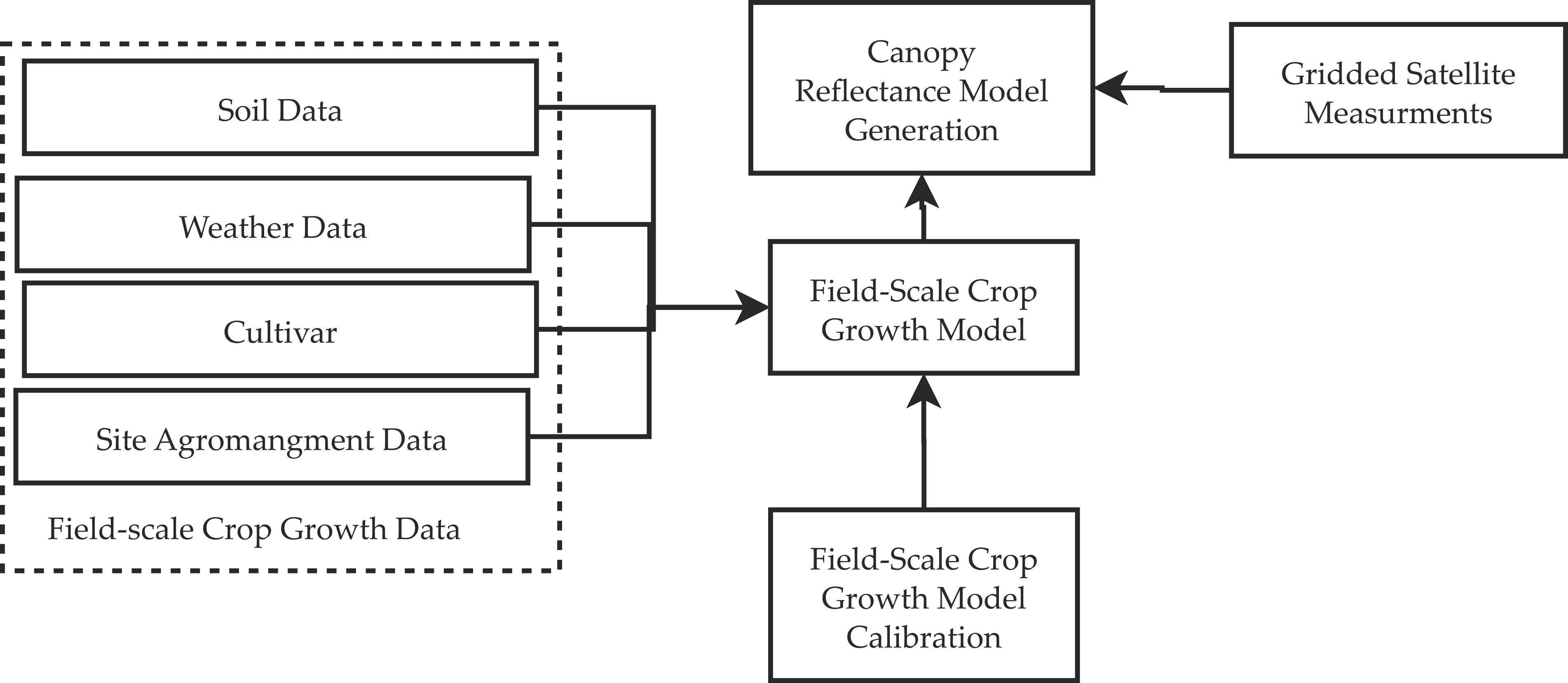
1.2. Overview
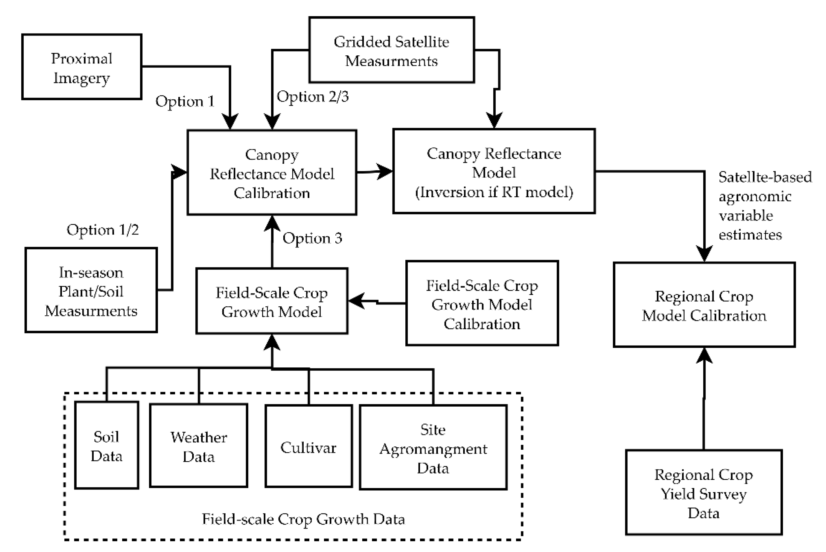
- Optimization of unknown canopy RT model inputs (such as the average leaf angle)
- Optimization of the empirical relationships between crop growth model outputs and canopy RT model inputs
- Optimization of empirical canopy reflectance models that bypass the canopy RT models
- Accurate, geolocated agromanagement data collected by farmers, supplemented by publicly available high-resolution weather and soil datasets, can be used to provide decent estimates of the water and nitrogen-limited attainable state variables at a set of training sites.
- In highly developed cropping systems, such as those in the US Corn Belt, the gap between the attainable yields and the actual yields, which have been further reduced by weeds, pests, and other factors, is sufficiently small that significant information about the attainable state variables is contained in the actual state variables.
- Crop model-predicted state variables at a set of training sites with accurate, geolocated agromanagement data can be used to teach a bidirectional long short-term memory network (BLSTM) to retrieve the attainable state variables solely from the satellite measurements.
2. Materials and Methods
2.1. APSIM-Maize
2.2. Data
2.2.1. Soil Data
2.2.2. Meteorological Data (PRISM and NASA POWER)
2.2.3. Satellite Solar Reflectance Data (MODIS)
2.2.4. USDA NASS Survey Data
2.3. Methods
2.3.1. APSIM Calibration
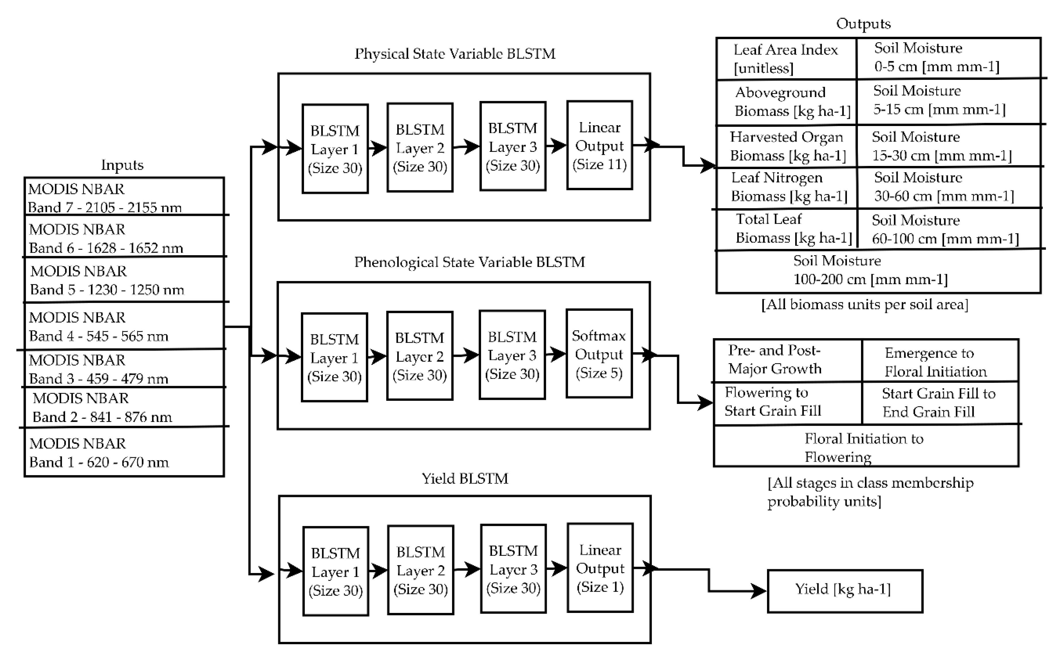
2.3.2. Retrieval of Predicted State Variables from Satellite Measurements
- The physical state variable-predicting BLSTM uses a standard linear output layer and sum of square errors cost function. Each of the physical state variables is normalized to zero mean and unit variance using the training data to ensure that units do not cause the network to favor training one of the state variables over another.
- The yield-predicting BLSTM is trained separately because it is designed to predict a single value for the entire season, rather than a time series. The outputs for all the time steps of the yield-predicting BLSTM are averaged to obtain a single yield value.
- The phenological state variable BLSTM is trained separately because the fraction of fields in each phenological stage in a county is equivalent to the probability that a particular field in a county is in a particular phenological stage. As a result, a softmax output layer, which forces the outputs to be probabilities that sum to 1, and a cross-entropy cost function must be used.
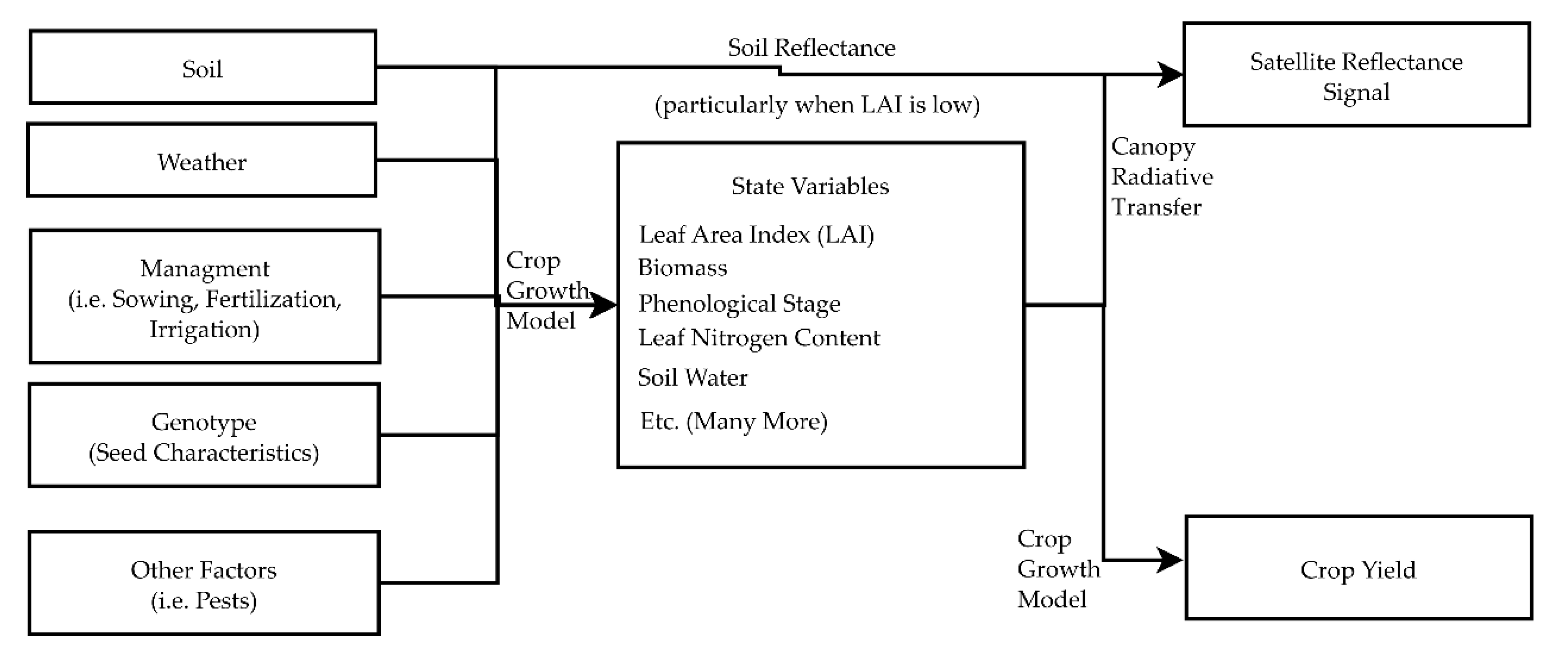
- Variables describing leaf growth and senescence (LAI, total leaf biomass, and leaf nitrogen biomass)
- Variables describing major cumulative carbon assimilation (aboveground biomass and harvested organ biomass)
- Specific leaf area
- Leaf nitrogen percentage
- Soil moisture
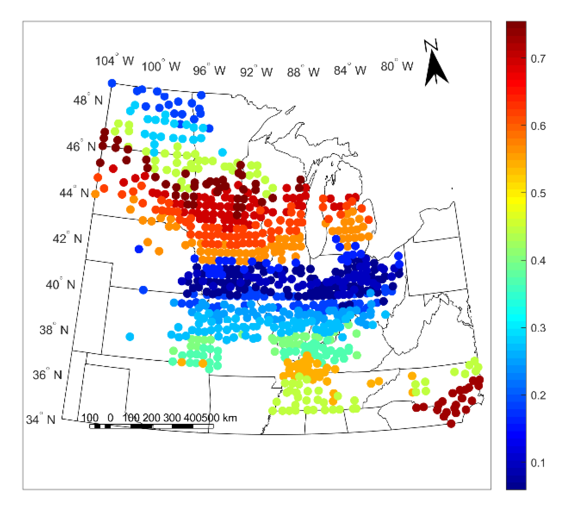
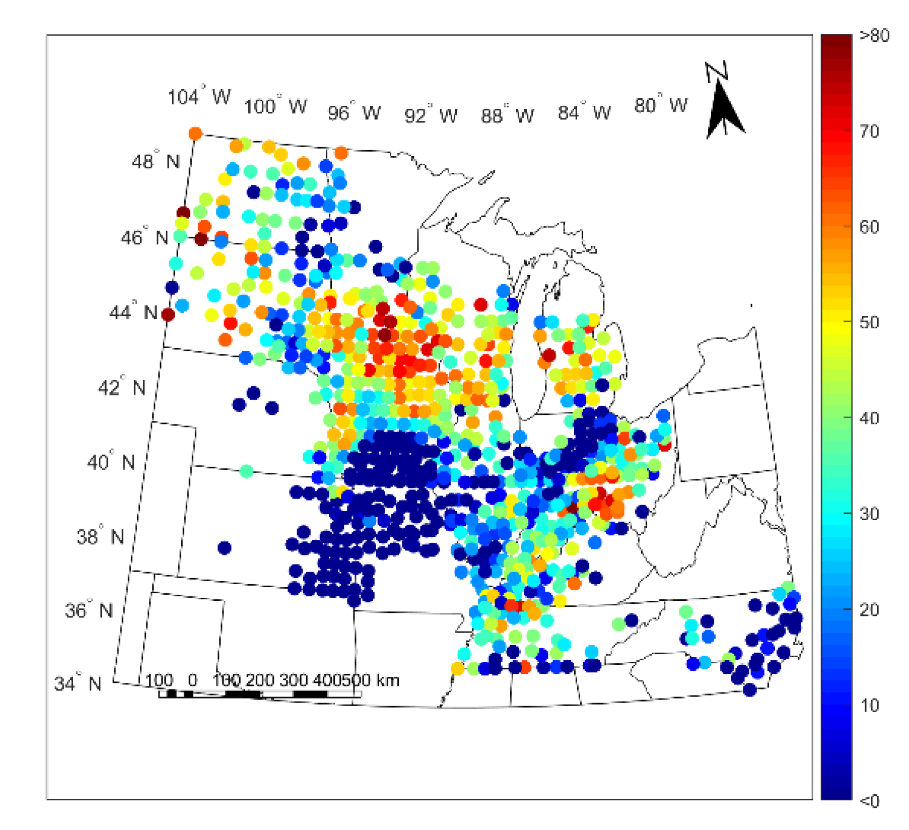
3. APSIM Calibration
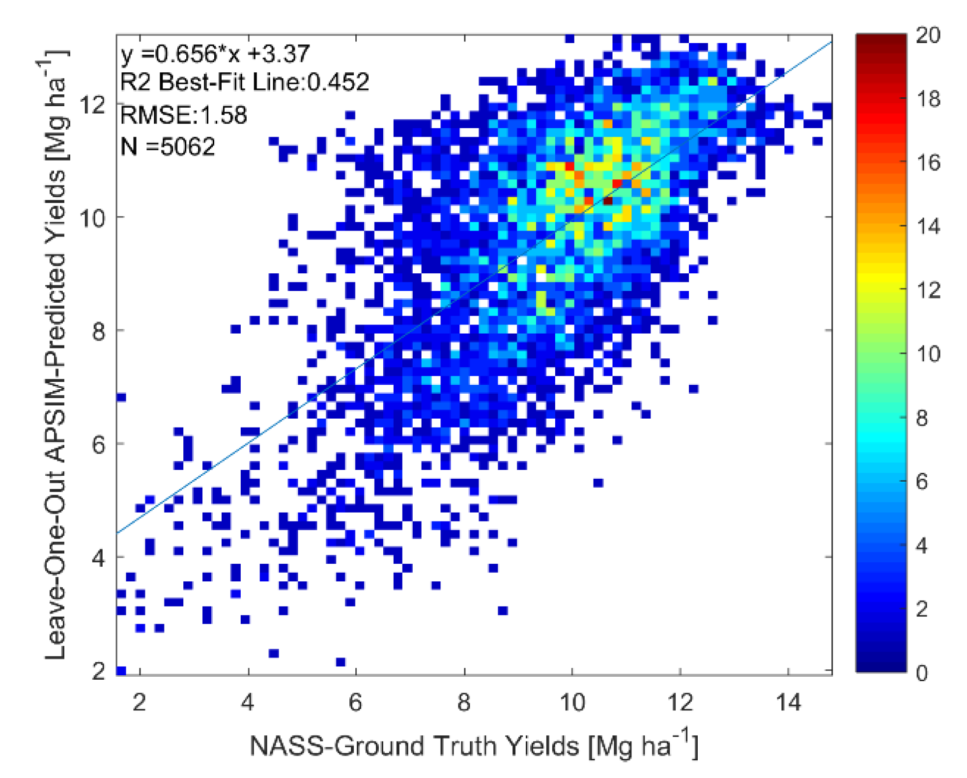
3.1. Results
3.2. Discussion
- It is high when the yield variability is driven by phenomena that are well-modelled and caused by input factors known to the model, such as intracluster variability in weather and soil, as opposed to factors unknown to the model, such as intracluster variability in genotype, agromanagement practices, pests, weeds, and other factors.
- It is high only when the model generalizes to other counties and years in the region, implying a degree of physicality, due to its cross-validated nature
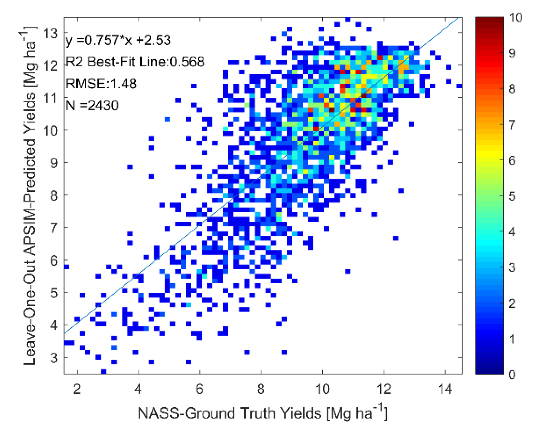
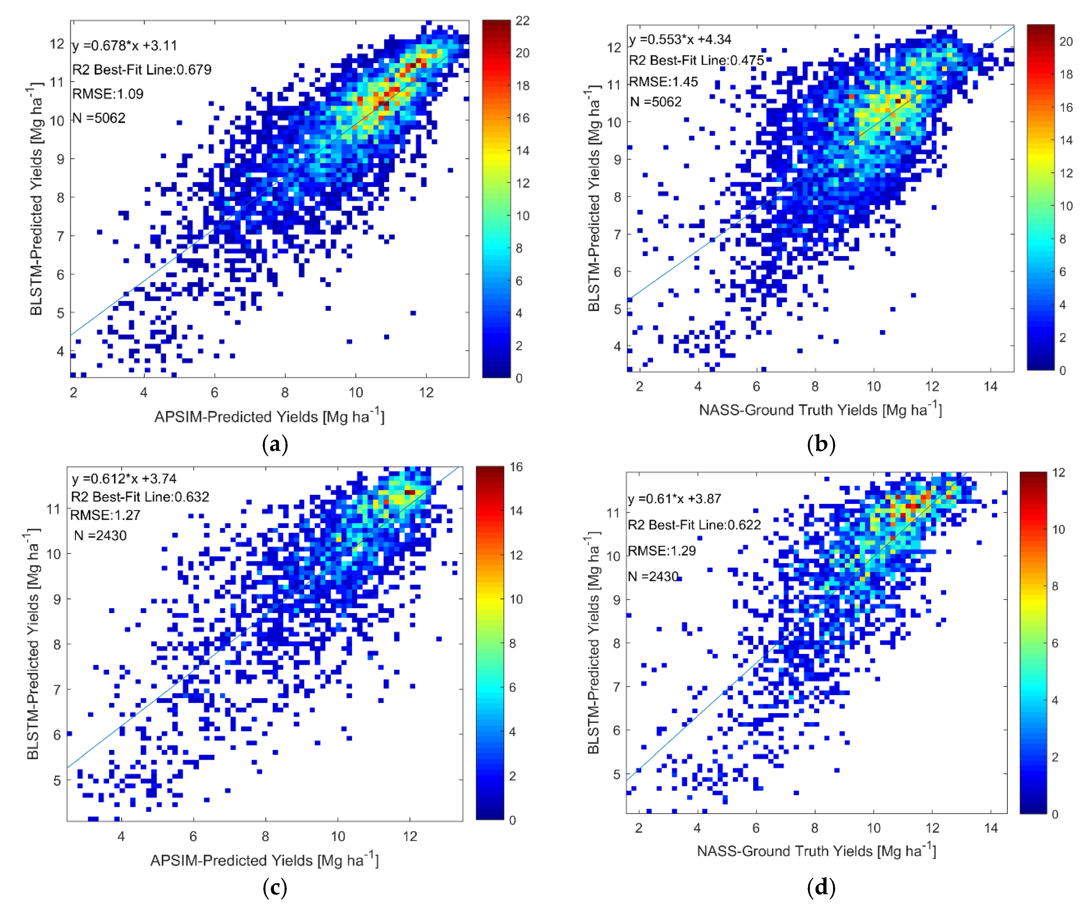
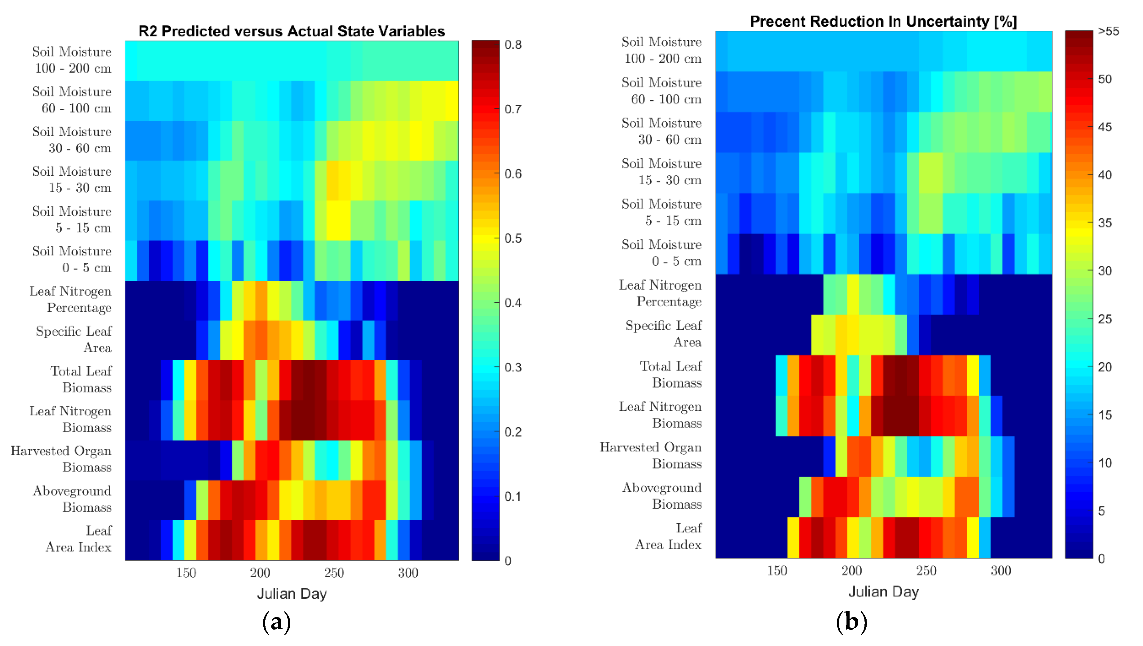
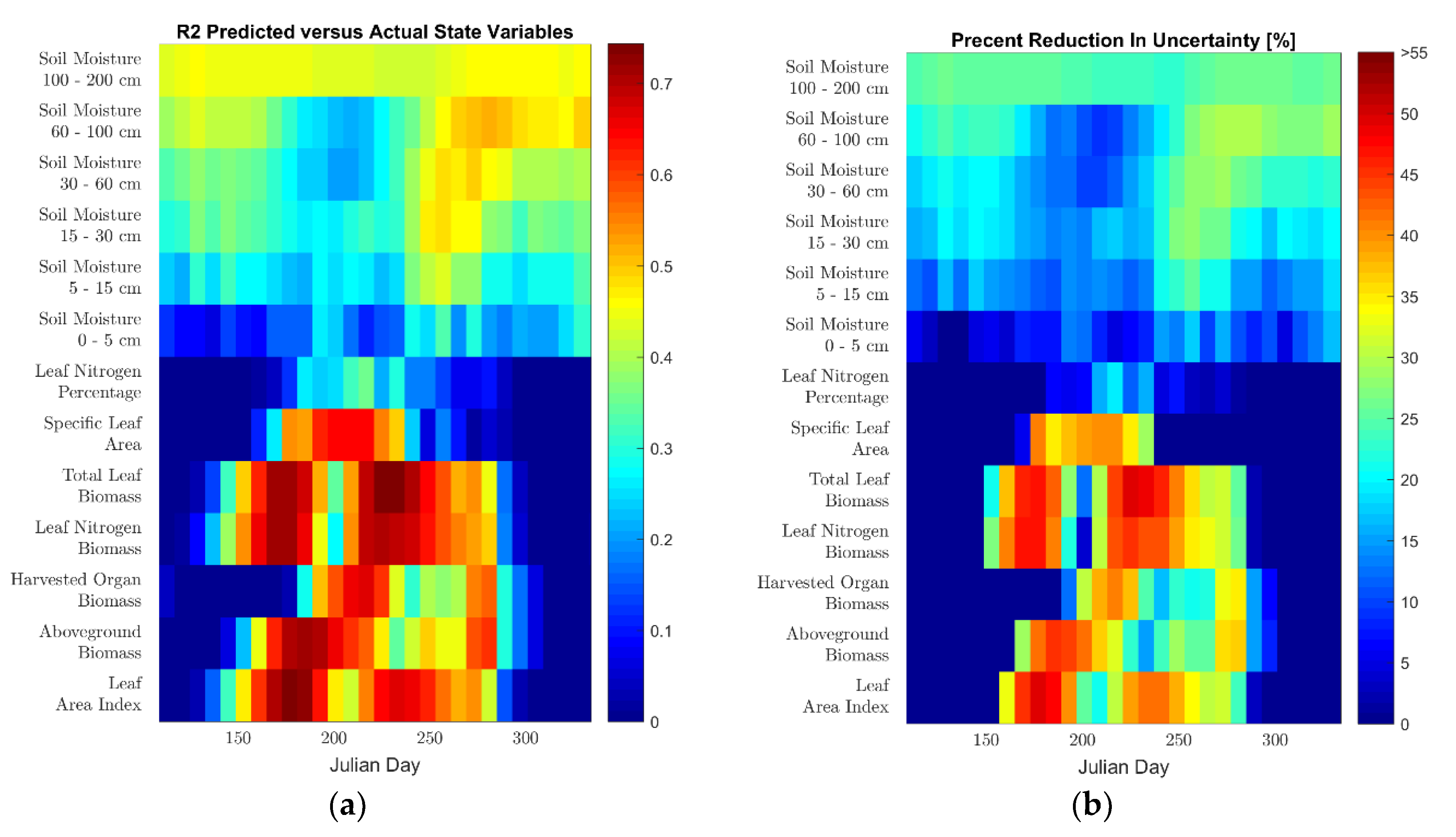
4. Retrieval of Predicted State Variables from Satellite Measurements
4.1. Results
4.2. Discussion
5. Conclusions
Supplementary Materials
Author Contributions
Funding
Acknowledgments
Conflicts of Interest
References
- Levitan, N.; Gross, B. Assessment of the Information Content in Solar Reflective Satellite Measurements with Respect to Crop Growth Model State Variables. In Proceedings of the 14th International Conference on Precision Agriculture, Montreal, QC, Canada, 24–27 June 2018; International Society of Precision Agriculture: Monticello, IL, USA, 2018; pp. 1–12. [Google Scholar]
- Rosenzweig, C.; Elliott, J.; Deryng, D.; Ruane, A.C.; Müller, C.; Arneth, A.; Boote, K.J.; Folberth, C.; Glotter, M.; Khabarov, N.; et al. Assessing agricultural risks of climate change in the 21st century in a global gridded crop model intercomparison. Proc. Natl. Acad. Sci. USA 2014, 111, 3268–3273. [Google Scholar] [CrossRef] [PubMed]
- Lecerf, R.; Ceglar, A.; López-Lozano, R.; Van Der Velde, M.; Baruth, B. Assessing the information in crop model and meteorological indicators to forecast crop yield over Europe. Agric. Syst. 2018, 168, 191–202. [Google Scholar] [CrossRef]
- Woodard, J.D. Integrating high resolution soil data into federal crop insurance policy: Implications for policy and conservation. Environ. Sci. Policy 2016, 66, 93–100. [Google Scholar] [CrossRef]
- Oliver, Y.M.; Robertson, M.J.; Wong, M.T.F. Integrating farmer knowledge, precision agriculture tools, and crop simulation modelling to evaluate management options for poor-performing patches in cropping fields. Eur. J. Agron. 2010, 32, 40–50. [Google Scholar] [CrossRef]
- Grassini, P.; Wolf, J.; Tittonell, P.; Hochman, Z. Yield gap analysis with local to global relevance—A review. Field Crop. Res. 2013, 143, 4–17. [Google Scholar] [CrossRef]
- Huffman, T.; Qian, B.; De Jong, R.; Liu, J.; Wang, H.; McConkey, B.; Brierley, T.; Yang, J.; Jong, D. Upscaling modelled crop yields to regional scale: A case study using DSSAT for spring wheat on the Canadian prairies. Can. J. Soil Sci. 2015, 95, 49–61. [Google Scholar] [CrossRef]
- van Bussel, L.G.J.; Grassini, P.; Van Wart, J.; Wolf, J.; Claessens, L.; Yang, H.; Boogaard, H.; de Groot, H.; Saito, K.; Cassman, K.G.; et al. From field to atlas: Upscaling of location-specific yield gap estimates. Field Crop. Res. 2015, 177, 98–108. [Google Scholar] [CrossRef]
- Deryng, D.; Sacks, W.J.; Barford, C.C.; Ramankutty, N. Simulating the effects of climate and agricultural management practices on global crop yield. Glob. Biogeochem. Cycles 2011, 25. [Google Scholar] [CrossRef]
- Müller, C.; Elliott, J.; Chryssanthacopoulos, J.; Arneth, A.; Balkovic, J.; Ciais, P.; Deryng, D.; Folberth, C.; Glotter, M.; Hoek, S.; et al. Global gridded crop model evaluation: Benchmarking, skills, deficiencies and implications. Geosci. Model Dev. 2017, 10, 1403–1422. [Google Scholar] [CrossRef]
- Morell, F.J.; Yang, H.S.; Cassman, K.G.; Van Wart, J.; Elmore, R.W.; Licht, M.; Coulter, J.A.; Ciampitti, I.A.; Pittelkow, C.M.; Brouder, S.M.; et al. Can crop simulation models be used to predict local to regional maize yields and total production in the U.S. Corn Belt? Field Crop. Res. 2016, 192, 1–12. [Google Scholar] [CrossRef]
- Xiong, W.; Skalský, R.; Porter, C.H.; Balkovič, J.; Jones, J.W.; Yang, D. Calibration-induced uncertainty of the EPIC model to estimate climate change impact on global maize yield. J. Adv. Model. Earth Syst. 2016, 8, 1358–1375. [Google Scholar] [CrossRef]
- Teixeira, E.I.; Zhao, G.; de Ruiter, J.; Brown, H.; Ausseil, A.-G.; Meenken, E.; Ewert, F. The interactions between genotype, management and environment in regional crop modelling. Eur. J. Agron. 2017, 88, 106–115. [Google Scholar] [CrossRef]
- Ewert, F.; van Ittersum, M.K.; Heckelei, T.; Therond, O.; Bezlepkina, I.; Andersen, E. Scale changes and model linking methods for integrated assessment of agri-environmental systems. Agric. Ecosyst. Environ. 2011, 142, 6–17. [Google Scholar] [CrossRef]
- Angulo, C.; Rötter, R.; Lock, R.; Enders, A.; Fronzek, S.; Ewert, F. Implication of crop model calibration strategies for assessing regional impacts of climate change in Europe. Agric. For. Meteorol. 2013, 170, 32–46. [Google Scholar] [CrossRef]
- Tatsumi, K. Effects of automatic multi-objective optimization of crop models on corn yield reproducibility in the U.S.A. Ecol. Model. 2016, 322, 124–137. [Google Scholar] [CrossRef]
- Weiss, M.; Troufleau, D.; Baret, F.; Chauki, H.; Prévot, L.; Olioso, A.; Bruguier, N.; Brisson, N. Coupling canopy functioning and radiative transfer models for remote sensing data assimilation. Agric. For. Meteorol. 2001, 108, 113–128. [Google Scholar] [CrossRef]
- Jacquemoud, S.; Verhoef, W.; Baret, F.; Bacour, C.; Zarco-Tejada, P.J.; Asner, G.P.; François, C. PROSPECT + SAIL models: A review of use for vegetation characterization. Remote Sens. Environ. 2009, 113, S56–S66. [Google Scholar] [CrossRef]
- Houborg, R.; McCabe, M.; Cescatti, A.; Gao, F.; Schull, M.; Gitelson, A. Joint leaf chlorophyll content and leaf area index retrieval from Landsat data using a regularized model inversion system (REGFLEC). Remote Sens. Environ. 2015, 159, 203–221. [Google Scholar] [CrossRef]
- Yu, K.; Lenz-Wiedemann, V.; Chen, X.; Bareth, G. Estimating leaf chlorophyll of barley at different growth stages using spectral indices to reduce soil background and canopy structure effects. ISPRS J. Photogramm. Remote Sens. 2014, 97, 58–77. [Google Scholar] [CrossRef]
- Archontoulis, S.V.; Miguez, F.E.; Moore, K.J. Evaluating APSIM maize, soil water, soil nitrogen, manure, and soil temperature modules in the Midwestern United States. Agron. J. 2014, 106, 1025–1040. [Google Scholar] [CrossRef]
- Kersebaum, K.C.; Boote, K.J.; Jorgenson, J.S.; Nendel, C.; Bindi, M.; Frühauf, C.; Gaiser, T.; Hoogenboom, G.; Kollas, C.; Olesen, J.E.; et al. Analysis and classification of data sets for calibration and validation of agro-ecosystem models. Environ. Model. Softw. 2015, 72, 402–417. [Google Scholar] [CrossRef]
- Hunt, L.A.; Boote, K.J. Data for Model Operation, Calibration, and Evaluation; Springer: Dordrecht, The Netherlands, 1998; pp. 9–39. [Google Scholar]
- Combal, B.; Baret, F.; Weiss, M.; Trubuil, A.; Macé, D.; Pragnère, A.; Myneni, R.; Knyazikhin, Y.; Wang, L. Retrieval of canopy biophysical variables from bidirectional reflectance: Using prior information to solve the ill-posed inverse problem. Remote Sens. Environ. 2003, 84, 1–15. [Google Scholar] [CrossRef]
- Baret, F.; Houles, V.; Guerif, M. Quantification of plant stress using remote sensing observations and crop models: The case of nitrogen management. J. Exp. Bot. 2006, 58, 869–880. [Google Scholar] [CrossRef] [PubMed]
- Duan, S.-B.; Li, Z.-L.; Wu, H.; Tang, B.-H.; Ma, L.; Zhao, E.; Li, C. Inversion of the PROSAIL model to estimate leaf area index of maize, potato, and sunflower fields from unmanned aerial vehicle hyperspectral data. Int. J. Appl. Earth Obs. Geoinf. 2014, 26, 12–20. [Google Scholar] [CrossRef]
- Zhang, L.; Guo, C.L.; Zhao, L.Y.; Zhu, Y.; Cao, W.X.; Tian, Y.C.; Cheng, T.; Wang, X. Estimating wheat yield by integrating the WheatGrow and PROSAIL models. Field Crop. Res. 2016, 192, 55–66. [Google Scholar] [CrossRef]
- Machwitz, M.; Giustarini, L.; Bossung, C.; Frantz, D.; Schlerf, M.; Lilienthal, H.; Wandera, L.; Matgen, P.; Hoffmann, L.; Udelhoven, T. Enhanced biomass prediction by assimilating satellite data into a crop growth model. Environ. Model. Softw. 2014, 62, 437–453. [Google Scholar] [CrossRef]
- Thorp, K.R.; Wang, G.; West, A.L.; Moran, M.S.; Bronson, K.F.; White, J.W.; Mon, J. Estimating crop biophysical properties from remote sensing data by inverting linked radiative transfer and ecophysiological models. Remote Sens. Environ. 2012, 124, 224–233. [Google Scholar] [CrossRef]
- Schlemmer, M.; Gitelson, A.; Schepers, J.; Ferguson, R.; Peng, Y.; Shanahan, J.; Rundquist, D. Remote estimation of nitrogen and chlorophyll contents in maize at leaf and canopy levels. Int. J. Appl. Earth Obs. Geoinf. 2013, 25, 47–54. [Google Scholar] [CrossRef]
- Corti, M.; Cavalli, D.; Cabassi, G.; Marino Gallina, P.; Bechini, L. Does remote and proximal optical sensing successfully estimate maize variables? A review. Eur. J. Agron. 2018, 99, 37–50. [Google Scholar] [CrossRef]
- Sibley, A.M.; Grassini, P.; Thomas, N.E.; Cassman, K.G.; Lobell, D.B. Testing Remote Sensing Approaches for Assessing Yield Variability among Maize Fields. Agron. J. 2014, 106, 24. [Google Scholar] [CrossRef]
- Lobell, D.B.; Thau, D.; Seifert, C.; Engle, E.; Little, B. A scalable satellite-based crop yield mapper. Remote Sens. Environ. 2015, 164, 324–333. [Google Scholar] [CrossRef]
- Jin, Z.; Azzari, G.; Lobell, D.B. Improving the accuracy of satellite-based high-resolution yield estimation: A test of multiple scalable approaches. Agric. For. Meteorol. 2017, 247, 207–220. [Google Scholar] [CrossRef]
- Clevers, J.G.P. A simplified approach for yield prediction of sugar beet based on optical remote sensing data. Remote Sens. Environ. 1997, 61, 221–228. [Google Scholar] [CrossRef]
- Sakamoto, T.; Gitelson, A.A.; Arkebauer, T.J. MODIS-based corn grain yield estimation model incorporating crop phenology information. Remote Sens. Environ. 2013, 131, 215–231. [Google Scholar] [CrossRef]
- Johnson, D.M. A comprehensive assessment of the correlations between field crop yields and commonly used MODIS products. Int. J. Appl. Earth Obs. Geoinf. 2016, 52, 65–81. [Google Scholar] [CrossRef]
- Soufizadeh, S.; Munaro, E.; McLean, G.; Massignam, A.; van Oosterom, E.J.; Chapman, S.C.; Messina, C.; Cooper, M.; Hammer, G.L. Modelling the nitrogen dynamics of maize crops—Enhancing the APSIM maize model. Eur. J. Agron. 2018, 100, 118–131. [Google Scholar] [CrossRef]
- Heng, L.K.; Hsiao, T.; Evett, S.; Howell, T.; Steduto, P. Validating the FAO AquaCrop Model for Irrigated and Water Deficient Field Maize. Agron. J. 2009, 101, 488. [Google Scholar] [CrossRef]
- Yang, H.; Dobermann, A.; Lindquist, J.; Walters, D.; Arkebauer, T.; Cassman, K. Hybrid-maize—A maize simulation model that combines two crop modeling approaches. Field Crop. Res. 2004, 87, 131–154. [Google Scholar] [CrossRef]
- Ben Nouna, B.; Katerji, N.; Mastrorilli, M. Using the CERES-Maize model in a semi-arid Mediterranean environment. Evaluation of model performance. Eur. J. Agron. 2000, 13, 309–322. [Google Scholar] [CrossRef]
- Keating, B.; Carberry, P.; Hammer, G.; Probert, M.; Robertson, M.; Holzworth, D.; Huth, N.; Hargreaves, J.N.; Meinke, H.; Hochman, Z.; et al. An overview of APSIM, a model designed for farming systems simulation. Eur. J. Agron. 2003, 18, 267–288. [Google Scholar] [CrossRef]
- Brown, H.E.; Teixeira, E.I.; Huth, N.I.; Holzworth, D.P. The APSIM Maize Model; APSIM Initiative: Toowoomba, Australia, 2014. [Google Scholar]
- Wang, E.; Robertson, M.J.; Hammer, G.L.; Carberry, P.S.; Holzworth, D.; Meinke, H.; Chapman, S.C.; Hargreaves, J.N.G.; Huth, N.I.; McLean, G. Development of a generic crop model template in the cropping system model APSIM. Eur. J. Agron. 2002, 18, 121–140. [Google Scholar] [CrossRef]
- Schauberger, B.; Archontoulis, S.; Arneth, A.; Balkovic, J.; Ciais, P.; Deryng, D.; Elliott, J.; Folberth, C.; Khabarov, N.; Müller, C.; et al. Consistent negative response of US crops to high temperatures in observations and crop models. Nat. Commun. 2017, 8, 13931. [Google Scholar] [CrossRef] [PubMed]
- Liu, Z.; Yang, X.; Lin, X.; Hubbard, K.G.; Lv, S.; Wang, J. Narrowing the Agronomic Yield Gaps of Maize by Improved Soil, Cultivar, and Agricultural Management Practices in Different Climate Zones of Northeast China. Earth Interact. 2016, 20. [Google Scholar] [CrossRef]
- Chaney, N.W.; Wood, E.F.; McBratney, A.B.; Hempel, J.W.; Nauman, T.W.; Brungard, C.W.; Odgers, N.P. POLARIS: A 30-m probabilistic soil series map of the contiguous United States. Geoderma 2016, 274, 54–67. [Google Scholar] [CrossRef]
- Daly, C.; Taylor, G.; Gibson, W. The PRISM approach to mapping precipitation and temperature. In Proceedings of the 10th Conference on Applied Climatology, Reno, NV, USA, 20–23 October 1997; American Meteorological Society: Boston, MA, USA, 1997; pp. 10–12. [Google Scholar]
- Stackhouse, P.W.; Zhang, T.; Westberg, D.; Barnett, A.J.; Bristow, T.; Macpherson, B.; Hoell, J.M. POWER Release 8 (with GIS Applications) Methodology (Data Parameters, Sources, and Validation—Data Version 8.0.1); NASA Langley Research Center: Hampton, VA, USA, 2018. [Google Scholar]
- Schaaf, C.; Wang, Z. MODIS/Terra and Aqua Nadir BRDF-Adjusted Reflectance Daily L3 Global 500 m SIN Grid V006; NASA EOSDIS Land Processes DAAC: Sioux Falls, SD, USA, 2015. [Google Scholar]
- Jiang, Y.; Xu, X.; Huang, Q.; Huo, Z.; Huang, G. Assessment of irrigation performance and water productivity in irrigated areas of the middle Heihe River basin using a distributed agro-hydrological model. Agric. Water Manag. 2015, 147, 67–81. [Google Scholar] [CrossRef]
- McInerney, D.; Kempeneers, P. Image (Re-)projections and Merging. In Open Source Geospatial Tools; Springer International Publishing: Cham, Switzerland, 2015; pp. 99–127. [Google Scholar]
- Boryan, C.; Yang, Z.; Mueller, R.; Craig, M. Monitoring US agriculture: The US Department of Agriculture, National Agricultural Statistics Service, Cropland Data Layer Program. Geocarto Int. 2011, 26, 341–358. [Google Scholar] [CrossRef]
- Rippey, B.R. The U.S. drought of 2012. Weather Clim. Extrem. 2015, 10, 57–64. [Google Scholar] [CrossRef]
- Liu, X.; Jacobs, E.; Kumar, A.; Biehl, L.; Andresen, J.; Niyogi, D. The Purdue Agro-climatic (PAC) dataset for the U.S. Corn Belt: Development and initial results. Clim. Risk Manag. 2017, 15, 61–72. [Google Scholar] [CrossRef]
- Mourtzinis, S.; Rattalino Edreira, J.I.; Conley, S.P.; Grassini, P. From grid to field: Assessing quality of gridded weather data for agricultural applications. Eur. J. Agron. 2017, 82, 163–172. [Google Scholar] [CrossRef]
- White, J.W.; Hoogenboom, G.; Wilkens, P.W.; Stackhouse, P.W.; Hoel, J.M. Evaluation of Satellite-Based, Modeled-Derived Daily Solar Radiation Data for the Continental United States. Agron. J. 2011, 103, 1242. [Google Scholar] [CrossRef]
- Xiong, W.; Holman, I.; Conway, D.; Lin, E.; Li, Y. A crop model cross calibration for use in regional climate impacts studies. Ecol. Model. 2008, 213, 365–380. [Google Scholar] [CrossRef]
- Butzen, S. Corn Seeding Rate Considerations. Available online: https://www.pioneer.com/home/site/us/agronomy/library/corn-seeding-rate-considerations/ (accessed on 27 July 2018).
- Liu, X.; Andresen, J.; Yang, H.; Niyogi, D. Calibration and Validation of the Hybrid-Maize Crop Model for Regional Analysis and Application over the U.S. Corn Belt. Earth Interact. 2015, 19. [Google Scholar] [CrossRef]
- Combe, M.; De Wit, A.J.W.; Vilà-Guerau De Arellano, J.; Van Der Molen, M.K.; Magliulo, V.; Peters, W. Grain Yield Observations Constrain Cropland CO2 Fluxes Over Europe. J. Geophys. Res. 2017, 122, 3238–3259. [Google Scholar] [CrossRef]
- Challinor, A.J.; Slingo, J.M.; Wheeler, T.R.; Doblas-Reyes, F.J. Probabilistic simulations of crop yield over western India using the DEMETER seasonal hindcast ensembles. Tellus A 2005, 57, 498–512. [Google Scholar] [CrossRef]
- van Wart, J.; Kersebaum, K.C.; Peng, S.; Milner, M. Estimating crop yield potential at regional to national scales. Field Crop. Res. 2013, 143, 34–43. [Google Scholar] [CrossRef]
- Wallach, D.; Goffinet, B.; Bergez, J.-E.; Debaeke, P.; Leenhardt, D.; Aubertot, J.-N. Parameter Estimation for Crop Models. Agron. J. 2001, 93, 757. [Google Scholar] [CrossRef]
- Doney, S.C.; Yeager, S.; Danabasoglu, G.; Large, W.G.; Mcwilliams, J.C. Mechanisms Governing Interannual Variability of Upper-Ocean Temperature in a Global Ocean Hindcast Simulation. J. Phys. Oceanogr. 2007, 37. [Google Scholar] [CrossRef]
- Cai, R.; Yu, D.; Oppenheimer, M. Estimating the Effects of Weather Variations on Corn Yields using Geographically Weighted Panel Regression. In Proceedings of the Agricultural & Applied Economics Association Annual Meeting, Seattle, WA, USA, 12–14 August 2012. [Google Scholar]
- Greff, K.; Srivastava, R.K.; Koutnik, J.; Steunebrink, B.R.; Schmidhuber, J. LSTM: A Search Space Odyssey. IEEE Trans. Neural Netw. Learn. Syst. 2017, 28, 2222–2232. [Google Scholar] [CrossRef]
- Weninger, F.; Bergmann, J.; Schuller, B. Introducing CURRENNT: The Munich Open-Source CUDA RecurREnt Neural Network Toolkit. J. Mach. Learn. Res. 2015, 16, 547–551. [Google Scholar]
- Hermans, M.; Schrauwen, B. Training and Analyzing Deep Recurrent Neural Networks. In Advances in Neural Information Processing Systems 26 (NIPS 2013); NIPS Foundation Inc.: La Jolla, CA, USA, 2013; pp. 1–9. [Google Scholar]
- Kross, A.; McNairn, H.; Lapen, D.; Sunohara, M.; Champagne, C. Assessment of RapidEye vegetation indices for estimation of leaf area index and biomass in corn and soybean crops. Int. J. Appl. Earth Obs. Geoinf. 2015, 34, 235–248. [Google Scholar] [CrossRef]
- Battude, M.; Al Bitar, A.; Morin, D.; Cros, J.; Huc, M.; Marais Sicre, C.; Le Dantec, V.; Demarez, V. Estimating maize biomass and yield over large areas using high spatial and temporal resolution Sentinel-2 like remote sensing data. Remote Sens. Environ. 2016, 184, 668–681. [Google Scholar] [CrossRef]
- Swain, S.; Wardlow, B.D.; Narumalani, S.; Rundquist, D.C.; Hayes, M.J. Relationships between vegetation indices and root zone soil moisture under maize and soybean canopies in the US Corn Belt: A comparative study using a close-range sensing approach. Int. J. Remote Sens. 2013, 34, 2814–2828. [Google Scholar] [CrossRef]
- Peng, C.; Deng, M.; Di, L. Relationships between Remote-Sensing-Based Agricultural Drought Indicators and Root Zone Soil Moisture: A Comparative Study of Iowa. IEEE J. Sel. Top. Appl. Earth Obs. Remote Sens. 2014, 7, 4572–4580. [Google Scholar] [CrossRef]
- Gitelson, A.A.; Peng, Y.; Arkebauer, T.J.; Schepers, J. Relationships between gross primary production, green LAI, and canopy chlorophyll content in maize: Implications for remote sensing of primary production. Remote Sens. Environ. 2014, 144, 65–72. [Google Scholar] [CrossRef]
- Shen, Y.; Wu, L.; Di, L.; Yu, G.; Tang, H.; Yu, G.; Shao, Y. Hidden Markov Models for Real-Time Estimation of Corn Progress Stages Using MODIS and Meteorological Data. Remote Sens. 2013, 5, 1734–1753. [Google Scholar] [CrossRef]
- Sakamoto, T.; Wardlow, B.D.; Gitelson, A.A. Detecting Spatiotemporal Changes of Corn Developmental Stages in the U.S. Corn Belt Using MODIS WDRVI Data. IEEE Trans. Geosci. Remote Sens. 2011, 49, 1926–1936. [Google Scholar] [CrossRef]
- Sakamoto, T. Refined shape model fitting methods for detecting various types of phenological information on major U.S. crops. ISPRS J. Photogramm. Remote Sens. 2018, 138, 176–192. [Google Scholar] [CrossRef]
- Kang, Y.; Özdoğan, M.; Zipper, S.; Román, M.; Walker, J.; Hong, S.; Marshall, M.; Magliulo, V.; Moreno, J.; Alonso, L.; et al. How Universal Is the Relationship between Remotely Sensed Vegetation Indices and Crop Leaf Area Index? A Global Assessment. Remote Sens. 2016, 8, 597. [Google Scholar] [CrossRef] [PubMed]
- Koetz, B.; Baret, F.; Poilvé, H.; Hill, J. Use of coupled canopy structure dynamic and radiative transfer models to estimate biophysical canopy characteristics. Remote Sens. Environ. 2005, 95, 115–124. [Google Scholar] [CrossRef]
- Bolton, D.K.; Friedl, M.A. Forecasting crop yield using remotely sensed vegetation indices and crop phenology metrics. Agric. For. Meteorol. 2013, 173, 74–84. [Google Scholar] [CrossRef]
- Kuwata, K.; Shibasaki, R. Estimating Corn Yield in The United States with Modis EVI and Machine Learning Methods. ISPRS Ann. Photogramm. Remote Sens. Spat. Inf. Sci. 2016, III-8, 131–136. [Google Scholar] [CrossRef]
- Du Toit, A.S.; Booysen, J.; Human, J.J. Calibration of CERES3 (Maize) to improve silking date prediction values for South Africa. S. Afr. J. Plant Soil 1998, 15, 61–66. [Google Scholar] [CrossRef]
- Ali, A.M.; Darvishzadeh, R.; Skidmore, A.K. Retrieval of Specific Leaf Area from Landsat-8 Surface Reflectance Data Using Statistical and Physical Models. IEEE J. Sel. Top. Appl. Earth Obs. Remote Sens. 2017, 10, 3529–3536. [Google Scholar] [CrossRef]
- Lymburner, L.; Beggs, P.J.; Jacobson, C.R. Estimation of Canopy-Average Surface-Specific Leaf Area Using Landsat TM Data. Photogramm. Eng. Remote Sens. 2000, 66, 183–191. [Google Scholar]
- Wolfert, S.; Ge, L.; Verdouw, C.; Bogaardt, M.-J. Big Data in Smart Farming—A review. Agric. Syst. 2017, 153, 69–80. [Google Scholar] [CrossRef]
- Mourtzinis, S.; Rattalino Edreira, J.I.; Grassini, P.; Roth, A.C.; Casteel, S.N.; Ciampitti, I.A.; Kandel, H.J.; Kyveryga, P.M.; Licht, M.A.; Lindsey, L.E.; et al. Sifting and winnowing: Analysis of farmer field data for soybean in the US North-Central region. Field Crop. Res. 2018, 221, 130–141. [Google Scholar] [CrossRef]
- Gao, F.; Anderson, M.; Daughtry, C.; Johnson, D. Assessing the Variability of Corn and Soybean Yields in Central Iowa Using High Spatiotemporal Resolution Multi-Satellite Imagery. Remote Sens. 2018, 10, 1489. [Google Scholar] [CrossRef]
- Scharf, P.C.; Kent Shannon, D.; Palm, H.L.; Sudduth, K.A.; Drummond, S.T.; Kitchen, N.R.; Mueller, L.J.; Hubbard, V.C.; Oliveira, L.F. Sensor-Based Nitrogen Applications Out-Performed Producer-Chosen Rates for Corn in On-Farm Demonstrations. Agron. J. 2011, 103, 1683–1691. [Google Scholar] [CrossRef]
- Zhang, X.; Shi, L.; Jia, X.; Seielstad, G.; Helgason, C. Zone mapping application for precision-farming: A decision support tool for variable rate application. Precis. Agric. 2010, 11, 103–114. [Google Scholar] [CrossRef]
- Yan, L.; Roy, D.P. Conterminous United States crop field size quantification from multi-temporal Landsat data. Remote Sens. Environ. 2016, 172, 67–86. [Google Scholar] [CrossRef]
- Gao, F.; Masek, J.; Schwaller, M.; Hall, F. On the blending of the Landsat and MODIS surface reflectance: Predicting daily Landsat surface reflectance. IEEE Trans. Geosci. Remote Sens. 2006, 44, 2207–2218. [Google Scholar] [CrossRef]
- Claverie, M.; Ju, J.; Masek, J.G.; Dungan, J.L.; Vermote, E.F.; Roger, J.-C.; Skakun, S.V.; Justice, C. The Harmonized Landsat and Sentinel-2 surface reflectance data set. Remote Sens. Environ. 2018, 219, 145–161. [Google Scholar] [CrossRef]
- Cai, Y.; Guan, K.; Peng, J.; Wang, S.; Seifert, C.; Wardlow, B.; Li, Z. A high-performance and in-season classification system of field-level crop types using time-series Landsat data and a machine learning approach. Remote Sens. Environ. 2018, 210, 35–47. [Google Scholar] [CrossRef]
- Siachalou, S.; Mallinis, G.; Tsakiri-Strati, M. A Hidden Markov Models Approach for Crop Classification: Linking Crop Phenology to Time Series of Multi-Sensor Remote Sensing Data. Remote Sens. 2015, 7, 3633–3650. [Google Scholar] [CrossRef]
- Kussul, N.; Lavreniuk, M.; Skakun, S.; Shelestov, A. Deep Learning Classification of Land Cover and Crop Types Using Remote Sensing Data. IEEE Geosci. Remote Sens. Lett. 2017, 14, 778–782. [Google Scholar] [CrossRef]
- Zhong, L.; Hu, L.; Yu, L.; Gong, P.; Biging, G.S. Automated mapping of soybean and corn using phenology. ISPRS J. Photogramm. Remote Sens. 2016, 119, 151–164. [Google Scholar] [CrossRef]
- Massey, R.; Sankey, T.T.; Congalton, R.G.; Yadav, K.; Thenkabail, P.S.; Ozdogan, M.; Sánchez Meador, A.J. MODIS phenology-derived, multi-year distribution of conterminous U.S. crop types. Remote Sens. Environ. 2017, 198, 490–503. [Google Scholar] [CrossRef]
- Dahal, D.; Wylie, B.; Howard, D. Rapid Crop Cover Mapping for the Conterminous United States. Sci. Rep. 2018, 8, 8631. [Google Scholar] [CrossRef]
- Sakamoto, T.; Gitelson, A.A.; Arkebauer, T.J. Near real-time prediction of U.S. corn yields based on time-series MODIS data. Remote Sens. Environ. 2014, 147, 219–231. [Google Scholar] [CrossRef]
- Veloso, A.; Mermoz, S.; Bouvet, A.; Le Toan, T.; Planells, M.; Dejoux, J.-F.; Ceschia, E. Understanding the temporal behavior of crops using Sentinel-1 and Sentinel-2-like data for agricultural applications. Remote Sens. Environ. 2017, 199, 415–426. [Google Scholar] [CrossRef]
- Navarro, A.; Rolim, J.; Miguel, I.; Catalão, J.; Silva, J.; Painho, M.; Vekerdy, Z. Crop Monitoring Based on SPOT-5 Take-5 and Sentinel-1A Data for the Estimation of Crop Water Requirements. Remote Sens. 2016, 8, 525. [Google Scholar] [CrossRef]
- Kumar, P.; Prasad, R.; Gupta, D.K.; Kumar, P.; Prasad, R.; Choudhary, A.; Mishra, V.N.; Vishwakarma, A.K.; Singh, A.K.; Srivastava, P.K. Comprehensive evaluation of soil moisture retrieval models under different crop cover types using C-band synthetic aperture radar data. Geocarto Int. 2018. [Google Scholar] [CrossRef]
- Erten, E.; Lopez-Sanchez, J.M.; Yuzugullu, O.; Hajnsek, I. Retrieval of agricultural crop height from space: A comparison of SAR techniques. Remote Sens. Environ. 2016, 187, 130–144. [Google Scholar] [CrossRef]


| Module | Variable | Source |
|---|---|---|
| Maize | Planting Density | Calibrated |
| Planting Date | USDA NASS Crop Progress Reports/Calibrated | |
| Seed Variety | Calibrated | |
| Nitrogen Fertilizer Applied | Calibrated | |
| Irrigation Applied (0 if rainfed) | Assumed zero by using only rainfed counties | |
| Weather | Daily maximum temperature | PRISM (tmax) |
| Daily minimum temperature | PRISM (tmin) | |
| Daily precipitation | PRISM (ppt) | |
| Daily solar radiation | NASA POWER (srad) | |
| Soil | Drained upper limit | POLARIS (theta_33) |
| Drained lower limit | POLARIS (theta_1500) | |
| Bulk density | POLARIS (bd) | |
| Soil pH | POLARIS (ph) | |
| Organic matter | POLARIS (om) | |
| Clay content | POLARIS (clay) | |
| Saturated water content | POLARIS (theta_s) | |
| Air dry water content | POLARIS (theta_r) | |
| Crop lower limit | Set equal to drained lower limit according to [21] | |
| Maize soil/root water extraction coefficient | Default profile from [21] | |
| Root penetration parameter | Default profile from [21] | |
| Soil evaporation coefficients (U and CONA) | Estimated from percent clay following [21] | |
| Soil water conductivity (SWCON) | Estimated from saturated water content following [21] | |
| Unsaturated water flow coefficients (diffus_const and diffuse_slope) | Default values from [21] | |
| Soil albedo | Default value from [21] | |
| Cn2bare | Default APSIM value | |
| Organic carbon | Estimated from organic matter following [21] | |
| Organic carbon partitioning coefficients (FBIOM and FINERT) | Default values from [21] | |
| Initial nitrogen profile | Default APSIM profile |
| Parameters | Values | Source |
|---|---|---|
| Planting Density | 6, 7.5, 9 plants m−2 | [59] |
| Seed Brand | A, B | APSIM Default Cultivars |
| Seed Relative Maturity | 80, 90, 100, 105, 110, 115, 120, 130 days | APSIM Default Cultivars |
| Nitrogen Applied | 200, 300 kg ha−1 | [33] |
| Planting Date | 25th, 50th, and 75th percentile of planting progress for state in year in which simulation is performed | USDA NASS Crop Progress Reports |
| Transition | LOO RMSE (days) | LOO R2 |
|---|---|---|
| Emergence | 6.67 | 0.91 |
| Silking | 4.77 | 0.88 |
| Maturity | 10.86 | 0.81 |
| Length of Season | 8.35 | 0.39 |
| Transition | LOO RMSE (days) | LOO R2 |
|---|---|---|
| Emergence | 7.56 | 0.85 |
| Silking | 4.30 | 0.80 |
| Maturity | 9.92 | 0.76 |
| Length of Season | 5.80 | 0.38 |
| Clusterless Calibration over Entire US Corn Belt | Weather-Cluster-Based Calibration in Selected Weather Clusters | |||||||
|---|---|---|---|---|---|---|---|---|
| BLSTM vs. APSIM | BLSTM vs. USDA | BLSTM vs. APSIM | BLSTM vs. USDA | |||||
| Transition | CV RMSE (days) | CV R2 | RMSE (days) | R2 | CV RMSE (days) | CV R2 | RMSE (days) | R2 |
| Emergence | 6.88 | 0.63 | 8.42 | 0.86 | 9.29 | 0.55 | 11.56 | 0.79 |
| Floral Initiation | 4.71 | 0.76 | - | - | 5.30 | 0.69 | - | - |
| Silking | 4.97 | 0.82 | 4.19 | 0.85 | 5.09 | 0.75 | 4.84 | 0.78 |
| Start Grain Fill | 5.27 | 0.83 | - | - | 5.38 | 0.77 | - | - |
| Maturity | 6.46 | 0.85 | 11.46 | 0.83 | 6.78 | 0.75 | 12.36 | 0.75 |
© 2018 by the authors. Licensee MDPI, Basel, Switzerland. This article is an open access article distributed under the terms and conditions of the Creative Commons Attribution (CC BY) license (http://creativecommons.org/licenses/by/4.0/).
Share and Cite
Levitan, N.; Gross, B. Utilizing Collocated Crop Growth Model Simulations to Train Agronomic Satellite Retrieval Algorithms. Remote Sens. 2018, 10, 1968. https://doi.org/10.3390/rs10121968
Levitan N, Gross B. Utilizing Collocated Crop Growth Model Simulations to Train Agronomic Satellite Retrieval Algorithms. Remote Sensing. 2018; 10(12):1968. https://doi.org/10.3390/rs10121968
Chicago/Turabian StyleLevitan, Nathaniel, and Barry Gross. 2018. "Utilizing Collocated Crop Growth Model Simulations to Train Agronomic Satellite Retrieval Algorithms" Remote Sensing 10, no. 12: 1968. https://doi.org/10.3390/rs10121968
APA StyleLevitan, N., & Gross, B. (2018). Utilizing Collocated Crop Growth Model Simulations to Train Agronomic Satellite Retrieval Algorithms. Remote Sensing, 10(12), 1968. https://doi.org/10.3390/rs10121968