Article

Ground Moving Target Imaging and Analysis for Near-Space Hypersonic Vehicle-Borne Synthetic Aperture Radar System with Squint Angle

1
National Laboratory of Radar Signal Processing, Xidian University, Xi’an 710071, China
2
State Key Laboratory of Millimeter Waves, School of Information Science and Engineering, Southeast University, Nanjing 210096, China
*
Author to whom correspondence should be addressed.
Remote Sens. 2018, 10(12), 1966; https://doi.org/10.3390/rs10121966
Submission received: 4 November 2018 / Revised: 28 November 2018 / Accepted: 4 December 2018 / Published: 6 December 2018
(This article belongs to the Special Issue Radar Imaging Theory, Techniques, and Applications)

Abstract

:
Near space is the key to integrating “sky” and “space” into the future. A synthetic aperture radar (SAR) that works in this area would initiate a technological revolution for remote sensing applications. This study mainly focused on ground moving target imaging (GMTIm) for a near-space hypersonic vehicle-borne SAR (NS-HSV-SAR) with squint angle. The range history, parameter coupling, and Doppler ambiguity of the squint-looking NS-HSV-SAR are more complicated than traditional side-looking airborne or space-borne SARs. Thus, a precise range model is presented on the basis of phase error analyses. Then, all potential distributions of echo’s azimuth spectrum are derived, and a GMTIm method is proposed on the basis of a detailed analysis of the echo characteristics. The proposed method consists of three steps. Firstly, a prior information-based pre-processing function was created to decrease the Doppler ambiguity and range migration effects. Secondly, a blur matched keystone transform was developed to correct the residual range walk migration. Thirdly, a time-saving chirp Fourier transform was investigated for azimuth focusing. Implementation considerations, including the curvilinear trajectory of the NS-HSV-SAR, multiple moving target imaging, and applicability and limitation of the method, are discussed. Finally, simulation results are presented to validate the effectiveness of the proposed method.

Graphical Abstract

1. Introduction

A near-space hypersonic vehicle-borne synthetic aperture radar (NS-HSV-SAR), which works at the altitude between 20 and 100 km with a speed of over 5 Mach, bridges the gap between the airborne and space-borne SARs [1]. The NS-HSV-SAR would initiate a technological revolution to improve the environmental perception ability of radar [2]. This device is potentially useful for SAR remote sensing applications for two reasons: Firstly, this device is timely, and exhibits a quick response, and high revisiting frequency. The NS-HSV-SAR exhibits a velocity advantage that the airborne SAR cannot match, and a flexibility advantage that the space-borne SAR cannot have. Because this device works in a stable climate environment and smooth airflow disturbance, it flies without constraints through orbital mechanics. Moreover, this device typically works with a squint angle or curvilinear trajectory for flexible and comprehensive detection. These features enable a timely response deployment, and multiple revisers of the detecting and key areas for NS-HSV-SAR, respectively. Secondly, the device exhibits a large footprint and persistent monitoring. Flying between the “sky” and “space” with the same radar system design (e.g., beamwidth) allows NS-HSV-SAR to obtain better performance (e.g., wide-swath) than airborne SAR. Detailed information and the same output signal-to-noise ratio (SNR) can be obtained when flying near the Earth with a lower transmit power than space-borne SAR. Moreover, acquiring long-time monitoring of a specific area is easy for the NS-HSV-SAR given an extensive effective synthetic aperture time (ESAT) and flexible responsiveness.
Although the NS-HSV-SAR is beneficial for remote sensing applications, the corresponding research on theory, method, and system remains in their early stages. Near-space has yet to develop the “vacuum” status, especially for ground moving target indication (GMTI). Several studies have been conducted for the NS-HSV-SAR GMTI [3,4]. These studies have mainly discussed clutter suppression issues. Fundamentally, targets may be severely smeared or displaced in a SAR image considering unknown kinematic and positional parameters. This condition makes ground moving target imaging (GMTIm) an interesting research topic, because it can enhance the ability of SAR systems for remote sensing applications [5]. If a clutter suppression is complete, then the single-channel processing of GMTIm is highly realistic for the NS-HSV-SAR technology (e.g., stratospheric unmanned aerial vehicle-borne SAR) and easy to realize due to its simple construct. Various methods for single-channel GMTIm have been proposed. Several of these methods are evaluated in detail, and categorised into four kinds [6], namely, keystone transform (KT) [7,8], stationary phase [9,10], Radon [11,12,13], and joint time-frequency analysis-based methods [14]. All these methods can perform well under a specific condition, and are designed with a side-looking geometry for a linear trajectory airborne or space-borne SAR. However, the NS-HSV-SAR is preferred when working with a squint angle for flexible and comprehensive detection, to provide further information about the surface structure [15]. To the best of our knowledge, only parts of the methods have been proposed for traditional SAR/GMTI working with a squint angle [16,17,18,19]. Xu et al. [16,17] focused on multi-channel GMTI, and Garren [18] mainly concentrated on two-dimensional (2-D) range migration signature analysis of a target. In [19], the squint angle is only considered to bound the algorithm performance. Thus, this paper mainly discusses the GMTIm for single-channel squint-looking NS-HSV-SAR.
In contrast to the side-looking airborne or space-borne SAR/GMTI, the NS-HSV-SAR/GMTI with a squint angle induces several complicated features in three aspects. The first aspect is range history. The key parameter for the GMTIm is the instantaneous slant range between a radar and a target. A second order range model is typically precisely sufficient for a side-looking system with constant velocity [20], but this model will cause error to the squint-looking NS-HSV-SAR. A high-order phase error induced by a relative motion between the radar and the target is frequently non-negligible. The second aspect is parameter coupling. Range walk migration (RWM) and Doppler centre are only induced by the radial velocity of the target in a side-looking case [21], whereas the RWM and Doppler centre shift (DCS) of targets are related to target radial velocity, and the relative velocity and position between the target and the squint-looking NS-HSV-SAR. Moreover, the serious coupling of target and radar parameters for non-negligible high-order terms may cause severe integration loss during the exposure time without compensation. The third aspect is Doppler ambiguity. This aspect is divided into two types for easy distinction and explanation. The first type is a Doppler centre blur caused by the displacement of the Doppler centre, which is discussed in conventional SAR/GMTIs [6,10,22,23,24,25]. The Doppler centre blur may introduce two azimuth spectrum distributions of the signal as follows [22,23]: spectrum in a pulse repetition frequency (PRF) band and spanning neighbouring PRF. The second type is a Doppler spectrum ambiguity caused by a high-order Doppler frequency migration (DFM) which rarely occurs in conventional SAR/GMTIs. The Doppler spectrum ambiguity must be considered in the NS-HSV-SAR given the high speed of the radar platform. The Doppler spectrum ambiguity combined with the Doppler centre blur will complicate the echo’s azimuth spectrum distribution and affect the performance of GMTIm.
The present paper addresses the NS-HSV-SAR and presents the GMTIm for a squint-looking geometry by considering the aforementioned issues. The effects of the high-order terms are discussed, and a precise range model is presented on the basis of the phase error analyses. In contrast to previous methods that only consider the Doppler centre blur of the echo signal, we discuss the Doppler ambiguity of the squint-looking NS-HSV-SAR (i.e., the coexistence of the Doppler centre blur and spectrum ambiguity). All potential distributions of echo’s azimuth spectrum are derived. Then, a GMTIm method is proposed on the basis of the detailed analyses of the signal characteristics. The proposed method has three main steps. Firstly, a pre-processing function is developed to solve the Doppler spectrum ambiguity problem and eliminate most Doppler centre blur effects. In contrast to the deramp function in [3,23,24], the proposed function is developed on the basis of a prior information, and does not require any parameters search. Moreover, the proposed function can correct the range curvature migration (RCM) and most RWMs. Then, a blur matched KT (BM-KT) is proposed to correct the residual RWM. The KT can simultaneously achieve RWM corrections of different targets at a lower SNR than the Hough transform utilized in [6,24,25]. Moreover, the BM-KT can prevent the inapplicability of KT to the case of Doppler ambiguity [7,8,26]. The first two steps can ensure a range dimension focusing of the target at a low SNR, regardless of any target parameter. Finally, in each focused range cell, a new chirp Fourier transform (CFT) with a time-saving searching strategy (TS-CFT) is developed for azimuth focusing. In addition, several other aspects, such as the generalisation of the proposed method for the NS-HSV-SAR with curvilinear trajectory, implementation of the method for multiple target imaging, and applicability and discussion of the method, are also included.
This paper is organised as follows. In Section 2, the signal model and characteristics are established and analysed, respectively. Then, the proposed GMTIm method is introduced in Section 3. Certain implementation considerations are given in Section 4, and the numerical simulation results are analysed in Section 5. The discussion of the proposed method is presented in Section 6. Finally, conclusions are drawn in Section 7.

2. Modelling and Characterisation

2.1. Signal Model

For an intuitive understanding, a point target vector-model is first established for an ideal trajectory (i.e., linear trajectory) strip-map mode NS-HSV-SAR with a squint angle θ , as illustrated in Figure 1. The actual trajectory (i.e., curvilinear) is discussed as a general case in Section 4.1.
At the reference time, the velocity and slant range vectors of the radar platform are v and R ref , correspondingly. Assume that a target moves with an unknown constant velocity vector v t , and R 0 is an uncertain initial slant range vector from the radar to the target. The instantaneous slant range between the radar and the target can be written as:
| R ( η ) | = | R 0 ( v v t ) η |
where η denotes a slow time. For ease of analysis, we expand Equation (1) into Taylor series:
| R ( η ) | = i = 0 + μ i η i
where the value and physical explanation of μ i are derived in Appendix A. Given that a high order of expansion leads to an accurate range model, and a complex signal processing, the signal phase error and processing complexity must be considered when selecting a suitable range model. The use of π / 4 as an acceptable level of phase error to prevent substantial target defocusing is a common practice [20]. Let a target with the velocity of (6, −8, 0) m/s be located at the centre of a detected scene. The other simulation parameters are listed in Table 1. Figure 2 presents the simulated phase errors for different range models. During the ESAT, the phase error caused by the second-order range model depicted in Figure 2a exceeds a tolerable degree with an increase in the squint angle. By contrast, the phase errors caused by the third- and fourth-order models demonstrated in Figure 2b,c, respectively, are acceptable. A slight phase error that occurs in Figure 2b when the squint angle exceeds 47° can be recognised as a high squint case [27], and is disregarded here. In Figure 2, a large squint angle indicates a long ESAT. Therefore, flexible and comprehensive detections can be provided by a squint-looking NS-HSV-SAR.
From Figure 2, the third-order range model is selected for the squint-looking NS-HSV-SAR with an ideal trajectory. The linear frequency modulation signal is adopted as a transmitting signal. After a range compression [20], the echo signal that omits the amplitude is converted into:
s m f ( t , η ) = sinc { γ T p [ t 2 ( μ 0 + μ 1 η + μ 2 η 2 + μ 3 η 3 ) c ] } exp [ j 4 π f c c ( μ 0 + μ 1 η + μ 2 η 2 + μ 3 η 3 ) ]
where t denotes a fast time, and γ , T p , f c , and c represent the chirp rate, pulse duration, carrier frequency, and speed of an electromagnetic wave, respectively.

2.2. Characteristic Description

Generally, a signal envelope and phase relate to a signal focus depth of range and azimuth dimension [28,29]. The polynomial expressed in Equation (3) allows the target’s trajectory to span over multiple ranges and Doppler cells. Thus, we analyse the signal characteristics of the squint-looking NS-HSV-SAR from two perspectives, namely, range migration and azimuth spectrum distribution.

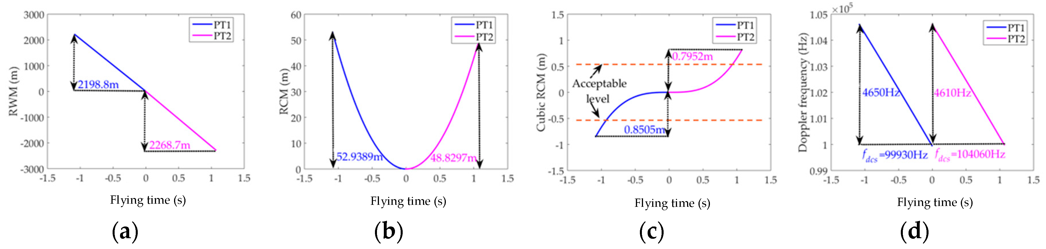
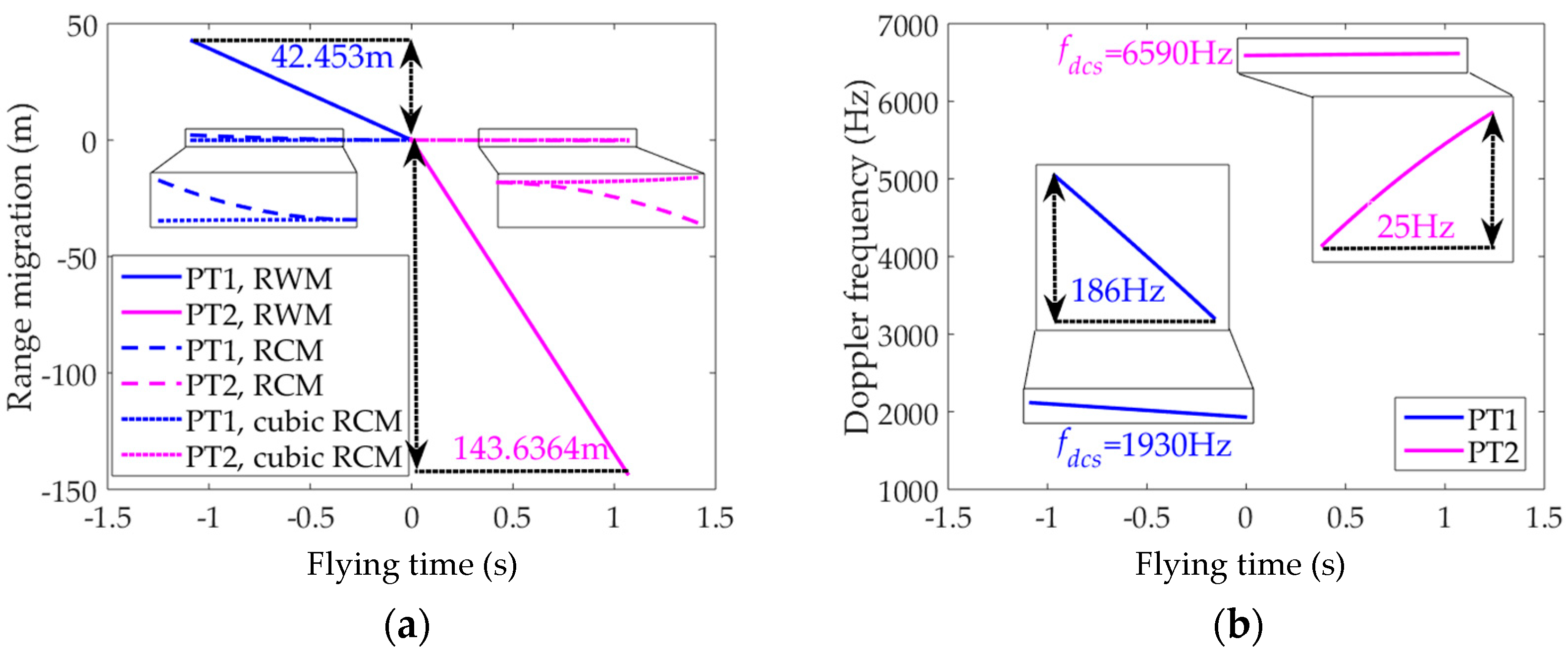
2.2.1. Range Migration

The range migration, which consist of the RWM, RCM, and high-order RCM, reflects the change in the instantaneous slant range of the signal. The range migration of NS-HSV-SAR differs from that of the traditional side-looking systems in two aspects, given the existence of the squint angle and high-speed movement of the radar platform. The first aspect is severe parameter coupling. A moving target is assumed to be located at the centre of the detected scene in a traditional case, and the RWM caused by the μ 1 term is mainly related to the radial velocity of the target [21]. However, the precise location of the target is constantly unknown in advance, and RWM is associated with the relative velocity and position between the target and the radar, as demonstrated in Appendix A, thus, they are coupled to each other. In terms of the RCM and cubic RCM caused by the μ 2 and μ 3 terms, the degree of their parameter coupling will only be increasingly serious, as presented in Appendix A. The second aspect is composed of the serious target energy diffusion and non-negligible high-order RCM. We illustrate the second aspect through a set of results simulated by the parameters listed in Table 1 for verification. Figure 3 exhibits the range migration results of PT1 and PT2 with the velocity of (−35, −35, 0) m/s. In Figure 3a–c, the range migration is particularly large that the target energy will be seriously smeared to thousands of range cells. The target is difficult to be imaged. Moreover, the cubic RCM is no longer ignored as in [24], even though our theory range resolution in this simulation (2.14 m) is not very high.

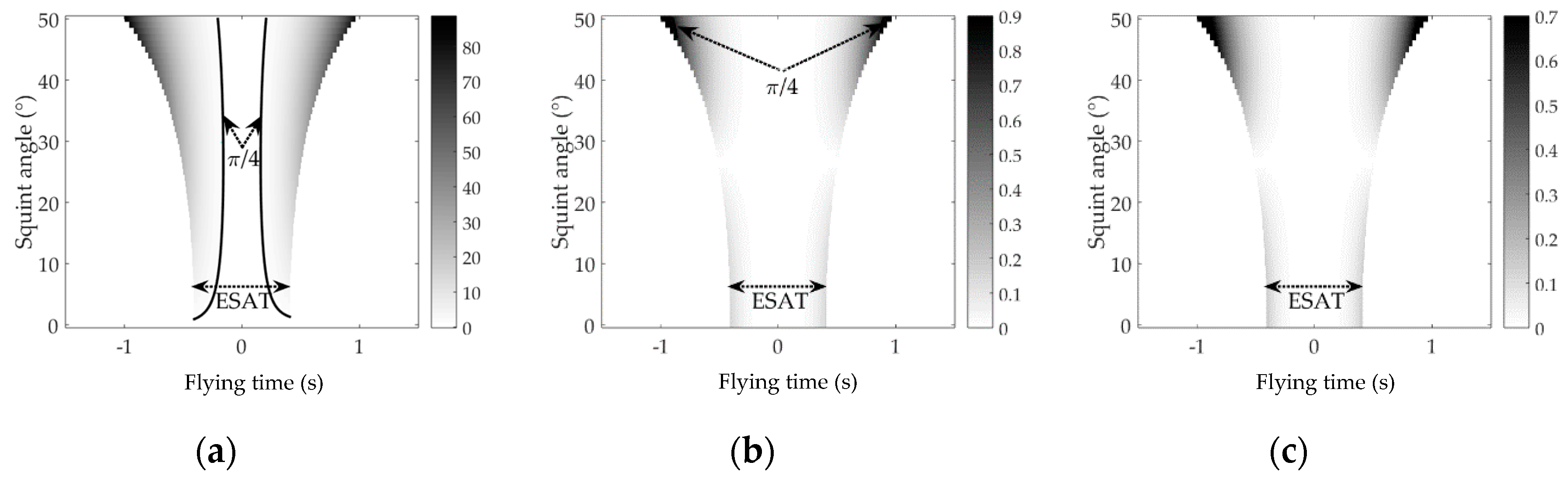
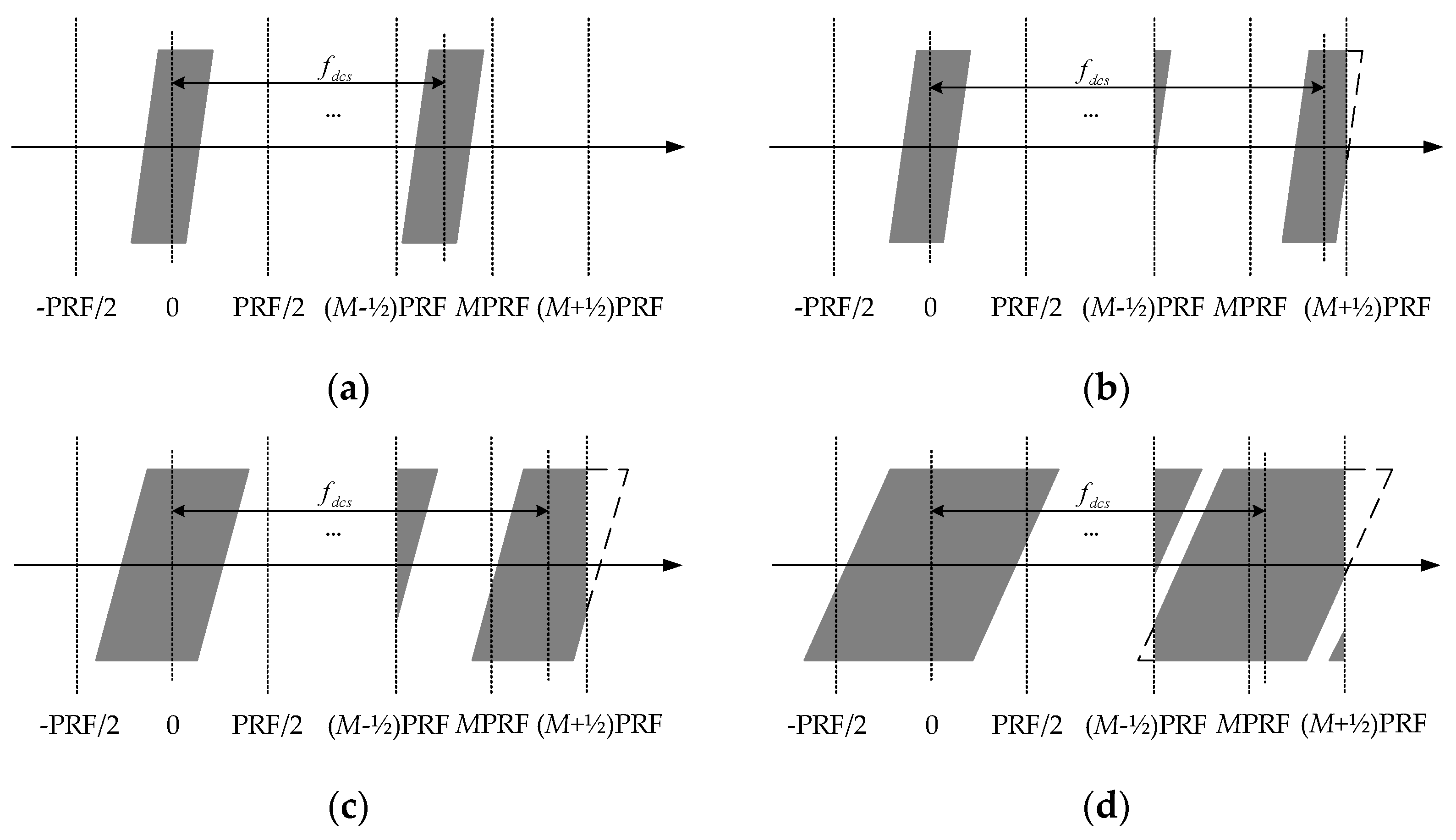
2.2.2. Azimuth Spectrum Distribution

The azimuth spectrum distribution of Equation (3) is mainly determined by its DFM, which includes the DCS f d c s and Doppler bandwidth B a z i :
f d c s = 2 f c μ 1 c
B a z i 2 f c c [ m a x ( 2 μ 2 η + 3 μ 3 η 2 ) m i n ( 2 μ 2 η + 3 μ 3 η 2 ) ]
where m a x ( ) and m i n ( ) represent the maximum and minimum operations, respectively. The main factors that affect the DFM are similar to those that influence the range migration. Therefore, the DCS will be severe, and the Doppler bandwidth will be large for the NS-HSV-SAR, similar to the range migration feature. Figure 3d depicts the DCS and Doppler bandwidth simulation results. Evidently, this result validates our conclusions. Given that the PRF for the NS-HSV-SAR is not high enough to avoid range ambiguity [30,31], the huge DCS and Doppler bandwidth can easily cause the Doppler ambiguity of the echo signal, thereby causing a false target imaging result by directly using matched filtering [10].
The Doppler ambiguity can be divided into two kinds. The first kind is Doppler centre blur caused by the DCS, which has been discussed in existing studies (e.g., [6,22,23]). This condition may introduce the following two types of azimuth spectrum distributions of the signal: spectrum in a PRF band and spanning neighbouring PRF, as displayed in Figure 4a,b, respectively. However, the Doppler bandwidth spanning caused by the high-order DFM (e.g., Figure 3d) must not be neglected for the squint-looking NS-HSV-SAR. This condition will cause another kind of Doppler ambiguity called Doppler spectrum ambiguity. Thus, two new complicated azimuth spectrum distributions, namely, Doppler bandwidths exceeding PRF and PRF/2 are derived in Figure 4c,d.
The abovementioned analyses can be verified by a set of 2-D spectrum simulations. The basic simulation parameters are listed in Table 1. A target located at the centre of the detected scene with a velocity of (8, 6, 0) m/s is selected as an example. Figure 5 illustrates the 2-D spectrum results for the different PRFs. The formats depicted in Figure 5a–c are consistent with the corresponding theoretical analysis demonstrated in Figure 4. In terms of the difference between Figure 4d and Figure 5d, the Doppler bandwidth is considerably larger than the PRF, thereby causing a serious Doppler spectrum ambiguity. Specifically, Figure 5d exhibits a general form of Figure 4d, i.e., the Doppler bandwidth exceeds several PRFs.

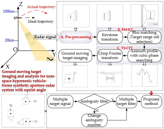
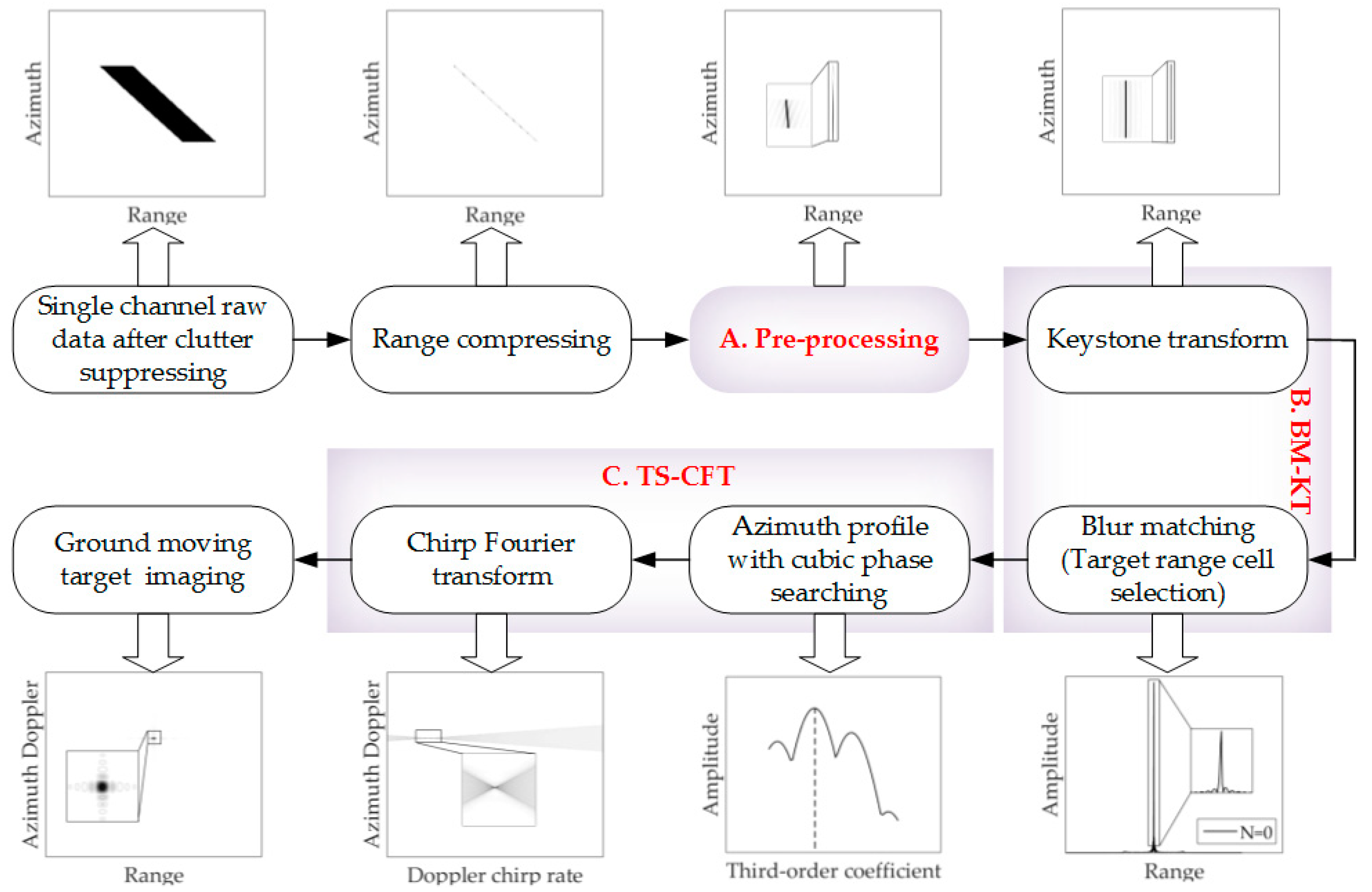
3. Proposed Algorithm Description

According to the description of the echo characteristics in the previous sections, for GMTIm, the three key issues, i.e. Doppler ambiguity, range migration, and azimuth focusing, must be considered in the signal processing of squint-looking NS-HSV-SAR. Thus, a new GMTIm algorithm is proposed in this section. The flowchart, corresponding subsections, and theoretical results of the proposed method are displayed in Figure 6. The three key steps of the proposed method, namely pre-processing, residual RWM correcting through BM-KT, and azimuth focusing through TS-CFT, have effectively solved the three abovementioned problems.

3.1. Pre-Processing

The GMTIm is essentially a 2-D match filtering for moving targets. For the distribution presented in Figure 4a, direct match filtering can effectively achieve target imaging. However, for the three other distributions illustrated in Figure 4, the presence of Doppler centre blur or spectrum ambiguity will trigger the direct match filtering to produce two or more target images. The PRF/2 spectrum shifting method [6,9,22] can eliminate the effect of Doppler centre blur depicted in Figure 4b, but this method completely fails in the case of Figure 4c,d, wherein the Doppler spectrum ambiguity existed. Traversal or searching is the most direct and effective means of resolving Doppler ambiguity [6,10,22], but the coexistence of Doppler centre blur and spectrum ambiguity leads to complex searching procedure. If the Doppler spectrum can be controlled within PRF/2 and the DCS is close to 0 Hz, then the probability of false targets focusing, and numerous searching times will be greatly considerably decreased. In [3,23,24], the deramp function is created to compress the spectrum, whereas the function parameters are difficult to be directly determined. By integrating the abovementioned important results, a pre-processing function based on the prior known information is created to diminish the effect of Doppler ambiguity and range migration in this section.
The pre-processing function primarily uses the existing prior known information to achieve the optimal possible Doppler spectrum compression and DCS, rather than obtain the precise target focusing similar to [3,23]. According to Equations (4) and (5), and Appendix A, the Doppler ambiguity and range migration are mainly induced by the movement of the NS-HSV-SAR, which is considerably faster than the target. Moreover, a narrow azimuth beam is typically used in the current SAR/GMTI system [30,31,32]. Thus, the pre-processing function can be expressed as:
H p r e ( f , η ) = exp [ j 4 π ( f + f c ) c ( μ 1 , p η + μ 2 , p η 2 + μ 3 , p η 3 ) ]
where f denotes the range frequency, and μ 1 , p , μ 2 , p , and μ 3 , p are expounded in Appendix A. After pre-processing, the echo signal in the range frequency and azimuth time domain can be denoted as:
s p r e ( f , η ) = f f t t [ s m f ( t , η ) ] H p r e ( f , η )
where f f t [ ] denotes a fast Fourier transform (FFT) operation along the dimension.
Figure 7 shows the residual range migration and DFM of PT1 and PT2 after pre-processing. Most range migrations have been corrected and the remaining part is mainly composed of RWM in Figure 7a. The DCS and Doppler bandwidth considerably decreased in Figure 7b in comparison with Figure 3d. According to the PRF selection strategy in [32,33], the azimuth spectrum distribution of PT1 and PT2 can only be one of those in Figure 4a or Figure 4b, wherein Figure 4a is most likely. The abovementioned results can be further promoted to other targets, which is discussed in Section 6.4.

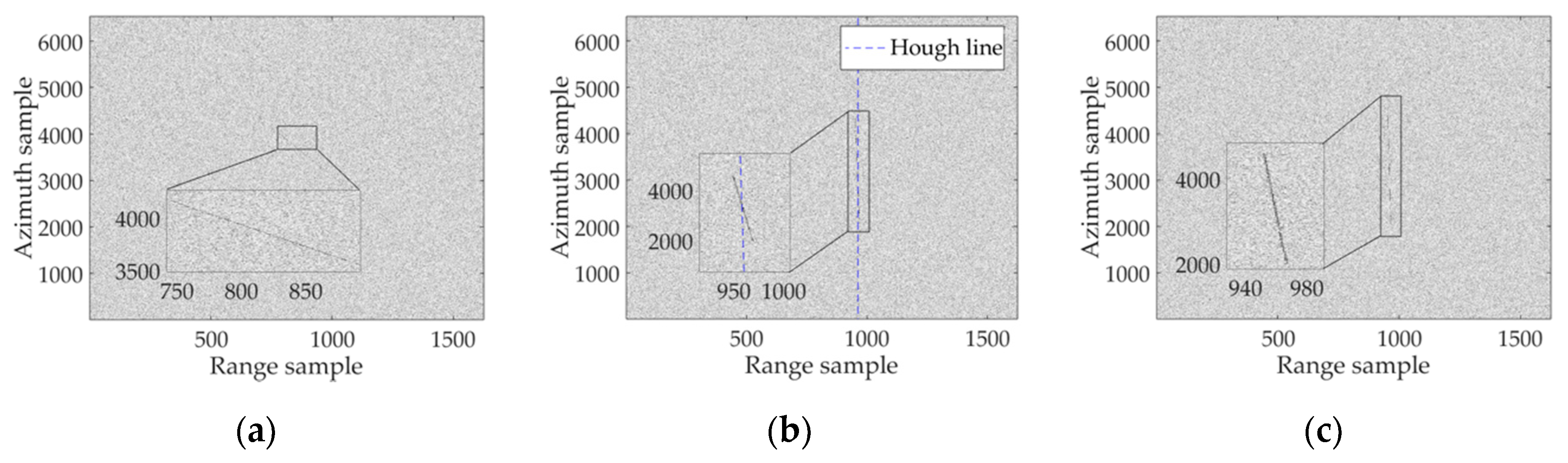
3.2. Residual RWM Correcting: BM-KT

The residual RWM can be corrected by Hough transform [6,24,25] or KT [7,22,23,24]. The KT can simultaneously achieve an RWM correction of different targets without any prior target information at a low SNR, in comparison with the Hough transform. However, the KT suffers from the Doppler centre blur problem [26]. The echo signal after pre-processing will probably have a Doppler centre blur, as analysed in Section 3.1. Thus, a BM-KT method is proposed here.
Considering that the echo is sampled by the PRF for a pulse radar, the signal in Equation (7) can be rewritten as:
s p r e ( f , η ) = exp [ j 4 π ( f + f c ) c ( μ 0 + μ ˜ 1 η + μ ˜ 2 η 2 + μ ˜ 3 η 3 ) ] exp [ j 2 π N × P R F ( f f c 1 ) η ]
where N is the ambiguity number of the Doppler centre blur, μ ˜ 1 = μ 1 μ 1 , p + N c × P R F 2 f c , μ ˜ 2 = μ 2 μ 2 , p , and μ ˜ 3 = μ 3 μ 3 , p . Then, after performing KT, we obtain:
s K T ( f , ζ ) = exp [ j 4 π f c c ( μ 0 + μ ˜ 1 ζ + μ ˜ 2 ζ 2 + μ ˜ 3 ζ 3 ) ] exp ( j 4 π f c μ 0 ) exp ( j 2 π f f + f c N × P R F × ζ )
where ζ denotes the new slow time variable. The derivation in Equation (9) is expounded in Appendix B. Evidently, the residual RWM still exists in the last item of Equation (9) given the existence of the Doppler centre blur. For illustration, several simulation results are presented in Figure 8 with a target located at (52,212, 34,791, 0) m. The target velocity is (−28, −23, 0) m/s. The simulation parameters are listed in Table 1 and the SNR is −15 dB. The range migration displayed in Figure 8b has been substantially corrected after pre-processing in comparison with the range compressed signal exhibited in Figure 8a. Although the target energy is accumulated at a certain degree, it is not considerably different from the noise background. The Hough line extracted by the Hough transform does not accurately match the residual RWM, as illustrated in Figure 8b. The KT has failed to corrected the residual RWM depicted in Figure 8c because the remaining DCS (3240 Hz) is larger than the PRF. A direct method for solving the KT inapplicability is to compress the last item of Equation (9) using:
H B M ( f , ζ ; N ) = exp ( j 2 π f f + f c N × P R F ζ )
where N is previously unknown, thereby making the direct obtainment of Equation (10) infeasible. However, the target velocity is limited to a certain known region [24], and the Doppler ambiguity number is an integer. Moreover, N has decreased into a small scope after pre-processing. The difficulty of the blur-matching step for Equation (10) will not considerably increase.
The image entropy value is used to determine N [23] but is sensitive to background noise. The simulated result displayed in Figure 8d confirmed that the differences in entropy values for different N are small, and the calculated outcome for N is incorrect. Considering that a radar signal is typically processed on the basis of the range cells, and the range dimension focusing can be obtained after a residual RWM correction, we can determine Equation (10) by blur matching, i.e., comparing the amplitude along a range for each N. In Figure 8e, only if N is matched, then the target energy can be focused on a range cell, such as the red solid line. Then, RWM can be corrected as Figure 8f after compensating Equation (9) by Equation (10) with the determined N. This approach also facilitates multiple target processing, which is discussed in Section 4.2.

3.3. Azimuth Focusing: TS-CFT

After performing BM-KT, the target is well-focused on a range dimension with sufficient SNR, and the azimuth focusing can be separately processed in each range cell. Then, the cumbersome process of tackling all range cells is prevented. The azimuth profile of a focused target can be written as:
s B M - K T ( μ 0 , ζ ) = exp [ j 4 π f c c ( μ 0 + μ ˜ 1 ζ + μ ˜ 2 ζ 2 + μ ˜ 3 ζ 3 ) ]
Equation (11) is a polynomial phase signal (PPS), and its coefficients are not particularly large after pre-processing. A popular approach to handling PPS is the CFT method [34]. However, CFT is effective for a quadratic chirp-type signal. Considering that Equation (11) is a cubic chirp-type signal, a compensating function is constructed to eliminate the cubic term:
H c u b i c ( t , ζ ; μ ˜ 3 ) = exp ( j 4 π f c c μ ˜ 3 ζ 3 )
where μ ˜ 3 is obtained using the following cost function:
μ ˜ ^ 3 = a r g m a x μ ˜ 3 | C F T ζ [ s B M - K T ( t , ζ ) H c u b i c ( t , ζ ; μ ˜ 3 ) ] |
where a r g m a x ( ) denotes the arguments of the maxima, and C F T ζ ( ) denotes CFT operation over ζ . Given that μ ˜ 2 denotes the remaining Doppler chirp rate, it can be obtained using the following equation:
μ ˜ ^ 2 = c 4 f c × a r g m a x γ a | C F T ζ [ s B M K T ( t , ζ ) H c u b i c ( t , ζ ; μ ˜ ^ 3 ) ] |
Then, the azimuth focusing function can be expressed as:
H a z i ( t , ζ ) = exp [ j 4 π f c c ( μ ˜ ^ 2 ζ 2 + μ ˜ ^ 3 ζ 3 ) ]
According to Equations (9), (10) and (15), the moving target can be focused on range time and azimuth Doppler domain:
s ( t , f ζ ) = f f t ζ [ s B M K T ( t , ζ ) H a z i ( t , ζ ) ]
where f ζ denotes the Doppler frequency variable.
The abovementioned procedure can be recognised as Fourier transform (FT) after the matching of the high-order DFM. The FT can be easily performed through the FFT, but the remaining parameters such as μ ˜ 2 and μ ˜ 3 in Equation (15) must be obtained. The scope and step-size of μ ˜ 2 and μ ˜ 3 are the key parameters in determining the traversal efficiency, wherein the former can be obtained through known traffic information, and the latter can be designed in advance through the demand for azimuth resolution.

3.3.1. Scope

The scope of μ ˜ 2 and μ ˜ 3 through monotonicity analysis is difficult to determine given the serious parameter coupling. However, the theory of SAR [20] denotes that the edge of the detection scene has a large DFM. Thus, the four edge points PT1, PT2, PT3, and PT4 presented in Figure 1 are firstly selected to calculate the traversal scope. Furthermore, the velocity of the target is a key factor that affects its value. The road position information (e.g., open street map) and the speed data (e.g., the legal maximum velocity in China for civilian vehicles in high way is 120 km/h) are utilised to determine the boundary velocity. Then, a small search scope can be obtained because using the existing traffic information can considerably improve the processing efficiency [35,36].

3.3.2. Step-Size

According to Equation (5) and azimuth resolution ρ a , the maximum step-size values for μ ˜ 2 and μ ˜ 3 can be calculated separately in accordance with the following inequalities:
| 4 f c c [ m a x ( Δ μ ˜ 2 ζ ) m i n ( Δ μ ˜ 2 ζ ) ] | ρ a 2
| 6 f c c [ m a x ( Δ μ ˜ 3 ζ 2 ) m i n ( Δ μ ˜ 3 ζ 2 ) ] | ρ a 2
where Δ μ ˜ i denotes the step-size of μ ˜ i .
For the sake of clarity, we present an example here on the basis of the parameters listed in Table 1 and target illustrated in Figure 8. The scopes of μ ˜ 2 and μ ˜ 3 are calculated as (−1, 1) and (−0.03, 0.03), respectively, on the basis of the abovementioned sections. These scopes are considerably smaller than an aimless traversal. In accordance with Equations (17) and (18), the step-size values of μ ˜ 2 and μ ˜ 3 are all approximately 0.001. For μ ˜ 3 , this step-size is acceptable, and the traversal number (i.e., 61) will not cause complexity, but for μ ˜ 2 , the traversal burden (i.e., 2001) of this step-size is unbearable. Thus, a large step-size (e.g., 0.01) can be utilised for rough traversal. Then, a small scope is obtained for an accurate traversal. The total traversal number for μ ˜ 2 will decrease by approximately 10-fold, i.e., 2001 to 262, using the abovementioned two-step approach. Figure 9 demonstrate several simulation results. After obtaining μ ˜ 3 in Figure 9a, μ ˜ 2 can be easily obtained in Figure 9b through two-step traversal. The substitution of μ ˜ 2 and μ ˜ 3 into Equation (15) indicates that the target can be focused by Equation (16), as depicted in Figure 13a. Notably, the scope of traversal can be further decreased by utilizing the road position information. A detailed discussion on using road information is presented in [35,36].

4. Implementation Considerations

4.1. Curvilinear Trajectory
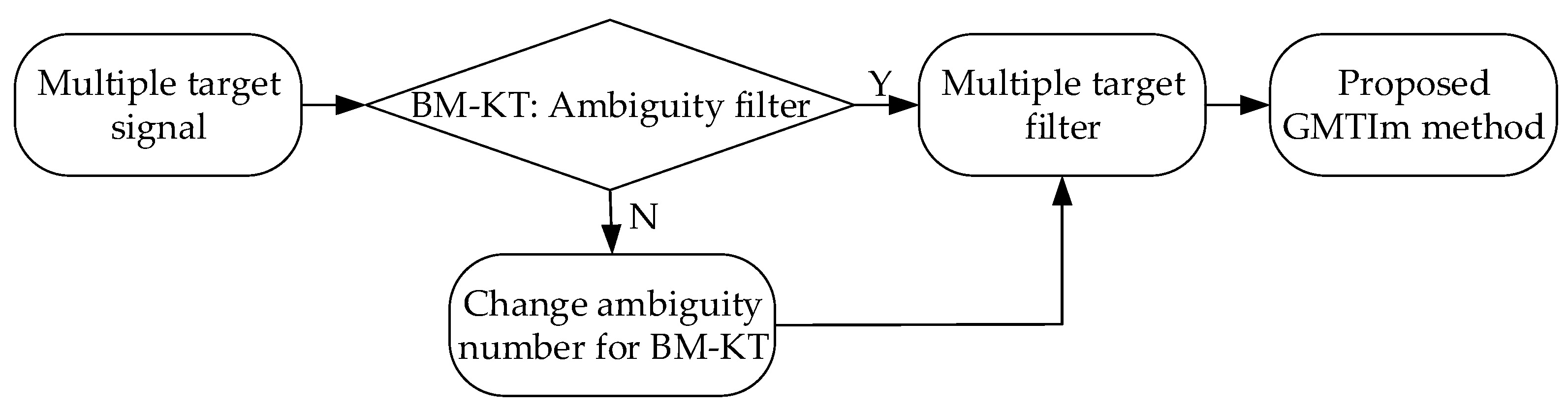
In practice, the NS-HSV-SAR platforms typically have a curvilinear trajectory, rather than the ideal linear trajectory [37]. In Figure 1, we can attribute the main cause of the curvilinear trajectory to the effect of acceleration a [38]. Then, Equation (1) can be rewritten as:
| R ( η ) | = | R 0 ( v v t ) η 1 2 a η 2 |
We can also perform the Taylor series expansion in Equation (19). The values and physical explanations of the ith order coefficient are derived in Appendix A. In previous sections, our GMTIm method is based on the third-order range model. However, the existence of acceleration does not guarantee the accuracy of the third-order range model. We must consider the high-order range model. Evidently, if the high-order ( i 4 ) term of the range model can be ignored before or after certain processing, the proposed GMTIm method can be used for curvilinear trajectory. Thus, the effect of the high-order terms on phase error, and spatial and velocity variations are analysed by using the parameters listed in Table 1. The exposure area of the NS-HSV-SAR is approximately 2.45 × 2.18 km2 (range × azimuth), and the along- and across-track velocity scopes of the target are all (−35, 35) m/s according to the analysis in Section 3.3. The definition of spatial variations for GMTIm is the same as that of the SAR stationary target imaging [39]. Moreover, the definition of velocity variation is that the slant range for any moving targets within the illuminated area of the radar can be approximated by that of the stationary target at the reference position.
The small acceleration case [38], e.g., a = ( 2.1 , 1.9 , 2 ) m/s2, is firstly analysed, as demonstrated in Figure 10. The phase errors caused by the μ 3 term with different target locations and velocities are considerably greater than the acceptable level π / 4 , as exhibited in Figure 10a,b. However, the phase errors of the μ 4 term displayed in Figure 10c,d are tolerable. Thus, the proposed method can be directly applied to a small acceleration case.
For the NS-HSV-SAR with strong manoeuvrability, e.g., a = ( 49 , 51 , 50 ) m/s2 [2,38], the analysis is depicted in Figure 11. We must analyse the phase errors caused by the μ 4 term with different target locations and velocities, as presented in Figure 11a,b, respectively, because the large acceleration exacerbates the phase error caused by the μ 3 term. Evidently, the phase error caused by the μ 4 term cannot be ignored. However, the simulation results illustrated in Figure 11c,d show that the spatial and velocity variations in the μ 4 term are negligible. We must directly compensate the high-order terms through the following improved pre-processing function to use our method under a large acceleration condition similar to Equation (6):
H i m p - p r e ( f , η ) = exp [ j 4 π ( f + f c ) c | R ref v η 1 2 a η 2 | ]

4.2. Multiple GMTIm

The validity of the proposed GMTIm method for a moving target is verified in Section 3. However, multiple targets may exist in a practical scene. Whether the proposed GMTIm method is suitable for this condition must be analysed. Firstly, the pre-processing function is not sensitive to the number of targets, because it is created on the basis of prior knowledge and not related to any target information. Secondly, the TS-CFT is suitable for multiple targets given the property of CFT, i.e., CFT can be used to match the multiple chirp rates in a chirp-type signal with multiple chirp components [34]. Thus, we must only illustrate the effectiveness of BM-KT to demonstrate that the proposed method can be used for multiple GMTIm.
In general, KT is a linear transform and can simultaneously correct RWM for all targets. However, the different targets may have a different Doppler centre blur (after pre-processing). This condition will affect the implementation of KT. The existence of Doppler centre blur will induce target energy diffusion after KT, as described in Section 3.2; otherwise, the target energy is focused on the range dimension. We can create an ambiguity filter [23], which will uniformly process targets with the same degree of Doppler centre blur, because the radar signal processing is performed on each range cell. Fortunately, the BM-KT can be recognised as such a filter as previously analysed.
Notably, the SNR of the target in the detected scene may also be different. The high SNR target will affect the performance of the low target. Thus, the targets’ imaging must be performed separately. Similar to our previous work [40], we designed a multiple target filter. The specific description of the filter can be found in Appendix C. Therefore, the proposed GMTIm method remains valid for multiple targets, and the entire procedure is plotted in Figure 12.

5. Experiment Results

We present three sets of numerical simulations in this section to validate the effectiveness of the proposed method. The first set was used for comparative analysis with the existing method. The second and the third sets were used to verify the multiple target imaging performances under the linear and curvilinear trajectory. Notably, all simulations were conducted after a clutter suppression [41,42], and the main NS-HSV-SAR system parameters are listed in Table 1.

5.1. Performance Comparison with Existing Methods

To the best of our knowledge, few studies on GMTIm for the NS-HSV-SAR are available, especially for the squint-looking geometry. However, in accordance with the classification of the existing algorithms in [6], our method can be categorised as a KT based technique. Therefore, several state-of-the-art KT based methods with few restrictions on application scenes or with similar scenarios were selected for comparison experiments, including the KT based descending stage method for side-looking NS-HSV-SAR [3], KT based long time coherent integration [22], and robust Deramp-Keystone methods [23]. We compared these methods with respect to performance and computational complexity.

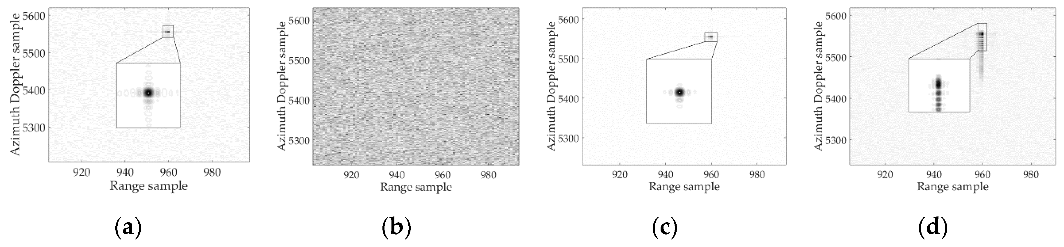
5.1.1. Focusing Performance

The target depicted in Figure 8 was selected as an example here. All simulation results are shown in Figure 13. In Figure 13a,c, the target can be well focused by the proposed method and the KT based long time coherent integration method [22], respectively, because the proposed method and the KT based long time coherent integration method [22] are based on the idea of traversal. By comparison, the imaging results of the KT based descending stage method [3] and the robust Deramp-Keystone method [23] are defocused in Figure 13b,d. For the KT based descending stage method [3], the target is seriously defocused in the entire 2-D plane because it does not consider the Doppler centre blur, thereby resulting in the inability of KT to directly correct the residual RWM. Moreover, although [3] has analysed the cubic phase item, the high-order DFM after the deramp can be ignored. Thus, the target is defocused in an azimuth Doppler dimension. For [23], the target is defocused in the azimuth dimension because it completes the range dimension focusing but ignores the residual high-order DFM.

5.1.2. Computational Complexity

The computational complexities of the abovementioned three methods and the proposed method for one moving target are summarised in Table 2. The computational complexity of range focusing is mainly concentrated on the ambiguity number traversal of the Doppler centre blur, because all these methods are based on KT. Evidently, the KT based descending stage method [3] does not have any traversal. For the KT based long time coherent integration method [22] and the robust Deramp-Keystone method [23], the maximum number of traversals is 2 × r o u n d [ | 2 f c μ 1 / ( c × P R F ) | ] + 3 , where r o u n d [ ] denotes the rounding operation. By comparison, the complexity of the proposed method decreased to 2 × r o u n d [ | 2 f c μ ˜ 1 / ( c × P R F ) | ] + 3 , where | μ ˜ 1 | < | μ 1 | because a pre-processing step with nearly no computational complexity is included in our method. We used the target exhibited in Figure 8 as an example for clarity purpose. The maximum traversal values for [22] and the robust Deramp-Keystone method [23] are 13, but the proposed method is only 5.
For azimuth focusing, the KT based long time coherent integration method [3] and the robust Deramp-Keystone method [23] are directly achieved by FFT with a small computational complexity. The computational complexity of [22] is about O ( M 2 M 3 N r N a l o g 2 N a ) , where M 2 and M 3 denote the searching time for c 2 and c 3 in [22], respectively, and N r and N a indicate the number of range and azimuth cells, respectively. By comparison, the target has been focused on a range dimension before azimuth focusing for our method. Thus, the total computational complexity of the proposed method is O ( M 2 M 3 N a l o g 2 N a ) , where M 2 and M 3 denote the searching times for μ ˜ 2 and μ ˜ 3 , respectively, and M 2 < M 2 and M 3 < M 3 due to pre-processing. Moreover, the computational complexity combined with the time-saving strategy proposed in Section 3.3 will only be small. The target presented in Figure 8 was used as an example; the computation burden in [22] is approximately 3.7866 × 10¹⁵, whereas that of the proposed method is approximately 1.0103 × 10¹⁰. When the proposed time-saving strategy is adopted, the computational complexity of the proposed method decreases to 1.0199 × 10⁹.
In summary, although the KT based descending stage method [3] and the robust Deramp-Keystone method [23] have a low computational complexity, their performances cannot be effectively guaranteed. The proposed method has a similar performance as the KT based long time coherent integration method [22], but the amount of computation is decreased considerably.

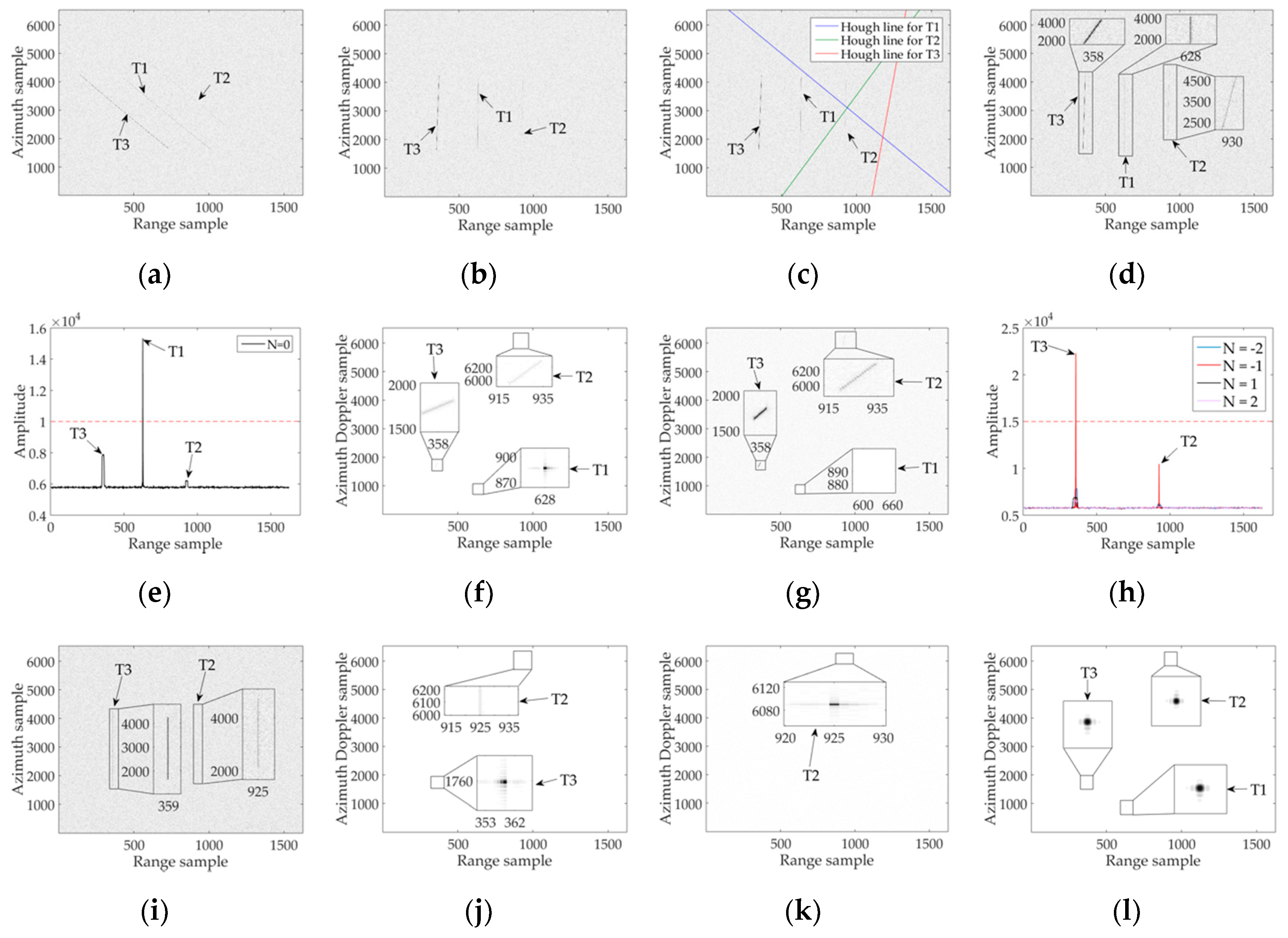
5.2. Multiple Target Imaging under a Linear Trajectory Case

Three targets with different Doppler centre blur and SNR were used to verify the performance of the proposed method under the linear trajectory case for multiple target imaging. The specific target parameters are listed in Table 3, and the simulation results are illustrated in Figure 14.
In Figure 14a, the range migration after range compress is large enough that the target energy smeared among multiple range cells. After pre-processing using Equation (6) in Figure 14b, the range migration of the targets is considerably decreased, and is mainly composed of RWM. Moreover, the azimuth spectrum distributions for all targets changed after pre-processing, as analysed in Section 3.1. The DCS and Doppler bandwidth before and after pre-processing are listed in Table 4. The Doppler spectrum ambiguity for all targets are eliminated in comparison with the system PRF, but the Doppler centre blur with the ambiguity number of −1 are still exists for T2 and T3 after pre-processing.
After pre-processing, the residual RWM must be corrected. The Hough transform [24] failed to extract the Hough lines in Figure 14c because the target energy remains spanning over multiple range and azimuth cells and a strong noise background. Therefore, the compensation function created by the Hough line cannot effectively correct RWM. By comparison, the BM-KT was used to correct the residual RWM of unambiguity T1 depicted in Figure 14d. Although the initial SNR of T1 was not the highest among the three targets, the range profile demonstrated in Figure 14e shows that the concentration of energy on range dimension makes it easier to be imaged. After using the proposed TS-CFT, T1 is well focused in Figure 14f. Since the residual RWM of T2 and T3 still existed, they are all unfocused in Figure 14f. According to the multiple target process flowchart exhibited in Figure 12, T1 is separated from the mixed signal displayed in Figure 14f using the proposed multiple target filter, and T2 and T3 are focused on a range dimension through the proposed BM-KT. The corresponding simulation results are presented in Figure 14g–i. Notably, the unambiguity target has been focused, and the remaining targets show a Doppler centre blur. This condition can prevent the duplication work of searching N = 0 in Figure 14h. T3 is firstly focused on in Figure 14j through the proposed method, because the SNR is larger in T3 than in T2; this result can also be found in Figure 14h. Then, the weakest target T2 is extracted and focused on in Figure 14k on the basis of the multiple target process flowchart illustrated in Figure 12. Finally, we can obtain the final imaging for multiple targets by merging all the focused results demonstrated in Figure 14l.

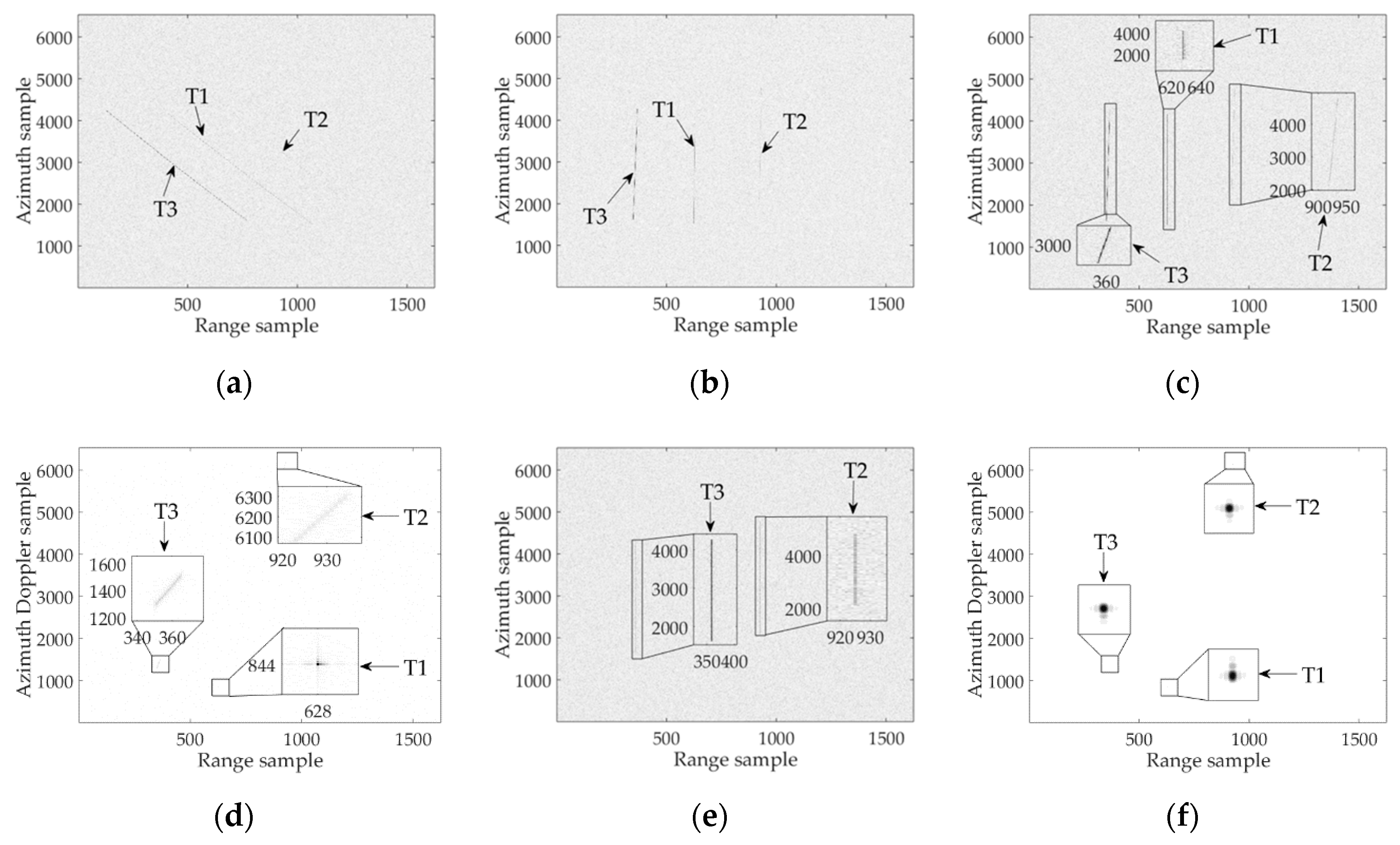
5.3. Multiple Target Imaging under a Curvilinear Trajectory Case

In this section, the simulation results were used for the targets in Table 3 to validate the performance of the proposed method under the curvilinear trajectory case for multiple target imaging. In Figure 15a, the range migrations after range compression are large enough that the target energy smeared among multiple range cells. The acceleration we used in our simulations is sufficiently large. Thus, the pre-processing step was performed using Equation (20) in accordance with the analysis in Section 4.1. Figure 15b depicts the pre-processing result. The range migrations of the targets considerably decrease and mainly comprise the RWM. The DCS and Doppler bandwidth before and after pre-processing are listed in Table 5. The Doppler spectrum ambiguity for all targets was eliminated, but the residual RWMs of T2 and T3 still cannot be directly corrected by the KT exhibited in Figure 15c in comparison with the system PRF because the Doppler centre blur still existed in T2 and T3, and the remaining ambiguity number for T2 and T3 is −1. Thus, T1 is imaged in Figure 15d. According to the multiple target process flowchart in Figure 12, T1 is separated from the mixed signal presented in Figure 15d using the proposed multiple target filter, and T2 and T3 are focused on the range dimension through the proposed BM-KT, as illustrated in Figure 15e. The final imaging is obtained in Figure 15f for multiple targets under the curvilinear trajectory case by merging the GMTIm results.

6. Discussion

Generally, no method is applicable to all conditions. Here, we present several preliminary discussions on the applicability and limitation of the proposed GMTIm method from five aspects.

6.1. Clutter Effect

An effective clutter suppression is a crucial prerequisite for achieving accurate GMTIm. The residual strong clutter will inevitably affect the imaging performance of the target. This condition challenges the signal-to-clutter-ratio (SCR) after clutter suppression. Generally, a peak sidelobe ratio (PLSR) denotes the amplitude ratio between the maximum sidelobe and the mainlobe. To ensure that the target is not submerged by the residual clutter sidelobe, the output SCR ( S C R o u t ) after a clutter suppression can be evidently determined by the PLSR. The theoretical PSL for a well-focused image is −13 dB [20]. Thus, we obtain S C R o u t 13 dB.
Many excellent clutter suppression methods, such as space-time adaptive processing (STAP) [41] and displaced phase centre antenna (DPCA) [42], have been proposed. The performance of the clutter suppression is evaluated using the improvement factor (IF) [41]:
I F = S C R o u t S C R i n
where S C R i n denotes the input SCR before clutter suppression. The IF of the clutter suppression method must satisfy I F 13 dB in a practice scene because most clutter suppression techniques are derived on the basis of ensuring the target energy. For most detection scenarios, STAP and DPCA have been verified to satisfy this requirement [3,41,42]. However, for extremely heterogeneous scenarios or non-ideal data acquisition conditions, additional effective clutter suppression methods must be designed and applied. Considering that the main work of this study is GMTIm, we assume that clutter suppression can be performed by utilizing the STAP or DPCA, as mentioned in many GMTIm studies (e.g., [7,8,9,21,22,23,24] and the references therein). The study of clutter suppression and GMTIm methods that are suitable for extremely heterogeneous scenarios and non-ideal data acquisition conditions will be investigated in the future.

6.2. Wavelength Effect

Fundamentally, the accuracy of SAR processing is relative to the radar wavelength. The signal model with limited orders will encounter problems eventually if the wavelength decreases. However, according to several published results [31,32,43,44,45], the NS-HSV-SAR has certain restrictions on selecting of wavelength. In practice, the plasma sheath generated by the high-speed movement of the radar platform in near-space affects the propagation of electromagnetic waves [43,45]. The choice of wavelength is crucial for the attenuation and reflection of the transmitting signal. Simulation results in [44] show that a short wavelength typically causes low attenuation, however, selecting a particularly short wavelength for the NS-HSV-SAR at present is impractical considering the application requirement and overall system design (e.g., load space, transmit power, and beam width). Thus, the traditional SAR that uses X-band (0.025–0.0375 m) and Ku-band (0.016–0.028 m) are advised to be selected. Our proposed method will be suitable for most situations because a short wave length (0.02 m) in the Ku-band is adopted to analyse the signal model in this study.

6.3. Resolution Effect

Resolution is another key factor that affects the accuracy of SAR signal processing. High-resolution [46] or very high-resolution [47] SAR imaging technology for stationary targets have drawn considerable attention and achieved many outstanding results. However, excessively high resolution is unsuitable for NS-HSV-SAR GMTIm at present. Firstly, a narrower transmitting bandwidth (which leads to a low range resolution) makes the dispersion effect caused by plasma sheath small [44]. Secondly, a high resolution intensifies the range migration and DFM of the target, thereby affecting the target detection probability. Thus, a medium resolution (2.14 m) with 70 MHz transmitting bandwidth is selected in this study by integrating the parameter setting strategy for GMTIm in the current studies or systems [20,21,22,23,24,25,26,35,43,44]. For future high- and very high-resolution cases (e.g., decimetres or millimetres level), the range migration and DFM caused by the high order terms in Equation (2) are intolerable. The approximations of pre-processing and BM-KT in the proposed method require further consideration.

6.4. Removal of Doppler Spectrum Ambiguity

Considering the coexistence of Doppler centre blur and spectrum ambiguity for the NS-HSV-SAR, we created a pre-processing function to eliminate the effect of the latter. However, for the sake of clarity, only one target is used as an example to illustrate the effectiveness of the proposed function in Section 3.1. In this section, a set of analyses about the precision of the removal of the Doppler spectrum ambiguity are depicted in Figure 16. The maximum Doppler bandwidth after pre-processing does not exceed 500 Hz, regardless of the targets in different positions exhibited in Figure 16a or varying velocities displayed in Figure 16b. A large acceleration was used in our simulations. The pre-processed Doppler bandwidth will only be small for a small acceleration or no acceleration case because acceleration will lead to Doppler bandwidth expansion [38]. Thus, if the PRF of the radar system is between 1000 and 3000 Hz, then the proposed pre-processing function can be well performed. This parameter selection is theoretically feasible [30,31,32,33]. Notably, a large acceleration will occur with the development of technology and application requirement; this phenomenon is beyond the scope of this study.

6.5. Efficiency Improvement

For practical application, the efficiency of the proposed method must be further improved. The computational complexity of the proposed method is mainly reflected in the BM-KT and TS-CFT for multiple targets. A minimal Doppler centre blur (approximately 3~5 times) search for BM-KT after pre-processing is tolerable [22,23]. Moreover, every blur matching can be performed on the target with the same degree of ambiguity. Furthermore, various methods, e.g., Chirp-Z transform [48] and scaled FFT [49], can be used to solve the complexity caused by the interpolation of KT. The complexity of TS-CFT is mainly caused by the specific implementation of CFT. However, a time-saving strategy is proposed in Section 3.3, and the discrete FT based method, such as fast discrete quadratic phase transform [50], is available and can effectively improve the efficiency of CFT.

7. Conclusions

This paper focuses on GMTIm and analysis for a squint-looking NS-HSV-SAR. A precise range model is firstly utilized on the basis of the phase error analysis considering the complex range history, parameter coupling, and Doppler ambiguity of the echo signal. Then, all potential distributions of echo’s azimuth spectrum are derived, and a GMTIm method is proposed in accordance with the detailed analysis of the signal characteristics. The properties of the proposed GMTIm method are as follows: considers the simultaneous existence of the Doppler centre blur and spectrum ambiguity; convenient unified process of range focusing for multiple targets without any target knowledge; and the TS-CFT method suitable for the cubic chirp-type signal with a low complexity searching strategy. The implementation considerations, including the generalisation of the proposed method for the NS-HSV-SAR with a curvilinear trajectory, implementation of the proposed method for multiple target imaging, and applicability and limitation of the proposed method, are also discussed. Validity and performance were investigated through theoretical analysis and numerical experiments.
However, clutter suppression is not fully considered in this method, and the target indication in the BM-KT is the direct use of amplitude detection. The proposed method does not consider the existence of interference in practice. Besides, this paper mainly considers GMTIm and disregards target parameter estimation and relocation. Furthermore, the target is focused on range time and azimuth Doppler frequency domain through the proposed method. Although this result is suitable for professionals to analyse the characteristics of the targets in different dimensions, this result cannot intuitively facilitate the radar operator in obtaining the target position and motion information as range time and azimuth time domain. The abovementioned problems will be investigated in the future.

Author Contributions

Conceptualization, Z.C. and L.Z.; Data curation, Z.C. and Y.Z.; Formal analysis, Z.C., C.L. and Y.H.; Funding acquisition, Y.Z., L.Z. and S.T.; Investigation, Z.C. and S.T.; Methodology, Z.C. and C.L.; Project administration, Y.Z. and L.Z.; Supervision, L.Z.; Validation, Z.C., Y.Z. and C.L.; Writing—original draft, Z.C.; and Writing—review and editing, Y.Z., L.Z., C.L., Y.H. and S.T.

Funding

This research was funded by the National Natural Science Foundation of China, grant numbers 61871305, 61671361, 61601343, and 61731023; by the National Natural Science Foundation of Shaanxi Province, grant number 2018JM6054; and the APC was funded by the National Natural Science Foundation of China, grant number 61871305.

Conflicts of Interest

The authors declare no conflict of interest.

Appendix A

In this appendix, the values and physical explanations of the ith order coefficient μ i for linear and curvilinear trajectories are derived correspondingly. The linear case can essentially be regarded as a curvilinear trajectory when a = 0 . Thus, in this appendix, Equation (19) is used as an example for derivation.
Generally, Equation (19) can be rewritten as:
| R ( η ) | = [ R 0 ( v v t ) η 1 2 a η 2 ] , [ R 0 ( v v t ) η 1 2 a η 2 ] = | R 0 | 2 2 R 0 , ( v v t ) η R 0 , a η 2 + | v v t | 2 η 2 + ( v v t ) , a η 3 + 1 4 | a | 2 η 4
where denotes the inner product operation. Considering that μ i is derived by Taylor series expansion, the Taylor series is expressed as:
| R ( η ) | = + 1 i ! d i | R ( η ) | d η i | η = 0 η i
where d i f ( x ) d x i denotes the ith order derivative of f ( x ) with respect to x . In accordance with Equations (A2) and (2), we have:
μ i = 1 i ! d i | R ( η ) | d η i | η = 0
For the sake of clarity, the values of μ i are all listed in Table A1. Evidently, the Doppler modulation rate and high-order terms vary with a . This condition results in more complex signal characteristics than the linear trajectory analysed in Section 4.1. Moreover, the coupling between the parameters becomes increasingly serious with the increase in order.
Table A1. Values and physical explanation for the ith order coefficient with different trajectories.
μ i Value (Linear)Value (Curvilinear)Physical Explanation
μ 0 | R 0 | | R 0 | Initial slant range
μ 1 ( v v t ) , R 0 / μ 0 ( v v t ) , R 0 / μ 0 Relative radial velocity
μ 2 ( | v v t | 2 μ 1 2 ) / ( 2 μ 0 ) ( | v v t | 2 R 0 , a μ 1 2 ) / ( 2 μ 0 ) Relative radial acceleration
μ 3 μ 2 μ 1 / μ 0 [ ( v v t ) , a 2 μ 2 μ 1 ] / ( 2 μ 0 ) Relative radial jerk
μ 4 ( μ 2 2 + 2 μ 3 μ 1 ) / ( 48 μ 0 ) ( | a | 2 4 μ 2 2 8 μ 3 μ 1 ) / ( 192 μ 0 ) Relative fourth-order radial acceleration
Considering that the stationary target at the centre of the detected scene has been adopted to aid in developing the pre-processing function, in accordance with Table A1 and Equation (A3), μ 1 , p , μ 2 , p , and μ 3 , p can be denoted as:
μ 1 , p = v , R ref | R ref |
μ 2 , p = | v | 2 μ 1 , p 2 2 | R ref |
μ 3 , p = μ 2 , p μ 1 , p | R ref |

Appendix B

In this appendix, the derivation of Equation (9) is expounded.
The transform kernel of KT is denoted as:
( f + f c ) η = f ζ
The substitution of Equation (A7) into Equation (8) yields:
s K T ( f , ζ ) = exp [ j 4 π ( f + f c ) c μ 0 ] exp ( j 4 π f c c μ ˜ 1 ζ ) exp [ j 4 π f c 2 c ( f + f c ) μ ˜ 2 ζ 2 ] × exp [ j 4 π f c 3 c ( f + f c ) 2 μ ˜ 3 ζ 3 ] exp ( j 2 π f f + f c N P R F ζ )
Certain approximations can be utilised because f < f c is satisfied for the SAR/GMTI systems:
f c f + f c 1 f f c   and   f c 2 ( f + f c ) 2 1 2 f f c
The substitution of Equation (A9) into Equation (A8) yields:
s K T ( f , ζ ) = exp [ j 4 π λ ( μ 0 + μ ˜ 1 ζ + μ ˜ 2 ζ 2 + μ ˜ 3 ζ 3 ) ] exp [ j 4 π f c ( μ 0 + μ ˜ 2 ζ 2 + 2 μ ˜ 3 ζ 3 ) ] × exp ( j 2 π f f + f c N × P R F ζ )
Figure A1. Residual RCM after KT with acceleration: (a) moving target with different locations; and (b) moving target with different velocities.
Remotesensing 10 01966 g0a1
In Equation (A10), the cubic RCM becomes twice the original, and the RCM still exists. However, the cubic RCM and RCM depicted in Figure A1 are sufficiently small, and the maximum value of the total RCM does not exceed two range cells for different locations and velocities of moving targets, and even our simulation acceleration is adequately large. This slight spanning of the RCM slightly affects the diffusion of the target energy, which has been verified in [51]. Thus, Equation (A10) can be simplified as Equation (9).

Appendix C

In this appendix, the multiple target filter is expounded.
For simplicity, two targets are used as an example:
s ( t , ζ ) = s 1 ( t , ζ ; R 1 ) + s 2 ( t , ζ ; R 2 )
where s i ( t , ζ ; R i ) is the ith target echo with a slant range R i .
In general, different targets correspond to various initial slant ranges and Doppler frequencies. The performance of the proposed GMTIm method for the first target yields:
s ( R , f ζ ) = s 1 ( R 1 , f ζ , 1 ) + s 2 ( R 2 , η ) H i m a g e ( s 1 )
where denotes the focus procedure, and H i m a g e ( s 1 ) represents the proposed GMTIm function for the first target. The first target is focused on range time and Doppler frequency domain, whereas the second target is only focused on range dimension and smears along the Doppler dimension. The first target can be separated from the mixed signal in Equation (A12) by filtering the aforementioned formula with a 2-D band-stop filter centred at the position of the first target. Then, the second target can be obtained by the inverse-process of Equation (A12) in accordance with H i m a g e ( s 1 ) . Similarly, we can iteratively repeat the abovementioned procedure for multiple targets.

References

  1. Wang, W.Q. Near-space vehicles: Supply a gap between satellites and airplanes. IEEE Aerosp. Electron. Syst. Mag. 2011, 25, 4–9. [Google Scholar] [CrossRef]
  2. Wang, W.Q. Near-Space Remote Sensing: Potential and Challenges; Springer: New York, NY, USA, 2011. [Google Scholar]
  3. Wang, Y.; Cao, Y.; Peng, Z.; Su, H. Clutter suppression and moving target imaging approach for multichannel hypersonic vehicle borne radar. Digit. Signal Process. 2017, 68, 81–92. [Google Scholar] [CrossRef]
  4. Wang, Y.; Cao, Y.; Peng, Z.; Su, H. Clutter suppression and GMTI for hypersonic vehicle borne SAR system with MIMO antenna. IET Signal Process. 2017, 11, 909–915. [Google Scholar] [CrossRef]
  5. Jao, J.K. Theory of synthetic aperture radar imaging of a moving target. IEEE Trans. Geosci. Remote Sens. 2001, 39, 1984–1992. [Google Scholar] [Green Version]
  6. Huang, P.; Liao, G.; Yang, Z.; Xia, X.G.; Ma, J.; Zheng, J. Ground maneuvering target imaging and high-order motion parameter estimation based on second-order keystone and generalized Hough-HAF transform. IEEE Trans. Geosci. Remote Sens. 2017, 55, 320–335. [Google Scholar] [CrossRef]
  7. Perry, R.P.; Dipietro, R.C.; Fante, R.L. SAR imaging of moving targets. IEEE Trans. Aerosp. Electron. Syst. 1999, 35, 188–200. [Google Scholar] [CrossRef]
  8. Kirkland, D. Imaging moving targets using the second-order keystone transform. IET Radar Sonar Navig. 2011, 5, 902–910. [Google Scholar] [CrossRef]
  9. Zhu, S.; Liao, G.; Qu, Y.; Zhou, Z.; Liu, X. Ground moving targets imaging algorithm for synthetic aperture radar. IEEE Trans. Geosci. Remote Sens. 2011, 49, 462–477. [Google Scholar] [CrossRef]
  10. Zhu, S.; Liao, G.; Yang, D.; Tao, H. A new method for radar high-speed maneuvering weak target 726 detection and imaging. IEEE Geosci. Remote Sens. Lett. 2014, 11, 1175–1179. [Google Scholar]
  11. Xu, J.; Yu, J.; Peng, Y.; Xia, X.G. Radon–Fourier transform for radar target detection, I: Generalized Doppler filter bank. IEEE Trans. Aerosp. Electron. Syst. 2011, 47, 1186–1202. [Google Scholar] [CrossRef]
  12. Xu, J.; Xia, X.G.; Peng, S.; Yu, J.; Peng, Y.; Qian, L. Radar maneuvering target motion estimation based on generalized Radon–Fourier transform. IEEE Trans. Signal Process. 2012, 60, 6190–6201. [Google Scholar]
  13. Zeng, H.; Chen, J.; Wang, P.; Yang, W.; Liu, W. 2-D coherent integration processing and detecting of 736 aircrafts using GNSS-based passive radar. Remote Sens. 2018, 10, 1164. [Google Scholar] [CrossRef]
  14. Chen, V.C.; Ling, H. Joint time–frequency analysis for radar signal and image processing. IEEE Trans. Signal Process. Mag. 1999, 16, 81–93. [Google Scholar] [CrossRef]
  15. Tang, S.; Zhang, L.; Guo, P.; Liu, G.; Zhang, Y.; Li, Q.; Gu, Y.; Lin, C. Processing of monostatic SAR with general configurations. IEEE Trans. Geosci. Remote Sens. 2015, 53, 6529–6546. [Google Scholar] [CrossRef]
  16. Xiong, B.; Xu, J.; Peng, S.; Yang, J. Ground moving targets signal modeling for multi-channel squint-looking SAR. In Proceedings of the International Radar Conference, Xi’an, China, 14–16 April 2013; pp. 1–7. [Google Scholar]
  17. Jing, K.; Xu, J.; Huang, Z.; Yao, D.; Long, T. GMTI for squint looking XTI-SAR with rotatable forward-looking array. Sensors 2016, 16, 873. [Google Scholar] [CrossRef] [PubMed]
  18. Garren, D.A. Signature morphology effects of squint angle for arbitrarily moving surface targets in spotlight synthetic aperture radar. IEEE Trans. Geosci. Remote Sens. 2015, 53, 6241–6251. [Google Scholar] [CrossRef]
  19. Garber, W.; Pierson, W.; Meginnis, R.; Majumder, U.; Minardi, M.; Sobota, D. Performance evaluation of SAR/GMTI algorithms. Proc. SPIE. 2016, 9843, 1–14. [Google Scholar]
  20. Cumming, I.G.; Wong, F.H. Digital Processing of Synthetic Aperture Radar Data: Algorithm and Implementation; Artech House: Norwood, MA, USA, 2005. [Google Scholar]
  21. Yang, J.; Liu, C.; Wang, Y. Imaging and parameter estimation of fast-moving targets with signle-antenna SAR. IEEE Geosci. Remote Sens. Lett. 2014, 11, 529–533. [Google Scholar] [CrossRef]
  22. Huang, P.; Liao, G.; Yang, Z.; Xia, X.G.; Ma, J.; Ma, J. Long-time coherent integration for weak maneuvering target detection and high-order motion parameter estimation based on keystone transform. IEEE Trans. Signal Process. 2016, 64, 4013–4026. [Google Scholar] [CrossRef]
  23. Sun, G.; Xing, M.; Xia, X.G.; Wu, Y.; Bao, Z. Robust ground moving-target imaging using deramp-keystone processing. IEEE Trans. Geosci. Remote Sens. 2013, 51, 966–982. [Google Scholar] [CrossRef]
  24. Yang, J.; Zhang, Y. An airborne SAR moving target imaging and motion parameters estimation algorithm with azimuth-dechirping and the second-order keystone transform applied. IEEE J. Sel. Top. Appl. Earth Observ. Remote Sens. 2015, 8, 3967–3976. [Google Scholar] [CrossRef]
  25. Yang, J.; Liu, C.; Wang, Y. Detection and imaging of ground moving targets with real SAR data. IEEE Trans. Geosci. Remote Sens. 2015, 53, 920–932. [Google Scholar] [CrossRef]
  26. Yang, J.; Huang, X.; Jin, T.; Thompson, J.; Zhou, Z. New approach for SAR imaging of ground moving targets based on a Keystone transform. IEEE Geosci. Remote Sens. Lett. 2011, 8, 829–833. [Google Scholar]
  27. Tang, S.; Zhang, L.; So, H.C. Focusing high-resolution highly-squinted airborne SAR data with maneuvers. Remote Sens. 2018, 10, 862. [Google Scholar] [CrossRef]
  28. Lin, C.; Tang, S.; Zhang, L.; Guo, P. Focusing high-resolution airborne SAR with topography variations using an extended BPA based on a time/frequency rotation principle. Remote Sens. 2018, 10, 1275. [Google Scholar] [CrossRef]
  29. Robinson, P.N. Depth of field for SAR with aircraft acceleration. IEEE Trans. Aerosp. Electron. Syst. 1984, 20, 603–616. [Google Scholar] [CrossRef]
  30. Wang, W.Q. Near-space vehicle-borne SAR with reflector antenna for high-resolution and wide-swath remote sensing. IEEE Trans. Geosci. Remote Sens. 2012, 50, 338–348. [Google Scholar] [CrossRef]
  31. Davis, M.E. Quest for a simultaneous SAR/GMTI waveform. In Proceedings of the IEEE Radar Conference, Monterey, CA, USA, 11–14 September 2013; pp. 134–139. [Google Scholar]
  32. Liu, X.; Zhou, P.; Zhang, X.; Sun, W.; Dai, Y. The parameter design results of near space airship SAR system. In Proceedings of the IEEE International Geoscience and Remoting Sensing Symposium, Beijing, China, 10–15 July 2016; pp. 1102–1105. [Google Scholar]
  33. Shu, Y.; Liao, G.; Yang, Z. Design considerations of PRF for optimizing GMTI performance in azimuth multichannel SAR systems with HRWS imaging capability. IEEE Trans. Geosci. Remote Sens. 2014, 52, 2048–2063. [Google Scholar]
  34. Xia, X.G. Discrete Chirp-Fourier transform and its application to chirp rate estimation. IEEE Trans. Signal Process. 2000, 48, 3122–3133. [Google Scholar]
  35. Baumgartner, S.V.; Krieger, G. Fast GMTI algorithm for traffic monitoring based on a priori knowledge. IEEE Trans. Geosci. Remote Sens. 2012, 50, 4626–4641. [Google Scholar] [CrossRef] [Green Version]
  36. Guerci, J.R.; Baranoski, E.J. Knowledge-aided adaptive radar at DARPA: An overview. IEEE Signal Process. Mag. 2006, 1, 41–50. [Google Scholar] [CrossRef]
  37. Carter, P.H., II; Pines, D.J.; Rudd, L.V. Approximate performance of periodichy-personic cruise trajectories for global reach. IBM J. Res. Dev. 2000, 44, 703–714. [Google Scholar] [CrossRef]
  38. Tang, S.; Zhang, L.; Guo, P.; Liu, G.; Sun, G. Acceleration model analyses and imaging algorithm for highly squinted airborne spotlight-mode SAR with maneuvers. IEEE J. Sel. Topics Appl. Earth Observ. Remote Sens. 2015, 8, 1120–1131. [Google Scholar] [CrossRef]
  39. Tang, S.; Lin, C.; Zhou, Y.; So, H.C.; Zhang, L.; Liu, Z. Processing of long integration time spaceborne SAR data with curved orbit. IEEE Trans. Geosci. Remote Sens. 2018, 56, 888–904. [Google Scholar] [CrossRef]
  40. Zhou, Y.; Chen, Z.; Zhang, L.; Xiao, J. Micro-Doppler curves extraction and parameters estimation for cone-shaped target with occlusion effect. IEEE Sens. J. 2018, 18, 2892–2902. [Google Scholar] [CrossRef]
  41. Ward, J. Space Time Adaptive Processing for Airborne Radar; Technical Report; MIT Lincoln Laboratory: Lexington, MA, USA, 1994; p. 1015. [Google Scholar]
  42. Maori, D.C.; Sikaneta, I. A generalization of DPCA processing for multichannel SAR/GMTI radars. IEEE Trans. Geosci. Remote Sens. 2013, 51, 560–572. [Google Scholar] [CrossRef]
  43. Wang, R.; Wang, X.; Cheng, S.; Meng, Y.; Zhang, G.; Zhou, Y. Plasma passive jamming for SAR based on the resonant absorption effect. IEEE Trans. Plasma Sci. 2018, 46, 928–933. [Google Scholar] [CrossRef]
  44. Li, N. Research on Availability and Algorithm of Hypersonic Missile-Borne Bistatic SAR. Ph.D. Thesis, Graduate School of National University of Defense Technology, Changsha, China, 2011. [Google Scholar]
  45. Kennel, C.F. The propagation of electromagnetic waves in plasmas. Proc. IEEE 1965, 53, 2168. [Google Scholar] [CrossRef]
  46. Moreira, A.; Prats-Iraola, P.; Younis, M.; Krieger, G.; Hajnsek, I.; Papathanassiou, K.P. A tutorial on SAR. IEEE Geosci. Remote Sens. Mag. 2013, 5, 6–43. [Google Scholar] [CrossRef] [Green Version]
  47. Reigber, A.; Scheiber, R.; Jäger, M.; Prats-Iraola, P.; Hajnsek, I.; Jagdhuber, T.; Papathanassiou, K.; Nannini, M.; Aguilera, E.; Baumgartner, S.; et al. Very-high-resolution airborne synthetic aperture radar imaging: Signal processing and applications. Proc. IEEE 2013, 101, 759–783. [Google Scholar] [CrossRef]
  48. Lanari, R. A new method for the compensation of the SAR range cell migration based on the chirp z-transform. IEEE Trans. Aerosp. Electron. Syst. 1995, 31, 1296–1299. [Google Scholar] [CrossRef]
  49. Natroshvili, K.; Loffeld, O.; Maya, A.; Ortiz, M.; Knedlik, S. Focusing of general bistatic SAR configuration data with 2-D inverse scaled FFT. IEEE Trans. Geosci. Remote Sens. 2006, 44, 2718–2727. [Google Scholar] [CrossRef]
  50. Ikram, M.Z.; Meraim, K.A.; Hua, Y. Fast quadratic phase tranform for estimating the parameters of multicomponent chirp signals. Digit. Signal Process. 1997, 7, 127–135. [Google Scholar] [CrossRef]
  51. Su, J.; Xing, M.; Wang, G.; Bao, Z. High-speed multi-target detection with narrowband radar. IET Radar Sonar Navig. 2010, 4, 595–603. [Google Scholar] [CrossRef]
Figure 1. Geometrical model of a squint-looking NS-HSV-SAR and moving target.
Remotesensing 10 01966 g001
Figure 2. Phase errors for different range models: (a) second-order model; (b) third-order model; and (c) fourth-order model.
Remotesensing 10 01966 g002
Figure 3. Simulated results for range migration and Doppler frequency migration: (a) Range walk migration; (b) Range curvature migration; (c) Cubic RCM; and (d) Doppler centre shift and Doppler bandwidth.
Remotesensing 10 01966 g003
Figure 4. Theoretical azimuth spectrum distributions: (a) spectrum entirely in a PRF band; (b) spectrum spanning neighbouring PRF; (c) Doppler bandwidth exceeding PRF/2; and (d) Doppler bandwidth exceeding the PRF.
Remotesensing 10 01966 g004
Figure 5. Simulated 2-D spectrum with different PRF for one moving target: (a) PRF = 17,000 Hz; (b) PRF = 13,000 Hz; (c) PRF = 6000 Hz; and (d) PRF = 800 Hz.
Remotesensing 10 01966 g005
Figure 6. Flowchart of the proposed algorithm and corresponding subsections and theoretical results for a moving target.
Remotesensing 10 01966 g006
Figure 7. Simulated results for pre-processing: (a) remaining range migration; and (b) remaining DFM.
Remotesensing 10 01966 g007
Figure 8. Simulation results for Hough transform, KT and BM-KT: (a) range compressed signal; (b) pre-processing and Hough transform result; (c) KT result; (d) image entropy result for each N; (e) blur matched result for each N; and (f) BM-KT result.
Remotesensing 10 01966 g008aRemotesensing 10 01966 g008b
Figure 9. Simulation results for the proposed TS-CFT: (a) traversal result for μ ˜ 3 ; and (b) rough and accurate traversal results for μ ˜ 2 .
Remotesensing 10 01966 g009
Figure 10. Effects of the μ 3 and μ 4 terms on phase errors with small acceleration. The unit of the contour maps is π / 4 : (a) phase error of the μ3 term with different target locations; (b) phase error of the μ3 term with different target velocities; (c) phase error of the μ4 term with different target locations; and (d) phase error of the μ4 term with different target velocities.
Remotesensing 10 01966 g010
Figure 11. Effects of the μ 4 terms on phase error, and spatial and velocity variations with large acceleration. The unit of the contour maps is π / 4 : (a) phase error of the μ 4 term with different target locations; (b) phase error of the μ 4 term with different target velocities; (c) spatial variation of the μ 4 term; and (d) velocity variation of the μ 4 term.
Remotesensing 10 01966 g011
Figure 12. Flowchart of the proposed GMTIm method for handling multiple targets.
Remotesensing 10 01966 g012
Figure 13. Focusing performance comparison: (a) the proposed method; (b) the KT based descending stage method [3]; (c) the KT based long time coherent integration method [22]; and (d) the robust Deramp-Keystone method [23].
Remotesensing 10 01966 g013
Figure 14. Simulation results for multiple target imaging under the linear trajectory condition: (a) range compressed signal; (b) pre-processing result; (c) Hough transform result; (d) BM-KT result for T1; (e) range profile for Figure 15d; (f) imaging result for T1; (g) multiple target filter result for separating T1; (h) blur matching result for T2 and T3; (i) BM-KT for T2 and T3; (j) imaging result for T3; (k) imaging result for T2; and (l) multiple target imaging result.
Remotesensing 10 01966 g014
Figure 15. Simulation results for multiple target imaging under curvilinear trajectory condition: (a) range compressed signal; (b) pre-processing result; (c) BM-KT result for T1; (d) imaging result for T1; (e) multiple target filter result for separating T1 and BM-KT result for T2 and T3; and (f) multiple target imaging result.
Remotesensing 10 01966 g015
Figure 16. Remaining bandwidth after pre-processing with the acceleration of a = ( 50 , 50 , 50 ) m/s2: (a) moving target with different locations; and (b) moving target with different velocities.
Remotesensing 10 01966 g016
Table 1. Basic simulation parameters.
ParameterValueParameterValue
Carrier frequency14.7 GHzPRF2400 Hz
Pulse duration3 μsRadar position(0, 0, 30) km
Transmit bandwidth70 MHz v (linear)(0, 2000, 0) m/s
Squint angle30° v (curvilinear)(200, 2000, 200) m/s
Elevation angle60° a (curvilinear)(−50, −50, −50) m/s2
Table 2. Computational burden comparison.
MethodKTAzimuth Focusing
Proposed 2 × r o u n d [ | 2 f c μ ˜ 1 / ( c × P R F ) | ] + 3 O ( M 2 M 3 N a l o g 2 N a )
KT based descending stage method [3]//
KT based long time coherent integration method [22] 2 × r o u n d [ | 2 f c μ 1 / ( c × P R F ) | ] + 3 O ( M 2 M 3 N r N a l o g 2 N a )
robust Deramp-Keystone method [23] 2 × r o u n d [ | 2 f c μ 1 / ( c × P R F ) | ] + 3 /
Table 3. Moving target parameters for Section 5.2 and Section 5.3.
TargetInitial PositionVelocitySNR
T1(51,802, 34,221, 0) m(4, −3, 0) m/s−10 dB
T2(52,092, 34,851, 0) m(12, 16, 0) m/s−15 dB
T3(51,282, 34,041, 0) m(18, 22, 0) m/s−5 dB
Table 4. DCS and bandwidth for moving targets.
TargetDCS before Pre-ProcessingDCS after Pre-ProcessingBandwidth before Pre-ProcessingBandwidth after Pre-Processing
T197,125.6 Hz−874.4 Hz4627.5 Hz67.4 Hz
T296,638.5 Hz−1361.5 Hz4593.6 Hz69.6 Hz
T395,047.1 Hz−2952.9 Hz4586.3 Hz11.6 Hz
Table 5. DCS and bandwidth for moving targets.
TargetDCS before Pre-ProcessingDCS after Pre-ProcessingBandwidth before Pre-ProcessingBandwidth after Pre-Processing
T1103,322 Hz−891 Hz8984 Hz43 Hz
T2102,869 Hz−1344 Hz9006 Hz61 Hz
T3101,138 Hz−3075 Hz8896 Hz38 Hz

