Article

2D Frequency Domain Fully Focused SAR Processing for High PRF Radar Altimeters

1
Department of Electrical and Information Engineering, Politecnico di Bari, 70125 Bari, Italy
2
Aresys srl, via Flumendosa 16, 20132 Milan, Italy
*
Author to whom correspondence should be addressed.
Remote Sens. 2018, 10(12), 1943; https://doi.org/10.3390/rs10121943
Submission received: 27 August 2018 / Revised: 29 November 2018 / Accepted: 30 November 2018 / Published: 3 December 2018
(This article belongs to the Special Issue Advances in Satellite Altimetry and Its Application)

Abstract

:
Fully-focusing of radar altimeters is a recent concept that has been introduced to allow further improvement of along-track resolution in high pulse repetition frequency (PRF) radar altimeters. The straight potentiality of this new perspective reflects into a more accurate estimation of geophysical parameters in some applications such as sea-ice observation. However, as documented in a recent paper, such capability leaves unsolved the problem of the high computational effort required. In this paper, we face the problem of adapting for altimeters the Omega-Kappa SAR focusing algorithm that is performed in the two-dimensional wavenumber domain, accounting for the difference existing between SAR and altimeter from geometry (looking and swath width) and instrument (echoes are deramped onboard on receiving) point of view. Simulations and an application using in-orbit data show the effectiveness of the proposed approach and the highly reduced computational effort.

1. Introduction

During the last 20 years, a new paradigm for radar altimeter instruments has been designed, implemented, and exploited to observe the ocean and ice environment involving an accurate estimate of the range of the sensor above the Earth surface. High pulse repetition frequency (PRF) altimeter instruments are able to transmit pulses at a high pulse repetition frequency simultaneously guaranteeing their coherence [1]. Such instruments allow to exploit the Delay/Doppler (D/D) processing concept [2,3], which, by coherent summation of pulses within a burst, achieves an improvement in terms of along-track resolution and of Equivalent Number of Looks (ENL) compared to conventional pulse-limited altimeters. High PRF altimeters are currently exploited in operational missions, such as CryoSat [4] and Sentinel-3 [5], and are foreseen to be on board in forthcoming missions, such as Sentinel-6 [6]. From the applications point of view, high PRF altimeters in conjunction with D/D processing have improved the measurements of floating ice [7], land ice [4,8], ocean surface [9,10], coastal zone [11], and inland water [12].
While in D/D processing the coherent summation of pulses is performed over a limited number of successive pulses (i.e., bursts), the concept of coherent summation has recently been extended to the whole synthetic aperture. This is the so-called fully-focused (FF) concept [13,14], in which the different bursts within the antenna extent are coherently summed after phase compensation to increase the along-track resolution up to its theoretical limit (half the along-track antenna length). Coherent summation within the antenna aperture furtherly improves also the ENL with respect to D/D. In particular, in Reference [14], the potentiality of the FF processing was demonstrated using a focusing algorithm based on the back projection (BP), but the problem of its high computational effort was not addressed.
In this paper, by using a nadir-looking synthetic aperture radar (SAR) instrument [15], a high PRF altimeter, as we address the problem of revising and adapting the frequency domain Omega-Kappa (WK) focusing algorithm for SAR [16,17] to high PRF altimeters. Some adaptations are needed to account for the difference existing between the SAR and altimeter sensors in terms of geometry (looking and swath width) and instrument. The proposed method is a valid scheme for both closed-burst, such as in CryoSat, and open-burst acquisition modes, such as in Sentinel-6. The proposed algorithm has been proven to focus a point target with accuracy comparable to that of the algorithm in Reference [14] while sensibly reducing the computational burden, as necessary if the FF processing were to be operationally exploited in a forthcoming altimetry mission.
The remainder of the paper is organized as follows. In Section 2, the system is described and the unfocused impulse response function (IRF) is presented. Subsequently, the two-dimensional (2D) exact transfer function (ETF) of the unfocused IRF is derived. In Section 3, the ETF is used to derive the focusing algorithm in the 2D wavenumber domain (the so called WK-focusing). In Section 4, practical considerations about focusing and its implementation are provided. Finally, in Section 5, results about the quality and efficiency of the processing scheme on both simulated and real dataset are shown and discussed.

2. Context and Problem Statement

In order to adapt the 2D frequency domain SAR focusing scheme to high PRF altimeters, it is necessary to identify the main differences and similarities existing between the two systems. A first difference is the acquisition geometry, detailed in the following subsection for the altimeter case.
A difference between SAR and current altimeter sensors is represented by the instrument on-board receiving chain. For a large part of operative SAR sensors, the received signal is acquired, downconverted in frequency, sampled, and digitized. Range compression follows on ground by matched filtering. In the case of high PRF altimeters currently used in operations, instead, the receiving chain is based on deramp-on-receive, which consists in an analog mixing (multiplication) of the received echo with the replica of the transmitted pulse and a successive low-pass filtering and digitization. Across-track compression is achieved on ground by a Fourier transform. It is noteworthy, however, that in some cases deramping has been implemented also for SAR, as in the frequency modulated continuous wave (FMCW) SAR [18]. Likewise, the future Poseidon-4 altimeter instrument will be based on an on-board matched filter.
It can be noticed that for both systems the IRF is range-variant [3,16]. This means that it is not possible to make an exact focusing of the whole swath by a single compensation of the ETF on a data block in the double-transformed domain, since, in theory, the ETF is exact for a single slant range position only. In SAR, the data block is usually partitioned in different range strips and a different ETF is used to focus each range strip. In the Omega-Kappa algorithm [16] the final accuracy of the focused IRF is a function of the width of the range strips. In the case of altimeters, the extent of the receiving window in the across-track direction is very small compared to the sensor-target distance (around 60 m compared to an average altitude of 700 km for Cryosat). For this reason, the compensation performed by using a single ETF is reasonably accurate enough for the whole extent of the window. However, the central frequency used for altimeters is usually higher than that used by SAR sensors (as a typical example, the C-band Sentinel-1 carrier frequency is less than half of the Ku-band carrier adopted in Cryosat). This means that even a small phase contribution such as the delay due to the Doppler effect cannot be neglected, since it may induce mislocation of the focused target and/or blurring (i.e., defocusing).
The differences above justify the complete reformulation of the 2D transfer function for the altimeter, based on the stationary phase principle (SPP) approximation, on which the WK concept is based.

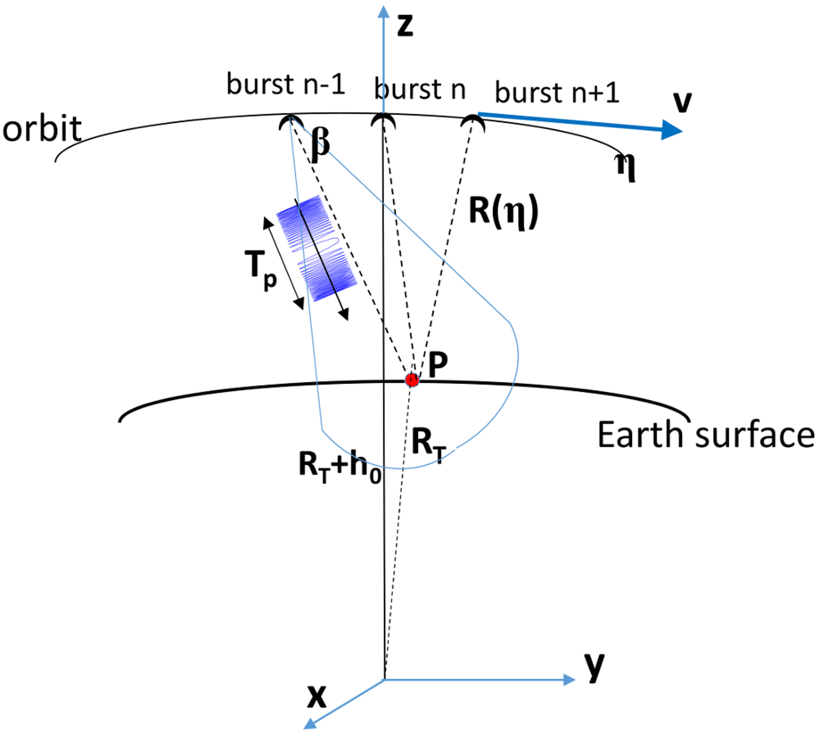
2.1. Acquisition Geometry

In Figure 1, the closed-burst timeline is considered.
Without loss of generality, we focus our attention on a limited observation time T o b s . The along-track time, η, is 0 in the middle of T o b s . When the sensor is at η = 0, the axis going from the Earth center to the sensor is the z-axis; the y-axis is perpendicular to the z-axis and on the same plane of the sensor velocity at η = 0; the x-axis completes the counter-clockwise triplet. To make simpler the notation, we also suppose that the along-track time η = 0 corresponds to the center of an emitted burst. To determine the ETF, the following simplifications are assumed:
  • The Earth is locally spherical of radius RT and fixed (i.e., not rotating);
  • The satellite orbit is locally circular and the satellite height h0 is locally constant;
  • The sensor speed v is constant;
  • As a consequence, the tracker value R t k r (i.e., an approximate estimation that the altimeter performs to evaluate the aperture time of the receiving window) is constant along the observation time;
  • The sensor attitude is nominal, i.e., the triplet {yaw, pitch, roll} are zero along the observation time;
  • In the derivation of the unfocused IRF, the monostatic approximation is used (i.e., the sensor transmits and receives at the same nominal position);
  • In this description, radiometry is not accounted for, nor thermal noise is included.
The system and geometric parameters used below are summarized in Table 1.

2.2. Unfocused IRF

Since an altimeter is a linear system, we can limit our description to a single point target on ground that is uniquely described by its range-to-target history   R ( η , t ) as a function of the fast time t and slow time η . Using the previous assumptions and according to the geometry of Figure 1 and a literature description, the unfocused IRF is:
h ( η , t ; R t k r ) A ( η ) G ( ϑ , β ) · e x p { j 2 π [ f c τ ( α ( 1 Δ ) τ f D ) t + α 2 τ 2 + Θ r ] }
β = c o s 1 ( R y z · S | R y z | | S | ) ,   ϑ = c o s 1 ( R x z · S | R x z | | S | )
where R y z is the projection of the sensor-target vector onto the YZ plane, R x z is the projection of the sensor-target vector onto the XZ plane, S is the sensor position, and all the vectors are function of the along-track time η . In the previous equation, τ = τ τ t k r = 2 c R ( η , t ) τ t k r , where τ t k r is the reference delay, τ t k r = 2 / c · R t k r . The received echo is a function of the along- and across-track target position, as well as of the reference tracker. The Doppler shift, a consequence of the continuous motion of the platform during the transmission and reception of the chirp, cannot be neglected due to the high carrier frequency. The resulting Doppler coefficient Δ (see Table 1) is a function of the radial speed that changes during the observation interval, and assumes very low values (e.g., Δ 10−6 using parameters from Table 1). For this reason, both the phase term Θ r = α Δ ( 1 Δ / 2 ) τ 2 and the correction ( 1 Δ ) applied to the frequency of the complex sinusoid can be neglected [13]. The only relevant term due to the centroid that cannot be ignored is the frequency shift f D ( η ) = Δ · f c , since it varies up to 16 kHz in a synthetic aperture of about T i l l 2 s (using parameters from Table 1). The amplitude is a function with two terms: (i) the radar equation term A ( η ) , which is a function of the sensor-target distance, the emitted power, and the atmospheric attenuation [19], and is a slowly varying contribution and can be omitted, as it can often be approximated to a constant; (ii) the antenna pattern term G ( ϑ , β ) , which is a function of the antenna along and across-track shape. The antenna term cannot be neglected, since the altimeter is designed to provide half the maximum directivity at the border of the illumination time. The antenna pattern is considered separable in the across- and along-track directions, respectively, so that we have G ( ϑ , β ) G c r ( ϑ ( r 0 ) ) G a l ( β ( η η 0 ) ) , being r 0 = R ( η 0 ) the across-track target distance and η 0 the instant of minimum sensor-target approach.
Considering the simplifications detailed above, the unfocused IRF results in
h ( η , t ; R t k r ) G c r ( r 0 ) G a l ( η η 0 ) · e x p { j 2 π [ f c τ ( α τ f D ) t + α 2 τ 2 ] }
We can decompose the phase of h ( η , t ; R t k r ) in three terms. The term e x p { j 2 π ( α τ f D ) t } is the range cell migration term and accounts for the variation in the sensor-target distance through τ . The term e x p { j π α τ 2 } , called residual video phase (RVP) in Reference [13], is the term with major difference w.r.t. the SAR impulse response, since it comes after the on-board deramping, a step commonly not performed by SAR instruments (an exception is the SPOTlight SAR [20]). The last term e x p { j 2 π f c τ } is the phase rotation due to delay. This term, called relative range phase (RRP), is the dominant phase term Reference [14].

2.3. Determination of 2D ETF

In principle, the 2D ETF is achieved by a double Fourier transform of Equation (2) after range compression. In the altimeter case, the across-track (i.e., range) compression is an inverse Fourier transform, since part of the compression has been already performed on board through deramping. For this reason, the 2D Fourier transform of the altimeter results in a direct along-track transform only:
H ( f a ,   t ; R t k r ) = η f a { h ( η , t ; R t k r ) } = = + G a l ( η η 0 ) · e x p { j 2 π [ f c τ ( α τ f D ) t + α 2 τ 2 ] } · e x p { j 2 π f a η } d η
where the across-track antenna term G c r ( r 0 ) was dropped to simplify the notation. It is important here to remark that this is the expression of the 2D ETF in the double-transformed frequency domain after range compression.
The integral in Equation (3) is extended in the entire along-track domain, although the antenna shape limits the integration interval. The previous expression is traditionally solved in the SAR literature by resorting to theStationary Phase Approximation (SPA) [21], a well-known result of differential calculus. The SPA states that, in case of integrals of the kind
I = + G ( x ) · e x p { j Φ t o t ( x ) } d x = G ( x ) · e x p { j [ Φ ( x ) k x x ] } d x
where the function G ( x ) is slowly changing with x , the solution can be approximated by using the following expression:
I G ( x ) π 2 π | Φ t o t ( x 0 ) | · exp { j [ Φ ( x 0 ) k x x 0 + π / 4 ] }
where x 0 is the stationary phase point (SPP), i.e., a value in x for which the first derivative of the whole phase is null: d [ Φ t o t ( x ) ] d x | x 0 = 0 .
In Equation (5), we take x = v e q η ,   k x = 2 π v e q f a and Φ ( x ) = 2 π [ f c τ ( α τ f D ) t + α 2 τ 2 ] for the current case. The equivalent speed v e q is a function of the orbit curvature: v e q = v / α T , with α T = ( R T + h 0 ) / R T . Moreover, the obliquity factor, i.e., the term 1 π 2 π | Φ t o t ( x 0 ) | · exp { j π / 4 } , is safely ignored in SAR systems, since it is almost a constant throughout the whole data block. An explicit expression of the integral in Equation (5) for the altimeter case is then (use also Equation (18) in Reference [15]):
H ( f a ,   t ; R t k r ) G a l ( f a F M ( t ) ) · e x p { j [ 2 π [ f c τ ( x 0 ) ( α τ ( x 0 ) f D ) t + α 2 τ ( x 0 ) 2 ] k x x 0 ] }
where F M ( t ) is the Doppler rate [14], i.e., the derivative of the instantaneous Doppler frequency, which is a function of the fast time.
To identify the SPP, d [ Φ t o t ( x ) ] d x | x 0 = 0 is to be solved. The first derivative of Φ t o t ( x ) , after some algebra, results in
d Φ t o t ( x ) d x = 2 π 2 c ( f c α t ) d δ R ( x ) d x + 2 π d f D ( x ) d x t + 8 π α c 2 δ R ( x ) · d δ R ( x ) d x k x
In case of circular orbit, a closed-form expression can be found for the stationary point x 0 . In this case, the sensor-target distance can be written by using the well-known SAR hodograph expression [15]: δ R ( x ) = R t k r 2 + x 2 R t k r . The problem to solve is, in this case, the following:
d Φ t o t ( x ) d x = [ 2 π 2 c ( f c α t ) 8 π α c 2 R t k r ] · x R t k r 2 + x 2 [ k x 2 π β t 8 π α c 2 x ] = 0
where β d f D ( x ) d x (it has been experimentally verified that the Doppler frequency can be optimally approximated by means of a line). Properly rearranged, the expression in Equation (8) is a fourth-order polynomial, the coefficients of which are a function of the sensor-target distance R , the slope of the Doppler frequency β , and the along-track wavenumber k x .
In the case when the circular orbit approximation cannot be hold, it is necessary to fit the trend of the relative sensor-target distance for the along-track times corresponding to the current data block by using a third- or fourth-order polynomial: δ R ( x ) = p ( 4 ) ( x ) . The same approximation can be used to get the trend of the Doppler frequency with the along-track distance, i.e., f D ( x ) . In this case, Equation (7) does not result in a closed-form expression but it is still possible to solve for the stationary point by resorting to any method to find the zero of a function.
In principle, once the stationary point has been evaluated, the focused IRF is exact only at that slant range (the phase Φ ( x ) is a function of τ = 2 c R ( η , t ) τ t k r , i.e., of the distance between sensor and target). Moreover, in the case of a noncircular orbit, for which the numerical approximation of the sensor-target distance is along-track dependent, the solution for x 0 is also along-track dependent. In traditional SAR processing, the computation of the ETF for each on-ground position is unfeasible and the stationary point is usually evaluated at the center of range strips narrow enough and an azimuth block not longer than one synthetic aperture. In the altimeter case, however, due to the reduced number of raw data samples in fast time, it could be manageable to solve d [ Φ t o t ( x ) ] d x | x 0 = 0 for each point of a data block in   ( k x , t ) coordinates. Alternatively, x 0 can be evaluated on a coarser grid and interpolating the WK focusing operator in the remaining positions. We verified that the second approach is faster and does not threaten the accuracy of the final results.

2.4. Unfocused IRF and ETF for Closed-Burst Acquisition

In a closed-burst acquisition, the echoes from the target are not continuously received. The burst-by-burst acquisition can be modelled on the unfocused IRF as follows:
h c b ( η , t ; R t k r ) = h ( η , t ; R t k r ) · n T i l l r e c t ( η n / B R F N a z / P R F )
Since in Reference [14] the authors already derived the 2D ETF for a scanning SAR, it is possible to adopt the same results, achieving the 2D ETF for a closed-burst high PRF altimeter:
H c b ( f a , t ; R t k r ) G a l ( f a F M ( t ) ) · k r e c t ( f a + k · W p + F M · η 0 W B ) ·
e x p { j [ 2 π [ f c τ ( x 0 ) ( α τ ( x 0 ) f D ) t + α 2 τ ( x 0 ) 2 ] k x x 0 ] }
where W p = | F M | / B R F and W B = | F M | N a z / P R F are the distance of the strips of bands in the Doppler domain and the band widths, respectively. An illustration of the ETF amplitude is presented in Figure 2.

3. WK Focusing

Without loss of generality, the WK-focusing algorithm is described throughout this section in the case of closed-burst acquisition only. As in the SAR-focusing algorithm based on WK [14], focusing is reached in the 2D transformed domain by compensating for all the phase and amplitude terms varying with frequency. The WK-focusing operator for high PRF altimeter is thus defined as
H WK ( f a ,   t ; R t k r ) G ^ a l 1 ( f a F M ( t ) ) e x p { j   Φ ^ t o t ( x 0 ) }
where G ^ a l denotes the on-ground along-track antenna model and   Φ ^ t o t ( x 0 ) denotes the phase term evaluated in the stationary point x 0 .
In detail, Equation (9) is multiplied by the focusing operator in Equation (7), resulting in
H f o c ( f a , t ; R t k r ) = H c b ( f a , t ; R t k r ) · H W K ( f a ,   t ; R t k r ) r e c t ( α B c h t ) · k r e c t ( f a + k · W p + F M · η 0 W B )
under the assumption of no knowledge errors, i.e., G ^ a l = G a l and Φ ^ t o t = Φ t o t . Equation (10) is valid within the non-ambiguous Doppler interval | f a | P R F / 2 for the along-track frequency and in the chirp bandwidth for the across-track frequency | f r | = | α t | B c h / 2 , where B c h is the chirp bandwidth.
For the sake of clarity, the inverse Fourier transform in along-track and the inverse Fourier transform in across-track are applied separately to H f o c ( f a , t ; R t k r ) . After the inverse Fourier transform in along-track we get
f a η 1 { H f o c ( f a , t ; R t k r ) } = r e c t ( α B c h t ) · W B W p · s i n c ( W B η ) · n s i n c [ B d o p ( η η 0 n W p ) ]
In the previous expression, we can recognize different terms as a function of η . The term s i n c ( W B η ) represents the along-track focused IRF envelope in the case of conventional Delay/Doppler processing, as in References [4,14]. The first null positions of the envelope are far from the adjacent ones v / ( α T W B ) , which is about 303 m with parameters from Table 1. The term s i n c ( B d o p η ) is instead the fully-focused along-track IRF, centered in the target position η 0 and null positions far v / ( α T B d o p ) from each other. Here,   B d o p is the Doppler bandwidth: B d o p = | F M | · T i l l , which is a function of the antenna width and a possible windowing, if used. Using parameters from Table 1, B d o p is about 13.08 kHz, which corresponds to a resolution in the fully-focused along-track IRF of δ y a l = 0.886 v / ( α T B d o p ) 0.42   m in the tracker position. Additionally, in Equation (11) the fully-focused along-track IRF is repeated at steps 1 / W p , causing the well-known grating-lobes effect [14,15]. From parameters in Table 1, a grating lobe is expected to be at a distance Δ y g r = v α T 1 W p 90.5   m from the adjacent ones (see Appendix A for details).
The inverse Fourier transform in across-track, which performs the range compression, completes the focusing in the data space ( η , τ r )
h f o c ( η , τ r ; R t k r ) = f r g = α τ r 1 { f a η 1 { H f o c ( f a , t ; R t k r ) } } = = W B W p · s i n c ( B c h τ r ) · s i n c ( W B η ) · n s i n c [ B d o p ( η η 0 n W p ) ]
where it can be seen that the focused IRF in across-track is a sinc with the resolution function of the chirp bandwidth. It is worth recalling that since all the WK algorithms find the solution in the data space, i.e., ( η , t ) , and not in the image space, i.e., ( x = v e q η , τ r = f r g / α ) , the Stolt interpolation must be used, which is a nonlinear mapping between the data domain and the image domain. Details of such interpolation are given in References [16,17] and Section 4.

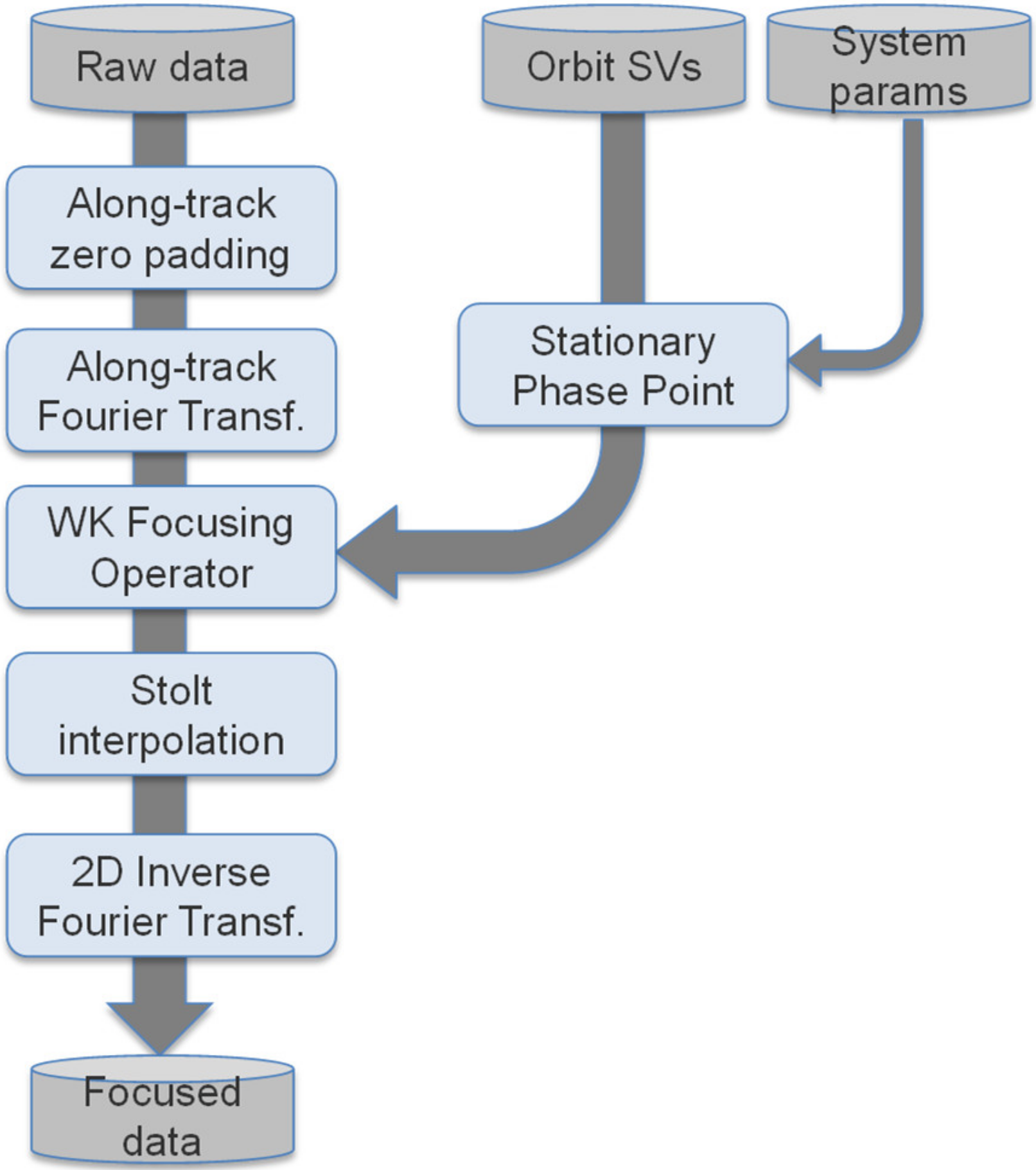
4. Implementation of WK F/F Algorithm

An overview of the main steps of the F/F algorithm is presented in Figure 3 and discussed below:
  • Along-track zero-padding of the raw data in the along-track direction. This processing step is needed since the along-track Fourier transform requires the time axis to be continuous and regularly spaced. In the case of closed-burst acquisition or when data acquisition is not continuous, raw data are zero-padded to fill the gaps in the non-continuous time axis. In case the ratio between the pulse and the burst repetition frequency is not an integer, an interpolation of the raw data must be implemented on a uniformly sampled time axis of reference. It has to be remarked that the impulse response function of the interpolator filter may condition the final shape of the focused IRF and this should be accounted for in an operational processor. We verified that a piecewise cubic Hermite interpolating polynomial (PCHIP) or a spline is sufficient for the treated case.
  • The dataset is Fourier-transformed in the along-track direction, range by range. The theoretical reference is in Equation (3) but, in practice, the FFT algorithm is used.
  • SPP solution. This block finds the stationary point x 0 by solving: d [ Φ t o t ( x ) ] d x | x 0 = 0 . The stationary point is a function of both   k x and t , that is, it can be evaluated, in principle, for every value of the Doppler frequency and of the fast time t . However, finding the roots of a fourth-order polynomial in all the along- and across-track positions may be computationally expensive (For a data block as long as an antenna footprint on ground, the minimum orbit length necessary to process is two times this length. This would correspond, using parameters in Table 1, to about 10 millions of samples for each block). A coarser grid is used in practice, obtaining the WK-focusing operator in the remaining positions by interpolation.
  • Along-track compression, which consists in the multiplication of the transformed dataset by the focusing operator sample-by-sample, according to Equations (10) and (11).
  • Stolt interpolation. After the compensation, the spectral support data is in the ( k x , t ) coordinates, while data must be represented in the ( k x , k r ) coordinates (i.e., the transformed plane corresponding to the image space). The non-separable mapping between the two domains is commonly implemented by the Stolt interpolation. For a monochromatic wave, the relation between the wavelength and the wavenumber in along- and across-track directions is
    ω = c 2 k x 2 + k r 2
    where ω = 2 π c λ ,   k x = 2 π λ sin ϑ , k r = 2 π λ cos ϑ , and ϑ is the incidence angle. The Stolt interpolation, in the time domain, still corresponds to a non-separable mapping from the data space   ( η , t ) to the image space ( x , τ r ) . In the altimeter case, Equation (14) can be rearranged considering ω = 2 π α t , k x = 2 π v e q f a , and k r = 2 π c 2 τ r . The Stolt mapping is a rather heavy interpolation of the equally spaced ω domain into a nonregularly spaced ω axis, as a function the regular sampling of the across-track wavenumber axis k r and of k x . One of the proposed simplifications, according to the acquisition geometry, consists in using a first order approximation ( k x -dependent) of the square root:   ω i 1 k x 2 ( 2 c ω 0 ) · k r ( 1 k x 2 ( 2 c ω 0 ) ) ω 0 with k r equally spaced on the across-track wavenumber axis.
  • Double inverse Fourier Transform completes the focusing, according to Equations (11) and (12). This is performed by applying the IFFT algorithm for the along-track and the FFT for the across-track directions.
  • Across-track compensation, which is aimed at compensating the across-track antenna G c r ( τ r ) , according to Equation (2), and the impact on the signal amplitude of the reduced Doppler history as a function of the range (see Appendix B for details).
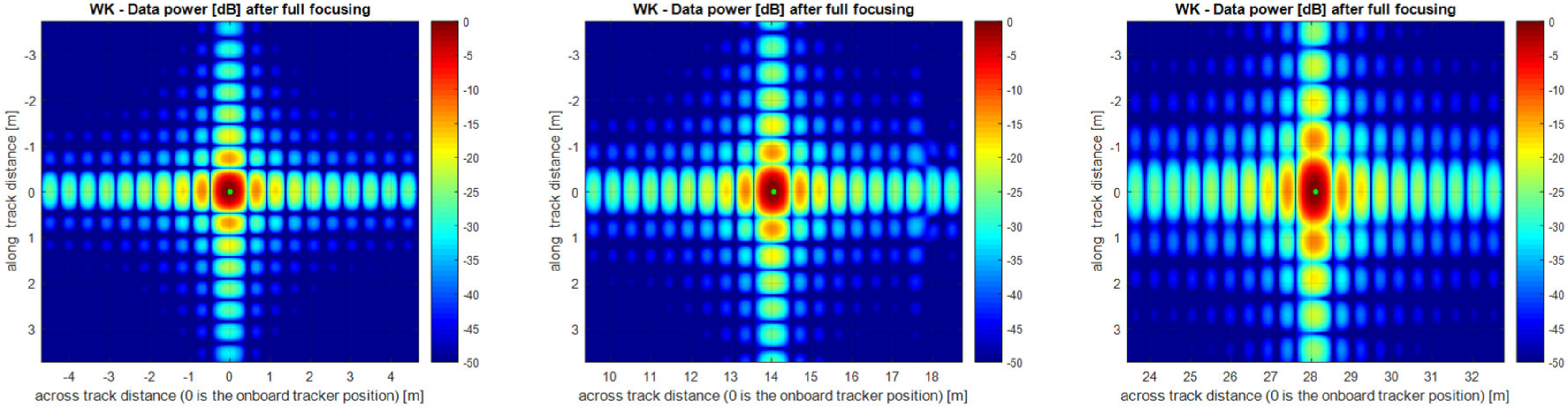
Further considerations for an accurate implementation should include a discussion on the following aspects: the density of the grid on the data block for the search of the stationary point; the kind and length of the interpolator to be used for along-track zero padding for the stationary point evaluation and Stolt interpolation. Moreover, it is important to consider the position of the tracker within the across-track window and the level of accuracy required in the evaluation of the stationary point in the case of a non-circular orbit. However, we deemed these aspects too practical and thus out of the scope of this paper.

5. Results

Experimental results were obtained by means of point target simulations and for CryoSat in-orbit data.

5.1. Simulation Results

The simulation approach for the point target is based on the unfocused IRF in Equation (2) and assumptions in Section 2.1. Additionally, it is remarked that the results presented in this section were obtained for a closed-burst configuration defined by the parameters in Table 1 and for a fixed tracking distance for the whole simulation, avoiding the handling of tracker changes within the scene. The on-board tracking point (i.e., the estimated average sensor-Earth distance used as the reference for the echo delay) was fixed at ¼ of the range window if not otherwise stated.
In Figure 4 and Figure 5, the 2D-focused IRF and the along- and across-track cuts are reported. The targets far from the tracker position show a decreased along-track resolution because of the reduced length of the Doppler history captured by the window extent (see Appendix B for details).
The quality of the focused IRF was assessed by comparison of WK with the back projection (BP) algorithm described in Reference [14]. In Figure 6, the 2D-focused IRF, and along- and across-track cuts are compared at the tracker position. As can be seen, the two algorithms produce very similar results. The comparison for the other positions are not reported here but the results are still very good. Moreover, the simulation was repeated for a target at the range window center but using a tracker in a different position (at ½ of the range window extent) and the results were again very similar.
The focused IRF obtained with the two different algorithms was compared using the IRF performance parameters, such as mainlobe −3 dB width, peak-to-side lobe ratio (PSLR), and position of the maximum with respect to the nominal target position (i.e., target’s mislocation). The comparison is shown in Table 2, where, additionally, the theoretically expected IRF quality parameters are also indicated as reference.
Along- and across-track resolutions for both WK and BP seem better than that theoretically predicted. This occurs for few centimeters or less and is basically due to the fact that, in practice, the shape of the IRF is not exactly a sinc. A small deformation due to alias contribution or grating lobes prevent the generation of a perfect IRF. For this reason, the energy is distributed differently in the main and secondary lobes compared to a sinc function. For the same reason, the better resolution in along-track for BP w.r.t. WK is paid by more energy in sidelobe: −13.27 dB (BP) compared to −14.05 dB (WK) for along-track PSLR. Finally, since the along- and across-track misalignments are a function of the measurement precision and since the IRF function shape is achieved by means of oversampling, we reported the measurement precision in Table 2.
Residual amplitude and phase distortion is still present using WK focusing. Such distortion, along- and across-track-dependent, is due to several reasons, such as the approximate estimation of the stationary point, the effect of the interpolators used for along-track zero padding and Stolt interpolation, and aliasing due to the not perfect filtering of the antenna mainlobe. To evaluate the amount of distortion in the two directions, a regularly spaced grid of point targets was deployed within the data block. A total of 121 targets, arranged in a grid of 11 × 11, were placed at regular spacing of 6 samples in across-track (about 2.81 m) and 2400 lines in along-track (about 894 m), so to uniformly cover a large part of the data block, which is as large as an antenna footprint on ground (around 13 km). The target amplitude and phase were set in the simulation to 1 and 0, respectively. After WK focusing, the amplitude and phase were compared with the expected values, resulting in a worst-case amplitude distortion equal to 0.19 dB. Repeating the same experiment for BP, the distortion is smaller than 0.05 dB. The phase distortion, instead, results in a linear phase across-track, with a slope basically invariant in the along-track direction. WK focusing implementation can be refined to mitigate the residual distortions and the authors are still working in this direction.

5.2. Computational Evaluation

The estimation of the computational effort through the number of complex multiplications per output sample was performed on a data-block basis. One-time processings that does not involve the data block have not been included, since it is supposed that in ideal conditions such processings are done one time while data are processed on a block-by-block basis many times.
The WK algorithm is by far faster and computationally less intensive than the BP algorithm. Table 3 shows the comparison of the number of complex multiplications per output sample and processing time estimated to process an acquisition of about 4.15 s (i.e., 351 bursts), using parameters in Table 1 in the BP and WK algorithm cases. The last two columns report, instead, the theoretical (and simplified) computation of the number of complex multiplications per output sample. The number in the last column, in principle, should be an estimate of the number in the first one.
For the BP algorithm, the number of complex multiplications per output sample is
N B P , c o s t = N i l l · N r + N i l l · N r · N r l o g 2 N r + N i l l · N r + 2 N i l l · N r N r = N i l l · ( 4 + l o g 2 N r )
In the numerator, the first term accounts for the multiplication of the range migration correction term; the second term accounts for the range compression (an FFT); the third term is the multiplication for the compensation of the residual video phase; finally, the fourth term is the antenna gain and the RRP compensation (for details on the BP processing steps, see Reference [13]). The output so achieved is valid for all the samples in the same along-track position; thus, the number of complex multiplications per output sample is achieved after division by N r . For the current parameters, this number is about 123,000.
In the case of the WK algorithm, the theoretical cost for a block of data is (perhaps slightly underestimated)
N W K , c o s t = 4 ( s N b l ) N r + N r · s N b l · l o g 2 ( s N b l ) + N r · s N b l · [ ( 8 3 n 3 + n 2 + 5 ) 1 D 1 D 2 + 4 · 4 ] + N r · s N b l + 4 N r · s N b l + N r · s N b l · [ l o g 2 ( s N b l ) + l o g 2 N r ] + N r · s N b l + 4 N r · s N b l / 2
where:
-
the first term is due to zero-padding (interpolation kernel length is 4 for a piecewise cubic Hermitian interpolator);
-
the second term is the cost of the along-track Fourier transform, being s the increasing factor due to zero-padding, which is about s = P R I / B R I (for the current parameter, s is about 3.5);
-
the third term is due to the SPP computation and includes the solution of the fourth-order polynomial. To solve the polynomial equation, Singular Value Decomposition is used in practical algorithms and its cost in term of multiplications is about 8 3 n 3 + n 2 (with n being the polynomial order). This is repeated for each sample of the coarser grid (subsampled at D1 in along-track and D2 in across-track). The further 5 multiplications are due to the generation of the polynomial coefficients and the final 4 to make the interpolation on the full grid of   N r · s N b l samples.
-
The fourth term is due to the focalization and along-track antenna compensation
-
The fifth term is due to the Stolt interpolation
-
The sixth term is due to the 2D inverse Fourier transform
-
The seventh term is due to the across-term antenna compensation
-
The eighth term is due to the interpolation on the output samples (that are approximately half the size in along-track).
Both the algorithms were run on a Intel® Core i7-4790 @3.60 GHz equipped with 16 GB RAM and using Matlab®. The comparison of the first and second rows shows the higher efficiency of the WK algorithm in terms of complex multiplication (almost 1000 times) and computational time (over 500 times). More efficient implementation environment (compiled C++ or Java) or dedicated machine (a Graphic Processing Unit, GPU) could allow the further reduction of processing time, arriving to a near real-time implementation (i.e., about 4 s of processing for 4 s of acquisition).

5.3. WK Algorithm on CryoSat in-Orbit Data

In this section, a demonstration of the WK algorithm is given by processing an in-orbit CryoSat acquisition in the SAR mode over the Svalbard transponder. Since the transponder acts like a point target with high power with respect to the noise and surrounding clutter, it allows to verify the effectiveness of the focusing algorithm with in-orbit data by inspection of the characteristics of the focused IRF. To perform this analysis, we used ESA CryoSat Full Bit Rate (FBR) Baseline-C data and we applied calibration corrections according to Reference [18]. The following results were obtained processing the pass over the Svalbard transponder that was acquired by CryoSat on 21 August 21 2012 around 22:42 UTC time.
The WK algorithm implementation described in Section 4 was used to process the CryoSat FBR data. For passes over a transponder, CryoSat/SIRAL is commanded to keep a constant value for the on-board tracker, so that additional processing steps to align the echoes are not needed. Being not applicable the circular orbit approximation in the case of in-orbit data, a polynomial fitting of the fourth order was adopted to the piece of orbit covering the transponder acquisition. Finally, the processed bandwidth was limited to 25% of the total Doppler bandwidth, so that an along-track resolution lower than the theoretical one was expected. Limiting the processed bandwidth was needed since a residual along-track phase contribution was found when processing in-orbit CryoSat acquisitions, regardless of the focusing algorithm (BP or WK). The cause of this residual phase was identified and fixed in our in-house implementation of the BP algorithm, while it still has not been used in the prototype implementation of the WK algorithm.
Figure 7 shows the focused IRF that was obtained by focusing the CryoSat FBR data with the WK algorithm. When inspecting Figure 7, it can be noticed that the 2D IRF is sinc-like in both the directions as expected with PSLR closer to the theoretical expected values. The across-track resolution at −3 dB is approximately 0.424 m and the along-track resolution at −3 dB is approximately 2.24 m. It has to be remarked that, even by reducing the processed bandwidth to 25% of the Doppler bandwidth, an along-track resolution in the order of a few meters is achieved, in comparison with the along-track resolution two orders of magnitude higher that can be obtained with Delay/Doppler processing.
Figure 8 shows the 2D focused IRF in a wider interval of the along-track distance. Since CryoSat operates with a closed-burst timeline, the obtained 2D IRF is characterized by grating lobes in along-track spaced at approximately 90.5 m, as discussed in Section 3, and partially focused farther away from the point target location, as discussed in Appendix A.
We finally verified that the focused IRF is not a function of the target along the track position when the circular orbit assumption does not hold, as for in-obit CryoSat data. By selecting different blocks of bursts from FBR to be processed, the transponder was focused at different distances from the center of the scene used as reference point to determine the sensor-target distance. It is worth noting that the selected blocks cover 2 s of acquisition, and the transponder acquisition here considered is characterized by an altitude rate of about −12.5 m/s. By comparing the 2D IRF in Figure 7, which was obtained placing the transponder at the center of the scene, and the 2D IRF in Figure 9, which was obtained placing the transponder 6000 m away from the center of the scene, it can be noticed that the 2D IRF is well focused also when the target is at the edge of the block. Figure 9 also shows the comparison of the along-track cuts obtained placing the transponder at different distances from the center of the scene. There, it can be observed that the shape of the IRF does not sensibly depend on the along-track position of the target. When placing the transponder at 6000 m from the center of the scene, the along-track resolution at −3 dB is approximately 2.25 m.
The WK algorithm implementation was used to process a CryoSat SAR acquisition over sea ice. The FBR product CS_OFFL_SIR1SAR_FR_20170112T234631_20170112T235640_C001.DBL [22] was processed; in Figure 10, the power waveforms obtained with FFSAR WK are visually compared with the power waveforms from the corresponding CryoSat Baseline-C L1b product, which are at 20 Hz posting rate from a Delay/Doppler processor. Figure 10 shows the radargram obtained with FFSAR WK processing both at PRF rate and at 20 Hz, after time domain incoherent multilooking. The color scale of the different radargrams has been adjusted to show that similar structures are present in all the radargrams.

6. Discussion and Conclusions

This paper presents an efficient focusing algorithm for high PRF radar altimeters that is performed in a two-dimensional wavenumber domain. We showed that by reformulating the exact transfer function, it is possible to obtain an exact focusing as in the usual SAR case, gaining in terms of computational effort (i.e., number of complex multiplications per output sample) and computational time with respect to the traditional back projection algorithm. Using a simulation, we verified that echoes from both closed-burst and open-burst acquisition modes can be focused at full resolution using the proposed algorithm. The effectiveness of the proposed algorithm has been demonstrated using simulated data in order to assess performance in terms of quality of the focused IRF as well as computational burden. Additionally, the applicability of the proposed fully focused algorithm to in-orbit acquisitions from a high PRF radar altimeter instrument has been proved by successfully focusing CryoSat FBR data over a transponder.
However, implementing a complete fully-focused SAR processing chain, able to generate Level-1 products, is a challenging perspective for both existing and future altimetry missions. This would allow increasing the accuracy of the estimation of target positions, which is a particularly relevant requirement to detect surface transitions in sea-ice or inland water scenarios. For this reason, unsolved or open issues such as an efficient mitigation scheme for the grating lobes as well as the reformulation of the algorithm for altimeter instruments based on on-board matching filter on receive will be addressed and investigated shortly.

Author Contributions

P.G. solved the theoretical problem, wrote the paper, and conceived the simulations. M.S. wrote the paper, contributed to many parts of the algorithm implementation, and took care of the in-orbit data focusing. D.G. coordinated the study, corrected the paper, and wrote the final section.

Funding

This research received no external funding

Acknowledgments

The authors wish to acknowledge the European Space Agency for its valuable support and funding for this study under Contract 4000116663/16/NL/IA.

Conflicts of Interest

The authors declare no conflict of interest.

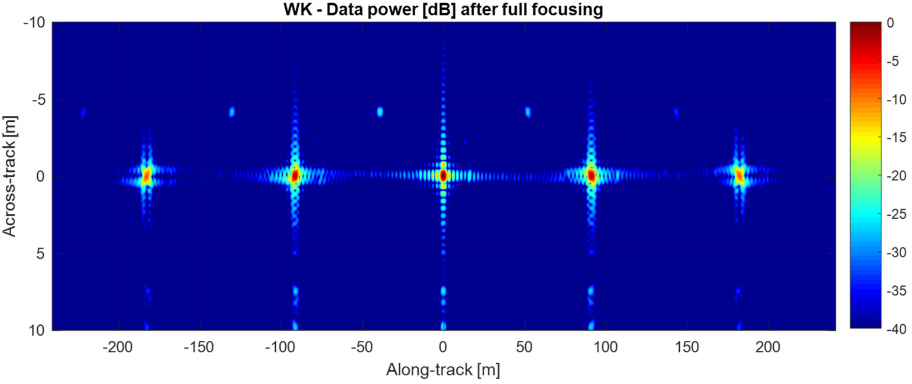
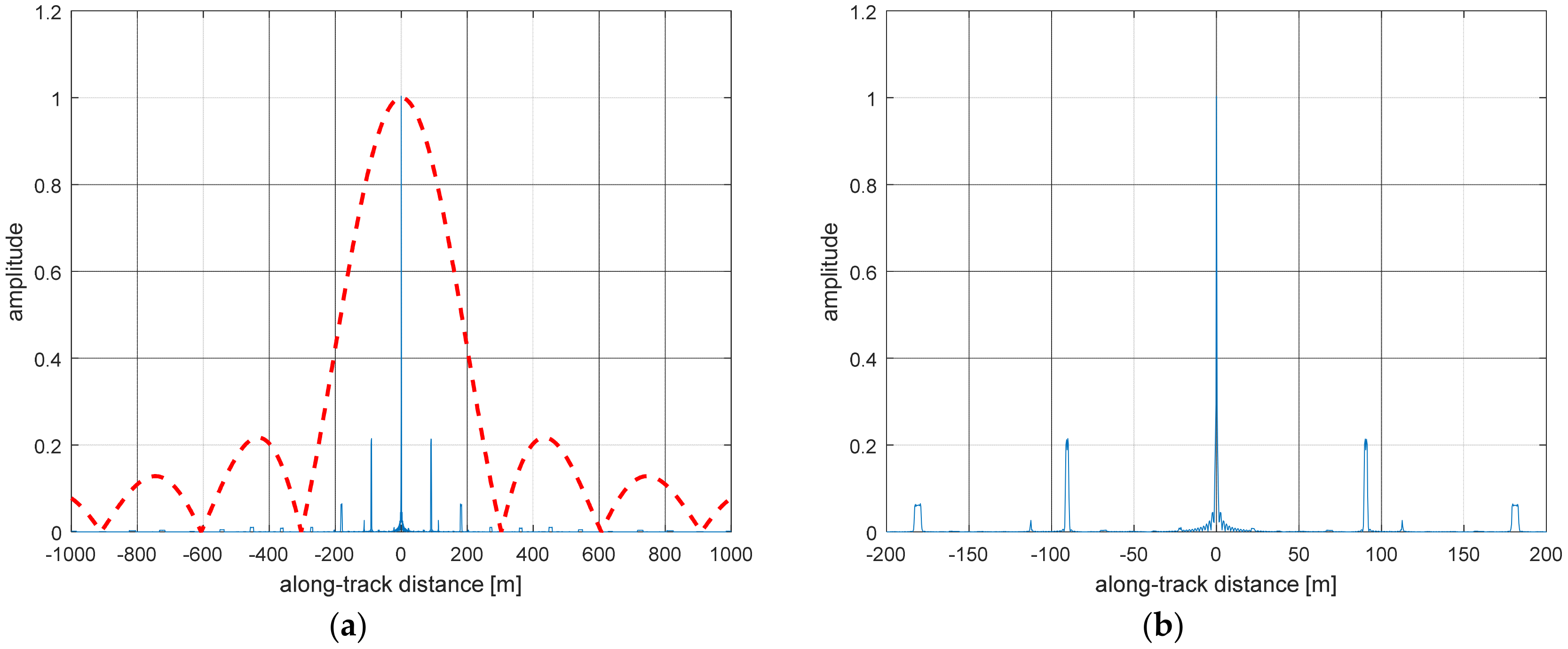
Appendix A. Grating Lobes

Taking again the expression of the focused IRF (Equation (11)),
h f o c ( η , τ r ; R t k r ) = W B W p · s i n c ( B c h τ r ) · s i n c ( W B η ) · n s i n c [ B d o p ( η η 0 n W p ) ]
we already recognized the presence of repeating peaks at distance Δ y g r = v α T 1 W p 90.5   m . Since the focusing operator is exact in the stationary phase point x 0 only, and being x 0 a function of the along- and across-coordinates η and   t , the grating lobes are expected to be not exactly focused in across-track, as they do not correspond to the true target position. In Figure A1, the along-track cut of a focused point target is imaged using the parameters in Table 1. As can be seen (Figure A1b), the grating lobes are spaced as expected but their width (especially for far lobes) tends to increase due to blurring. As a consequence, their height is not the nominal one, given by the D/D envelope (dotted red line in Figure A1a, because of the spread of energy in across-track.
Clearly, the grating lobes represent an impairment in the F/F IRF and any technique that is aimed at removing them (e.g., deconvolution algorithm) cannot use the exact formulation in Equation (13) to compensate the grating lobes around a given target position, due to defocusing.
Figure A1. Along-track cut of a focused IRF target put in the tracker position. Parameters in Table 1 have been used in the simulation. (a) The interval [−1000, 1000] m with superimposed D/D envelope s i n c ( W B η ) (red-dotted line); (b) detail around the main lobe.
Remotesensing 10 01943 g0a1

Appendix B. Doppler History Length Variability

Each target is seen by a limited number of sensor positions because of the limited extent of the receiving range window. This fact is illustrated by showing the Doppler history (after range compression) of three targets put in different across-track positions before (Figure A2a) and after (Figure A2b) range migration correction. As it can be seen, the length of the Doppler history decreases as the range position of the target increases, since it is cut on board by the limited instrument receiving window.
Figure A2. Doppler history of three targets in different across-track positions (Table 1 parameters used). (a) After range compression; (b) after range compression and range migration compensation.
Remotesensing 10 01943 g0a2
This fact has two consequences: (i) the resolution in along-track worsens for far across-track positions, since less return means also less Doppler band acquired; (ii) the targets’ amplitude at far range is reduced because of the lower number of summing contributions. While the second consequence should be corrected to produce a radiometrically calibrated product, the first is unavoidable and produces the different along-track resolutions for such targets, as already shown in Figure 4 and Figure 5.

References

  1. Rey, L.; de Chateau-Thierry, P.; Phalippou, L.; Mavrocordatos, C.; Francis, R. SIRAL: The radar altimeter for CryoSat mission, under development. In Proceedings of the IEEE International Geoscience and Remote Sensing Symposium, Toronto, ON, Canada, 24–28 June 2002; Volume 3, pp. 1768–1770. [Google Scholar]
  2. Raney, R.K. The delay/Doppler radar altimeter. IEEE Trans. Geosci. Remote. Sens. 1998, 36, 1578–1588. [Google Scholar] [CrossRef]
  3. Wingham, D.J.; Phalippou, L.; Mavrocordatos, C.; Wallis, D. The mean echo and echo cross-product from a beam forming, interferometric altimeter and their application to elevation measurement. IEEE Trans. Geosci. Remote. Sens. 2004, 42, 2305–2323. [Google Scholar] [CrossRef]
  4. Parrinello, T.; Shepherd, A.; Bouffard, J.; Badessi, S.; Casal, T.; Davidson, M.; Fornari, M.; Maestroni, E.; Scagliola, M. CryoSat: ESA’s ice mission—Eight years in space. Adv. Space Res. 2018, 62, 1177–1638. [Google Scholar] [CrossRef]
  5. Donlon, C.; Berruti, B.; Buongiorno, A.; Ferreira, M.-H.; Femenias, P.; Frerick, J.; Goryl, P.; Klein, U.; Laur, H.; Mavrocordatos, C.; et al. The Global Monitoring for Environment and Security (GMES) Sentinel-3 Mission. Remote. Sens. Environ. 2012. [Google Scholar] [CrossRef]
  6. Scharroo, R.; Bonekamp, H.; Ponsard, C.; Parisot, F.; von Engeln, A.; Tahtadjiev, M.; de Vriendt, K.; Montagner, F. Jason continuity of services: Continuing the Jason altimeter data records as Copernicus Sentinel-6. Ocean Sci. 2016, 12, 471–479. [Google Scholar] [CrossRef]
  7. Laxon, S.W.; Giles, K.A.; Ridout, A.L.; Wingham, D.J.; Willatt, R.; Cullen, R.; Kwok, R.; Schweiger, A.; Zhang, J.; Haas, C.; et al. CryoSat-2 estimates of Arctic sea ice thickness and volume. Geophys. Res. Lett. 2013, 40, 732–737. [Google Scholar] [CrossRef] [Green Version]
  8. Gourmelen, N.; Escorihuela, M.J.; Shepherd, A.; Foresta, L.; Muir, A.; Garcia-Mondejar, A.; Roca, M.; Baker, S.G.; Drinkwater, M.R. CryoSat-2 swath interferometric altimetry for mapping ice elevation and elevation change. Adv. Space Res. 2017. [Google Scholar] [CrossRef]
  9. Boy, F.; Desjonquères, J.D.; Picot, N.; Moreau, T.; Raynal, M. CryoSat-2 SAR-Mode Over Oceans: Processing Methods, Global Assessment, and Benefits. IEEE Trans. Geosci. Remote. Sens. 2017, 55, 148–158. [Google Scholar] [CrossRef]
  10. Bonnefond, P.; Laurain, O.; Exertier, P.; Boy, F.; Guinle, T.; Picot, N.; Labroue, S.; Raynal, M.; Donlon, C.; Féménias, P.; et al. Calibrating the SAR SSH of Sentinel-3A and CryoSat-2 over the Corsica Facilities. Remote. Sens. 2018, 10, 92. [Google Scholar] [CrossRef]
  11. Dinardo, S.; Fenoglio-Marc, L.; Buchhaupt, C.; Becker, M.; Scharroo, R.; Fernandes, M.J.; Benveniste, J. Coastal SAR and PLRM altimetry in German Bight and West Baltic Sea. Adv. Space Res. 2018, 62, 1371–1404. [Google Scholar] [CrossRef]
  12. Boergens, E.; Nielsen, K.; Andersen, O.B.; Dettmering, D.; Seitz, F. River Levels Derived with CryoSat-2 SAR Data Classification—A Case Study in the Mekong River Basin. Remote. Sens. 2017, 9, 1238. [Google Scholar] [CrossRef]
  13. Raney, R.K. CryoSat SAR-mode looks revisited. IEEE Geosci. Remote. Sens. Lett. 2012, 9, 393–397. [Google Scholar] [CrossRef]
  14. Egido, A.; Smith, W.H.F. Fully Focused SAR Altimetry: Theory and Applications. IEEE Trans. Geosci. Remote. Sens. 2017, 55, 392–406. [Google Scholar] [CrossRef] [Green Version]
  15. Holzner, J.; Bamler, R. Burst-Mode and ScanSAR Interferometry. IEEE Trans. Aerosp. Electron. Syst. 2002, 40, 1917–1934. [Google Scholar] [CrossRef]
  16. Bamler, R. A Systematic Comparison of SAR Focusing Algorithms. In Proceedings of the IGARSS ’91 Remote Sensing: Global Monitoring for Earth Management: 1991 International Geoscience and Remote Sensing Symposium, Espoo, Finland, 3–6 June 1991; pp. 1005–1009. [Google Scholar]
  17. Cafforio, C.; Prati, C.; Rocca, F. SAR data focusing using seismic migration techniques. IEEE Trans. Aerosp. Electron. Syst. 1991, 27, 194–207. [Google Scholar] [CrossRef]
  18. Scannapieco, F.; Renga, A.; Moccia, A. Indoor Operations by FMCW Millimeter Wave SAR Onboard Small UAS: A Simulation Approach. J. Sens. 2016. [Google Scholar] [CrossRef]
  19. Curlander, J.C.; McDonough, R.N. Synthetic Aperture Radar—System and Signal Processing; Wiley: Hoboken, NJ, USA, 1991; ISBN 978-0-471-85770-9. [Google Scholar]
  20. Carrara, W.G.; Goodman, R.S.; Majewski, R.M. Spotlight Synthetic Aperture Radar: Signal Processing Algorithms; Artech House: Norwood, MA, USA, 1995; ISBN-13: 978-0890067284. [Google Scholar]
  21. Paupolis, A. Systems and Transforms with Applications in Optics; R. Krieger Publishing Company: Malabar, FL, USA, 1968; ISBN-10 0070484570. [Google Scholar]
  22. C2-TN-ARS-GS-5179, CryoSat Characterization for FBR Users Corrections. June 2016. Available online: https://wiki.services.eoportal.org/tiki-download_wiki_attachment.php?attId=4233&page=CryoSat% 20Technical%20Notes&download=y (accessed on 28 February 2010).
Figure 1. Acquisition geometry of a high pulse repetition frequency (PRF) altimeter in closed-burst configuration. Notation according to Table 1.
Remotesensing 10 01943 g001
Figure 2. Doppler spectrum of a simulated point target. (a) Non-ambiguous Doppler spectrum (the antenna shape is visible); (b) detail around 0 Hz: strips of band W B = 22.3 Hz and distant W p ≈ 74.8 Hz can be recognized.
Remotesensing 10 01943 g002
Figure 3. Algorithm scheme.
Remotesensing 10 01943 g003
Figure 4. 2D focused impulse response function (IRF) of targets at different across-track positions. From left to right: target at tracker position, target at 30 and 60 samples across-track far. Closed-burst simulation using parameters in Table 1.
Remotesensing 10 01943 g004
Figure 5. Along-track (left) and across-track (right) cuts of the focused targets in Figure 4. Across-track cuts are perfectly superimposed.
Remotesensing 10 01943 g005
Figure 6. Upper row: 2D-focused IRF of target tracker position. Left: WK algorithm; right: BP algorithm. Lower row: along- (left) and across-track (right) cuts for the focused IRF of upper row. Closed-burst simulation using parameters in Table 1.
Remotesensing 10 01943 g006
Figure 7. Focused IRF obtained by processing CryoSat FBR over transponder: 2D IRF (left), along-track cut (center), and across-track cut (right).
Remotesensing 10 01943 g007
Figure 8. 2D focused IRF obtained by processing CryoSat FBR over transponder in the along-track interval [−240, 240] m around the transponder location.
Remotesensing 10 01943 g008
Figure 9. Focused IRF obtained by placing the transponder far from the center of the scene: 2D IRF at 6000 m from the centre of the scene (left), along-track cuts at different distances from the center of the scene (right).
Remotesensing 10 01943 g009
Figure 10. Radagram for sea ice CryoSat acquisition: FFSAR WK at PRF rate (left), FFSAR WK subsampled at 20 Hz rate (center), and Delay/Doppler at 20 Hz (right). Elevation over the ellipsoid is on the y-axis.
Remotesensing 10 01943 g010
Table 1. Symbols used in the paper 1 and reference numbers adopted in simulations.
SymbolDescriptionUsed Values/UoM
τ Across-track times
t Time varying within the pulse duration: | t | T p / 2 s
η Along-track times
T p Pulse duration45 μs
f c Carrier frequency13.6 GHz
f r g Range sampling frequency320 MHz
α Chirp rate7.14 × 1012 Hz/s
PRFPulse repetition frequency18.2 kHz
BRFBurst repetition frequency85 Hz
β 3   d B Along-track antenna beam width (−3 dB)0.019 rad
{ N r , N a z } Number of samples in across-track and pulses in a burst{128, 64}
h 0 Average altitude730 km
R T Local Earth radius6371 km
R t k r Tracker distance R t k r h 0
v r Radial velocitym/s
Δ Doppler coefficient Δ = 2 v r ( η ) / c
f D Doppler centroid Δ · f c [Hz]
1 Values used throughout the paper are very close to those of the CryoSat system and geometry.
Table 2. Comparison of focused IRF quality parameters for target positioned in 0 and 40 samples far from tracker positions and at 0, 1500 along-track lines from scene center. Table 1 parameters have been used.
Target (rg, az)MethodAlong-Track ResolutionAcross-Track ResolutionPSLR 2nd [dB] Along/AcrossMisalingment Along-TrackMisalignment Across-Track
0, anyTheoret.0.421 m0.415 m −13.26
40, anyTheoret.0.554 m0.415 m
0, 0WK0.419 m0.410 m−14.05/−13.19<10−3 m<10−3 m
40, 0WK0.559 m0.410 m−13.26/−13.12<10−3 m<10−3 m
0, 1500WK0.419 m0.410 m−14.04/−13.19<10−3 m<10−3 m
0, 0BP0.407 m0.410 m−13.27/−13.17<10−3 m<10−3 m
40, 0BP0.536 m0.410 m−13.27/−13.18<10−3 m<10−3 m
0, 1500BP0.407 m0.410 m−13.27/−13.17<10−3 m<10−3 m
Table 3. Computational effort comparison of back projection (BP) and Omega-Kappa (WK) algorithm using parameters in Table 1.
MethodCost per Sample [cplx mult]Processing Time [s]Theoretical Cost per Output SampleApproximate Value Using Cryosat Parameters
BP134,5648978Equation (15)123,200
WK11416.8Equation (16)135

