2. Materials and Methods
2.1. Study Area
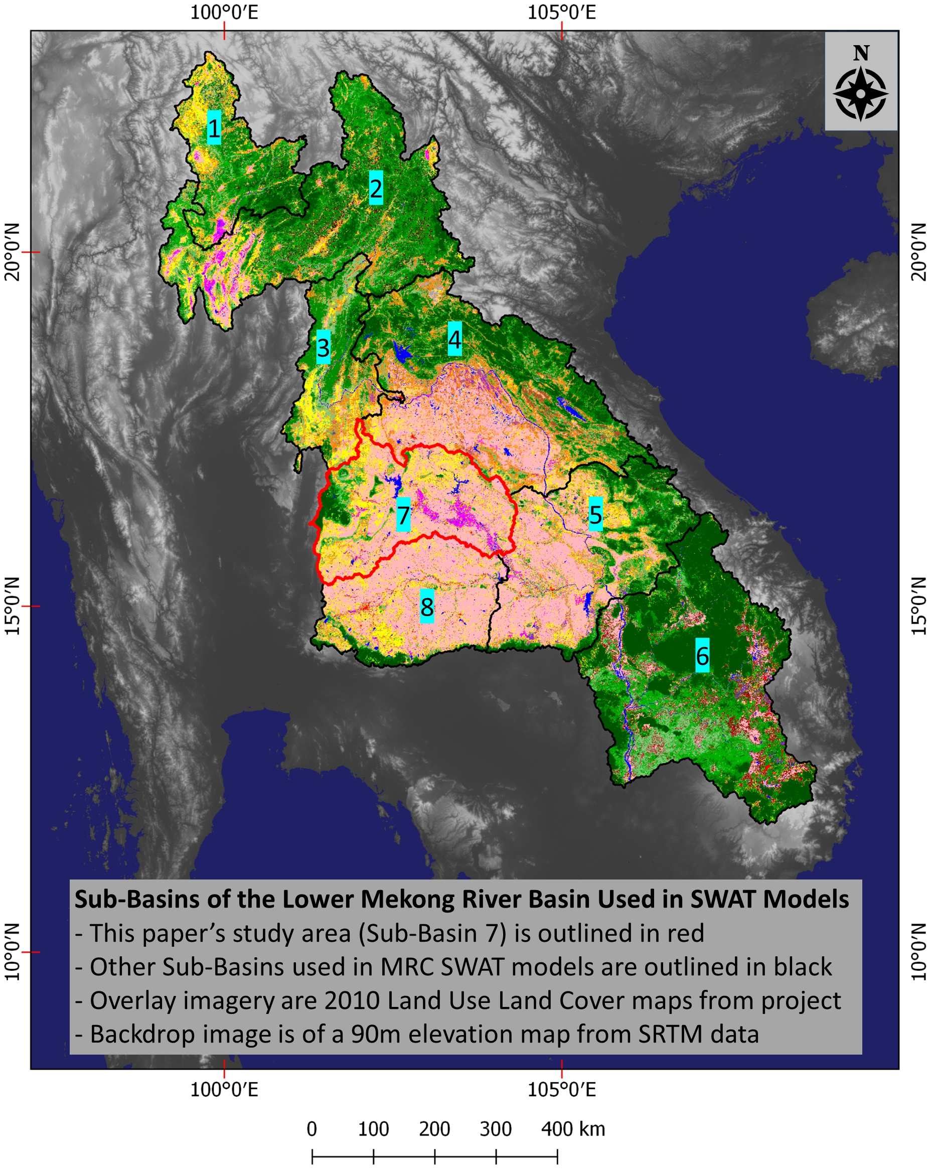
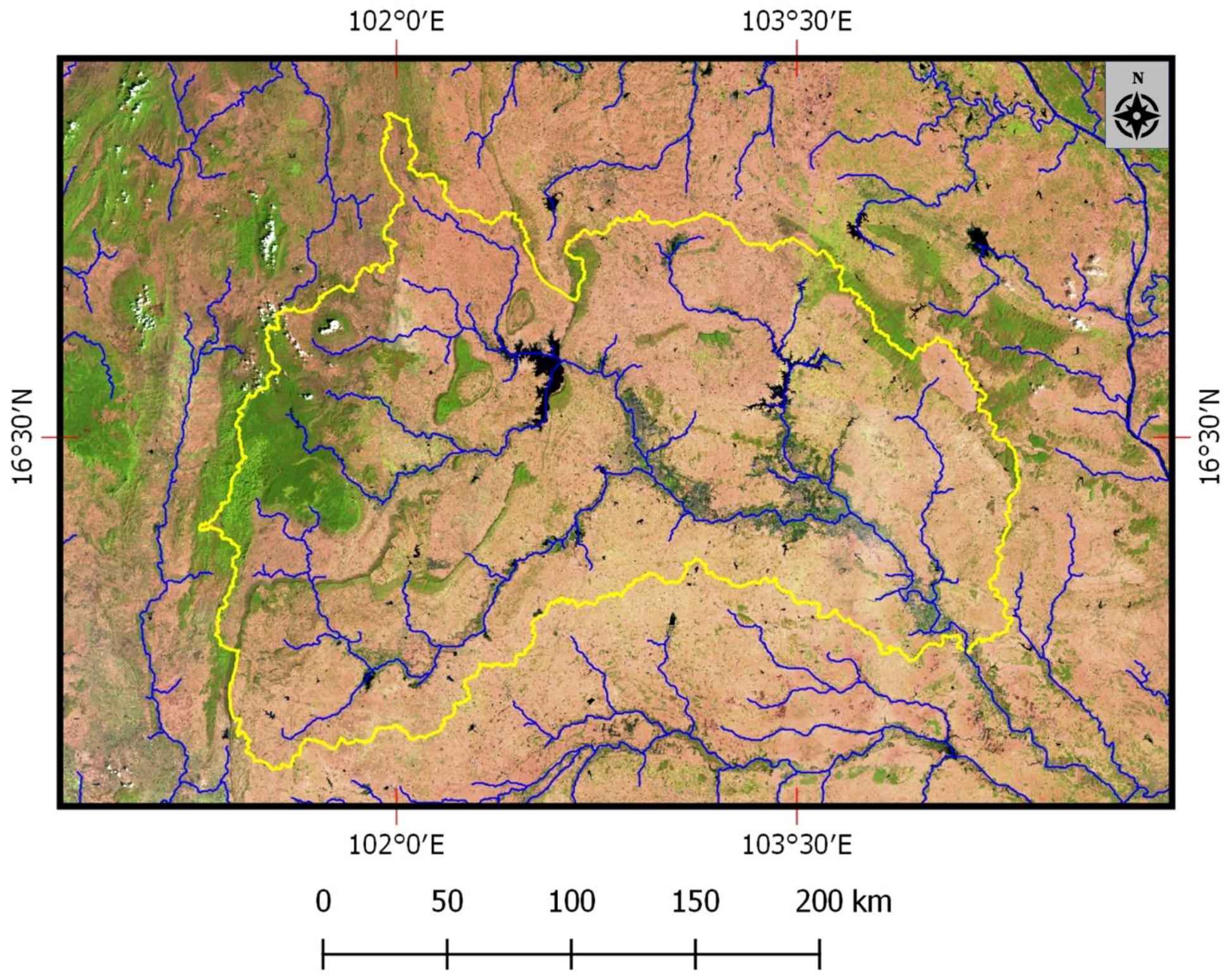
The study area is in the sub-basin (SB) 7 of the Lower Mekong Basin (LMB) (
Figure 1). The LMB includes areas in Cambodia, Laos, Myanmar, Thailand, and Vietnam. SB 7 is one out of 8 SBs that the MRC uses with the SWAT model to aid water and disaster management in the region [
1]. The study area includes in the central portion of the Khorat Plateau of Thailand and varies in elevation from 90 to 1326 m, based on NASA SRTM 30-m Digital Elevation Model (DEM) data [
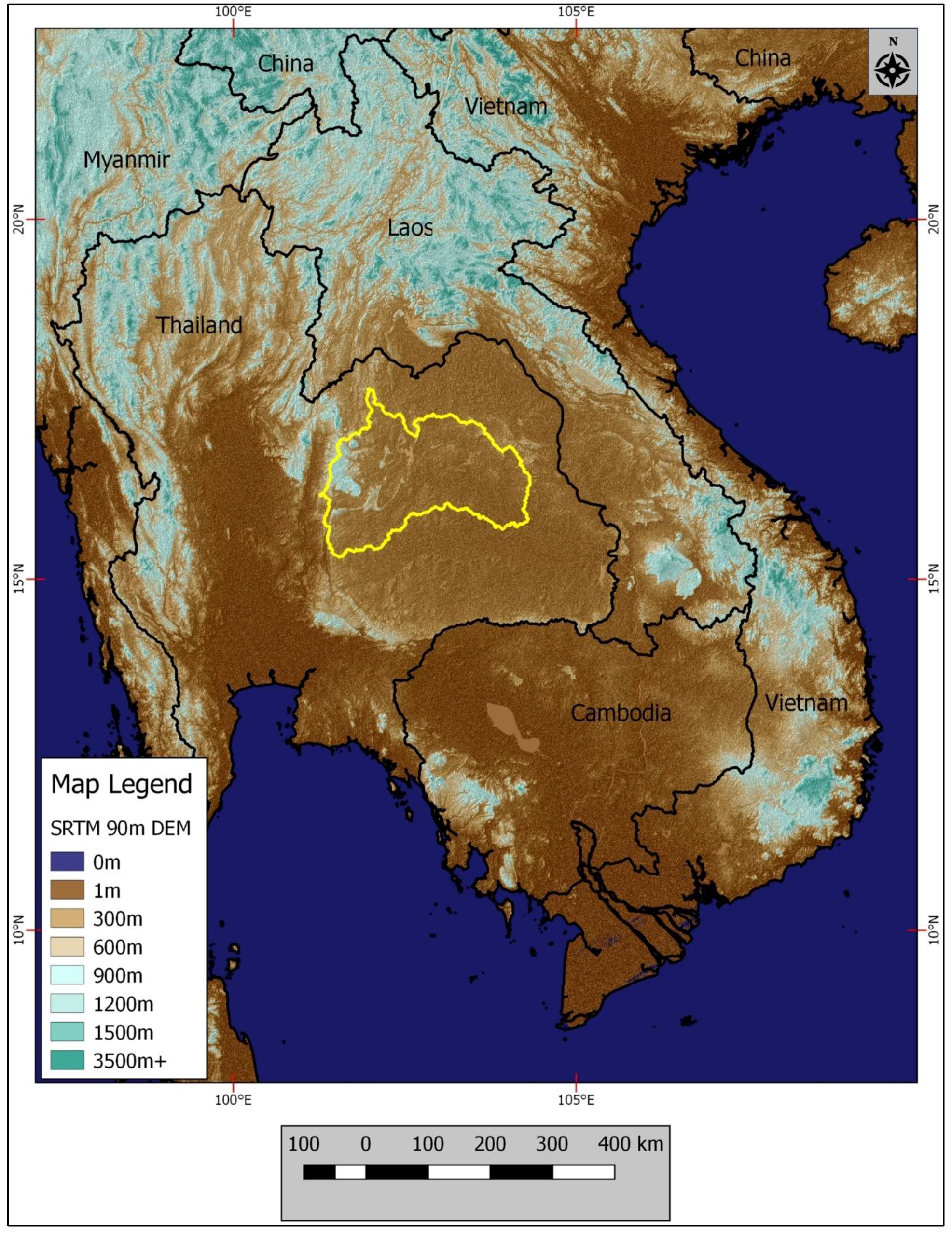
23]. As the main waterway in the SB, the Chu River runs into the Mun River which then flows into the Mekong River (
Figure 2).
The study area contains several LULC classes (
Figure 3) including multiple natural forest and agricultural types of interest to MRC SWAT modelers and relevant to water resource management. For the most part, the study area is an agriculturally dominated landscape in which single season rainfed rice and other mixed annual crops are grown. Along more prominent waterways, irrigated double-cropped rice can commonly occur. Shifting cultivation “slash and burn” agriculture is rare, compared to more forest dominated SBs in the LMB, such as in Lao PDR. Within the study area, some industrial forest plantations (e.g., rubber) occur amongst the main agricultural areas. Deciduous and evergreen broadleaved forests occupy portions in the study area and are primarily limited to higher elevation areas that are mainly managed as national parks. Bamboo scrub/forest occurs in some forest dominated areas. Wetlands with nonagricultural vegetation in the study area are comparatively rare, due to most wetland sites being converted to and managed for rice agriculture. A detailed description of forest LULC types of the study area is provided by [
24].
The study area includes a dry season that typically occurs from October through April. A wet (i.e., monsoon) season takes place from May to October [
24]. LMB cloud frequency is typically much higher during the wet season [
10].
2.2. Data Acquisition
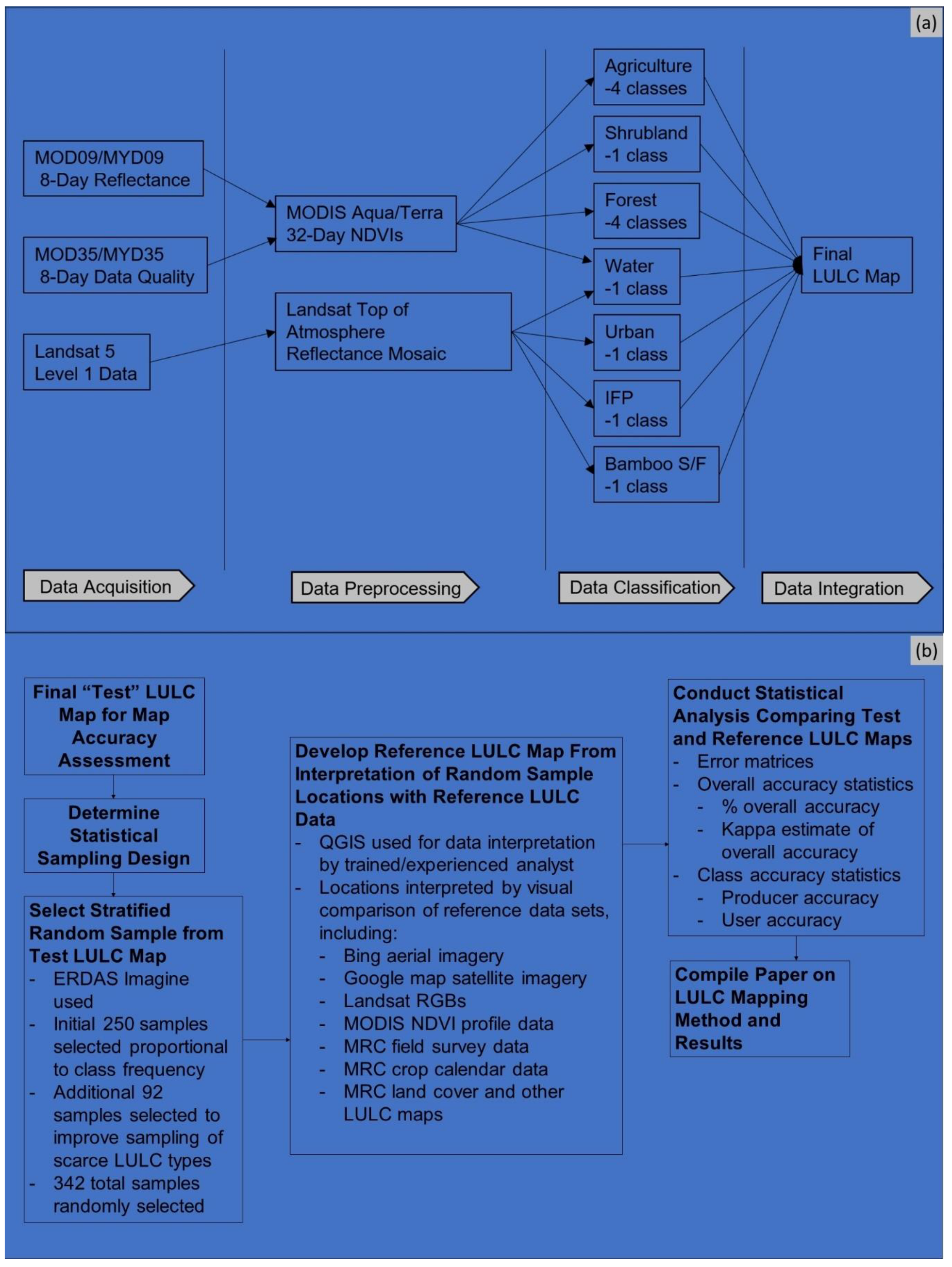
The basic work flow used in generating the LULC map for SB 7 is shown in
Figure 4. To initiate the mapping process, MODIS Collection 5 MOD09 and MYD09 8-day composited reflectance data at a qkm spatial resolution [
25,
26] were acquired for 2003 to 2011 from the LP DAAC, including data for tiles h27v06, h27v07, h28v07, and h28v08. Corresponding MODIS MOD35 and MYD35 cloud masking products [
27] were also acquired to assess and clean MODIS reflectance data for known data quality issues.
Level 1 Landsat Thematic Mapper data collected during the dry seasons (February) of 2009 to 2011 was downloaded from the USGS GloVis web site [
28], including data sets from 6 scenes with paths 127 (rows 48 and 49), 128 (rows 48 and 49), and 129 (rows 48 and 49). In addition, SRTM DEM data was acquired for the study area at 1 arc second (i.e., 30-m) resolution [
23]. Additional higher spatial resolution true color satellite and aerial imagery was accessed from Google and Bing web sites via the QGIS OpenLayers plugin [
29].
2.3. Data Preprocessing
Although MODIS Aqua and Terra sensors together collect two images per day for most of the human inhabited world, the data from these systems typically needs additional temporal processing to reduce cloud and cloud shadow impacts, especially for the cloud prone tropics. The LMB area is frequently cloudy, especially during the rainy season [
10,
24]. Even in temperate environments, effective production and use of MODIS-based time series of vegetation index products typically must include temporal processing to remove bad data and mitigate pixels for dates of data affected by atmospheric contamination. Also known as temporal processing, this type of data preprocessing is necessary as a precursor to LULC classification based on MODIS NDVI time series data sets.
The Time Series Product Tool (TSPT) was used in this project to perform temporal processing of the MODIS MOD09 and MYD09 8-day reflectance data. TSPT is a custom program developed with MATLAB computer programming software [
30,
31,
32]. TSPT has been used on numerous occasions to derive temporally process time series of vegetation index products. It enables such time series data sets to be processed in terms of bad data removal, data fusion, noise reduction, and data void interpolation [
14,
30,
31,
32].
TSPT data processing began with the ingest of MODIS Terra (MOD09) and Aqua (MYD09) 8-day data on an individual tile basis for a given year. Such 8-day products are less frequently cloud covered than daily reflectance data but still can include extensive areas (e.g., pixels) affected by atmospheric contamination, poor viewing geometry, and inherent data quality artifacts (e.g., from pixel and line drop outs). In this project, the goal of using TSPT was to temporally process both the 8-day MODIS Aqua and Terra reflectance data to derive annual 32-day merged MODIS Aqua/Terra NDVI time series that were much less visibly cloud-impacted than the original 8-day data sets and therefore more amenable to LULC classification. The processing of the annual time series for 2010 included 96 total MODIS 8-day reflectance data sets, including 48 each from MODIS Terra and Aqua sensors.
TSPT was used to initially ingest MODIS reflectance data in HDF format and subsequently process NIR and red reflectance data into a NDVI imagery, processing the MODIS Terra and Aqua data separately. Then, depending on the sensor, MODIS MOD35 or MYD35 “Quality Assurance” (QA) data was used to eliminate bad data due to atmospheric contamination. Afterward, each date of QA filtered MODIS NDVI data was subject to a noise detection and removal routine to delete unrealistic NDVI values with abnormally high or low data values compared to NDVIs of adjacent dates in the time series. In doing so, a threshold of ±0.25 to detects abnormal “spikes” (aberrant increases or decreases) in 8-day NDVI from one date to the next within an annual sequential time series. If a pixel was determined to have a bad NDVI value, then it was assigned a no data value. Acceptable NDVIs were then retained for subsequent processing. After the spike removal process, the residual NDVI data were further processed to eliminate NDVIs with extreme off nadir viewing geometries (pixels with sensor zenith angles exceeding ±50 degrees). Once all the MODIS Terra and Aqua NDVI time series data was cleaned with TSPT, resulting data from each sensor was then merged into 8-day maximum value composited NDVIs on a date by date basis. The merged NDVI images included some data voids that were then mitigated using a bilinear void interpolation routine that estimates the NDVI of a given void by considering adjacent dates in the annual time series that have quality NDVI values.
After void interpolation, the NDVI time series data was smoothed using temporal curve fitting routine based on a weighted Savitzky–Golay (SG) filtering algorithm [
33]. The parameters for the latter routine was custom set through trial and error analysis for the study area. In doing so, the Full Width Half Maximum (FWHM) was set to 2 (i.e., ±16 days within a given date), the Frame Size was set to 3 (i.e., ±24 days within a given date), and the Polynomial Order was set to 1. This method is used to reduce residual noise in the 8-day NDVI time series due to factors such as atmospheric contamination [
19]. After SG filtering, the processed 8-day products were then aggregated for each tile into 32-day NDVIs on an annual basis that included 12 dates of nonoverlapping 32-day NDVIs for each calendar year. The final NDVI output from TSPT was output as generic binary image files with ENVI header files. The latter NDVIs for each tile was then imported into ERDAS Imagine which was then applied to stack each annual set of 32-day NDVIs for each of the individual tiles. Once stacked, the individual tiles for each year were stitched into an annual region wide mosaic that were subsequently re-projected from the native sinusoidal to the geographic coordinate system. The final NDVIs were scaled in terms of an unsigned 8-bit dynamic range in which Digital Numbers (DNs) ranged from 1 to 201. This scaling was accomplished by multiplying the native NDVI by 100 and then applying an additive offset of 101. In doing so, the resulting NDVIs for most water areas were greater than 0 and less than or equal to 101. The NDVIs for land areas were typically between 101 and 201. An example 3-date monthly MODIS NDVI RGB for 2010 is shown in
Figure 5.
Level 1 Landsat data was acquired for the project from the USGS GloVis web site [
28] and was subsequently preprocessed with the QGIS Semi-Automatic Classification Plugin (SCP) plugin into top of atmosphere reflectance data. Afterwards, the Dark Object Subtraction (DOS) method, developed previously [
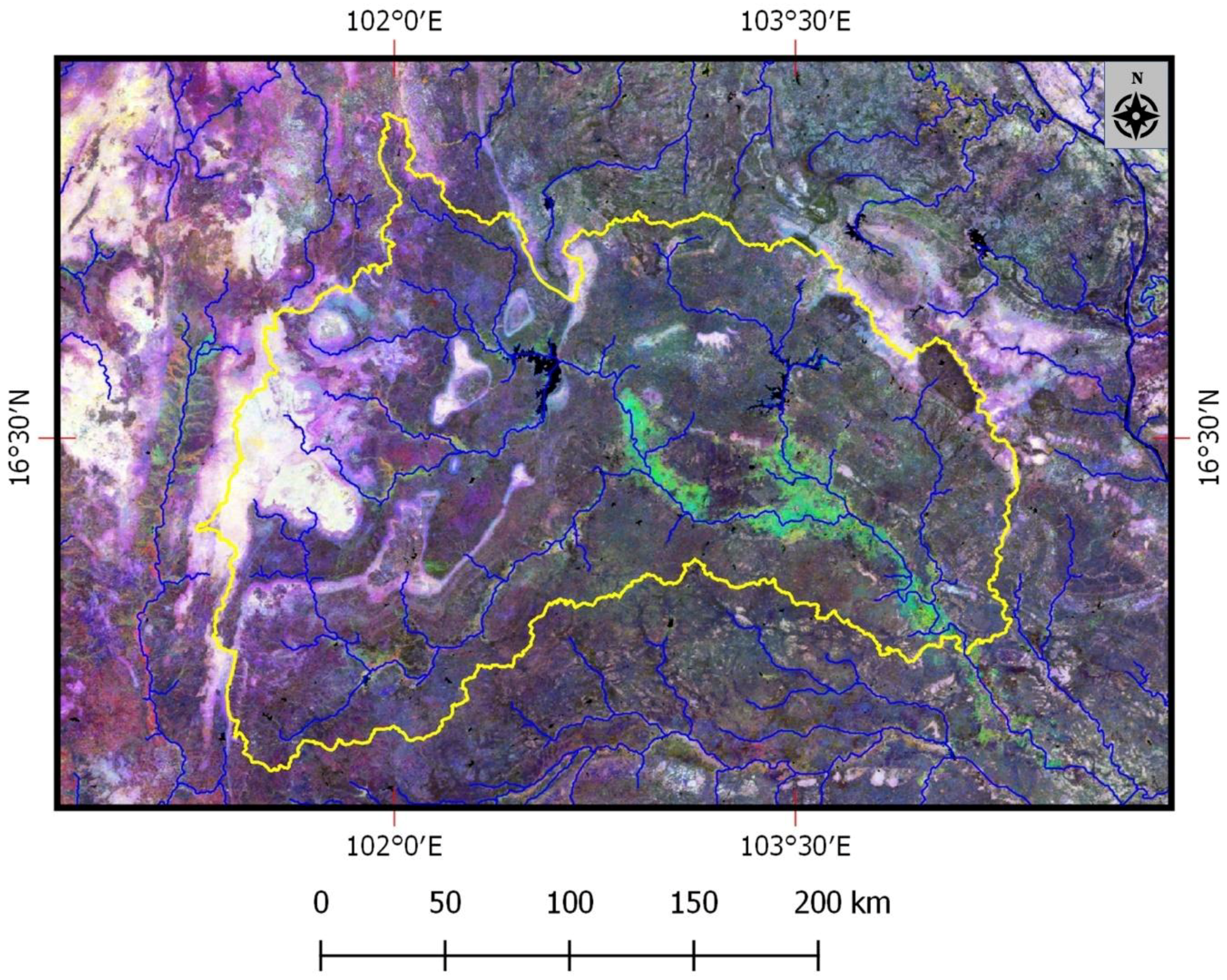
34], was applied to reduce haze effects of each utilized Landsat data set. In the tropics, it is common for even during the dry season that atmospheric contamination effects can occur, and such effects tend to be more evident in the shorter visible wavebands. Such contamination can hinder the production of viable LULC classifications. Consequently, each Landsat data set was subset to include only the red, near infrared, and two short wave infrared bands as a precursor to LULC image classification. Each Landsat scene was then stitched together into a mosaic covering the study area. The preprocessed Landsat mosaic was then assessed for quality assurance (
Figure 6).
2.4. LULC Mapping
Unsupervised and supervised classification methods were both used to process MODIS NDVI and Landsat multispectral data into the needed LULC map of the study area. The unsupervised method was primary technique used for LULC classification. MODIS 32-day NDVI data for 2010 was used to classify regionally evident natural forest and agricultural cover types that exhibited unique vegetation greenness phenology either for the dry season or across a given calendar year. The Landsat mosaic was used to classify locally common but regionally-scarce LULC types that were too fine scaled for detection with MODIS qkm NDVI data.
The LULC classification process began with open water areas being mapped using the MODIS 32-day NDVI data stack for 2010 by (1) extracting the minimum value NDVI considering all 12 dates and (2) using a spatial model to apply a threshold range of NDVI values 1 through 101 to remove all apparent water dominated areas on the minimum value NDVI. The resulting water mask was used to derive a land NDVI data stack. The latter was subjected to a series of unsupervised classifications to map regionally evident agriculture and forest LULC types.
ERDAS Imagine software was used to derive all unsupervised classifications, using an ISODATA clustering routine. The classification parameters were setup as follows. (1) The convergence level to 99.95 percent, (2) the total number of iterations to 100, (3) means initialization along the principal axis, and (4) scaling range using the auto option. In addition, the number of clusters per classification run was set according to the purpose of the classification (e.g., whether the classification was for the whole or a subset of the map area or for a subset of targeted LULC classes).
For unsupervised classifications of study area LULC based on MODIS NDVI data, each cluster class was assessed by comparison to available reference data and then assigned to the apparent predominant LULC class. Reference data for cluster class assessment and LULC class assignment included Landsat RGB multispectral image displays, MODIS NDVI temporal data stacks, Google Map and Bing aerial/satellite high resolution imagery, and assorted reference data from the MRC. The latter included a land cover map for 2010 [
13]; 1997 LULC map with class descriptions [
9], 2010 survey data points, and field photography [
35]; and crop calendars [
36]. The Bing and Google Map imagery were viewed using QGIS software and its OpenLayers plugin [
29]. Some LULC classes (e.g., classes with specific vegetation greenness phenology) required consideration of specific reference data (e.g., 2010 MODIS monthly NDVI data stacks). In some cases, geo-tagged field photography resident to Google Map was also considered.
Although used as a reference, the 2010 land cover map from the MRC [
13] was not produced for aiding the SWAT model and does not include certain LULC classes (e.g., double-cropped rice) that are needed for optimizing SWAT modeling results for applicable LMB SBs 1–8. Other available LULC maps of the LMB region were also not used for this project because they did not include agricultural types needed for optimizing LMB SWAT. The mentioned MRC “2010” land cover map does not distinguish between single and double cropped rice agriculture types, which is regarded as suboptimal for the LMB SWAT models.
The “land” NDVI stack was next applied to produce an unsupervised classification containing 30 cluster classes. The latter was evaluated to identify clusters that were either agriculture or forest dominated. This classification was then recoded to derive two preliminary masks, including one each for apparent agriculture and forest areas. The masks were then used to subset the land NDVI stack into a NDVI stack for agriculture and another for forest. Each of these were then subject to a reclassification process known as cluster busting [
21]. In doing so, Isodata unsupervised clustering was performed independently on agriculture and forest specific NDVI data stacks. The cluster busting process was used to reduce classification confusion for the agriculture and forests occurring in the study area.
The NDVI data for the agricultural areas was used to produce an ISODATA unsupervised classification with 24 total cluster classes. Each of the cluster classes was then assessed and assigned to the apparent predominant LULC class. To aid identification of single versus double-cropped rice areas, an analyst assessed the signatures of each agricultural cluster class that included generation of cluster class specific mean NDVI profiles. In the reclassification of agricultural areas, most of the cluster classes pertained to specific regionally evident agricultural types, including single cropped rice, double-cropped rice, and mixed annual crops that were not rice. A few of the cluster classes (4 total) pertained to forest dominated areas. A lookup table was then developed to recode cluster classes to LULC categories.
MODIS NDVI-based reclassification of the forested areas required a different approach because MODIS NDVIs for mountainous forests had some occasional atmospheric contamination during the rainy season months. Unfortunately, these artifacts persisted even after the data was temporally processed with TSPT. Given the natural forests were to be classified according to deciduousness that typically occurs during the dry season [
37], only dry season NDVI data was used to refine the forest classifications, which included MODIS 32-day NDVI for 32-day dates 1–4 and 10–12. This subset of dates enabled an unsupervised cluster classification of forests that was more visibly effective compared to what could be derived using all 12 dates.
Consequently, the forest 2010 dry season NDVI data stack was used with ISODATA clustering to derive a classification of 16 cluster classes. These were then analyzed using reference data and recoded into LULC types that included four types of forest according to deciduousness level and another related shrubland class that includes mixtures of very young forest regeneration and abandoned, old fallow former agricultural areas.
After preprocessing described earlier, the Landsat mosaic (
Figure 6) was employed to classify additional LULC types that were less regionally common and/or finer scaled compared to MODIS qkm NDVI data. LULC classes mapped with Landsat data included water, barren, urban, bamboo scrub/forest, and industrial forest plantation patches. Unsupervised classification via ISODATA clustering was used to derive these products, though Area of Interest (AOI) vector polygons were also used in some cases to either isolate areas with targeted LULC types or else to reduce classification errors. Initially, the Landsat mosaic was subjected to unsupervised ISODATA clustering with the output containing 40 cluster classes. While some of the cluster classes were associated with the targeted LULC types, additional classification refinement was performed for each Landsat-based LULC class prior to integrating into the final LULC map. More information on mapping of specific LULC classes from Landsat data is given below.
Each LULC class mapped with Landsat 30 m data was recoded into a binary map in which pixels representing the targeted class were set to 100. Afterwards, each 30 m binary map was spatially averaged 8 by 8 pixels with the ERDAS Imagine Degrade function, resulting in a 240-m map indicating the relative fractional abundance of the targeted LULC type. A LULC class specific threshold was then applied to derive a final map of each targeted LULC type. Water, urban, and industrial forest plantation areas were mapped when the per pixel fractional abundance of the targeted LULC type equaled or exceeded 25 percent. Barren and bamboo forest areas where included on the final LUC map when their per pixel fractional abundance equaled 50 percent or more. The water, urban, and IFP classes were assigned a lower fractional abundance threshold because they tended to occur in finer scaled patches that would have been eliminated otherwise. The fractional abundance thresholds were set to a higher value (50%+) for the bamboo forest and barren areas because these types in the study area appeared to primarily occur as larger patches relative to the more frequently finer scaled water, urban, and IFP patches.
The cluster classes representing water were recoded into a binary map that was then used as a mask to isolate Landsat reflectance data for water areas. The latter data was then used to derive an unsupervised classification of 20 cluster classes of which 16 pertained to predominantly water areas. The latter was recoded into a 1 class binary map of water set to a DN of 100 that was then spatially averaged to a 240 m spatial resolution.
The 40-class wall to wall cluster map also contained two clusters that included areas with industrial forest plantations (IFP). Most of the IFP areas were in a highly green state on the Landsat mosaic and thus easy to visualize. The IFP clusters were recoded into a binary map to a DN of 100 that was then spatially averaged to 240 m and edited with AOIs to reduce classification errors.
Urban areas were mapped with Landsat data by initially using AOIs to isolate and subset Landsat data with commonly occurring urban development. The subset imagery was then subjected to an unsupervised classification that contained 30 cluster classes of which four were predominantly urban. The signatures from the unsupervised classification were then input into a maximum likelihood supervised classification routine, along with the entire Landsat mosaic, to produce a wall to wall classification. The urban classes for the latter were recoded into binary urban map to a DN of 100 that was then subjected to an error reduction routine. Errors due to bright bare soil in agricultural areas were reduced by using a spatial model that regarded urban areas to be those mapped by Landsat that also had an annual 2010 MODIS 32-day peak NDVI of less than 160 but greater than or equal to 106.
Bamboo scrub/forest areas were then classified from the Landsat data, using the initial 40 class unsupervised classification to identify four cluster classes containing bamboo areas. Such scrub/forests have a comparatively unique spectral tone and generally occur in higher elevations amongst broadleaved forest types. These bamboo cluster classes also contained some commission error, which was reduced using screen digitized AOIs to more clearly define locations where such areas typically occur. The bamboo scrub/forest clusters were recoded into a binary map to a DN of 100 that was then spatially averaged to 240 m and edited with additional AOIs to reduce classification errors.
Once the individual LULC classes were mapped, a series of raster GIS-based spatial models within ERDAS Imagine were then constructed and applied sequentially to compile a master final LULC map. Six individual models were used to compile the final LULC map in the following sequential steps that added: (1) MODIS-based agriculture and forest LULC classes; (2) MODIS-based shifting cultivation areas; (3) Landsat-based urban zones; (4) Landsat-based industrial forest plantations; (5) MODIS and Landsat-based open water surfaces; and (6) Landsat-based bamboo scrub/forest patches. The final LULC map was coded according to a standard LULC classification scheme and color table.
The 2010 LULC map from this project was then compared visually to the MRC 1997 LULC map. To facilitate this comparison, the 1997 LULC map were recoded to approximate the 2010 LULC classification scheme, given that the 1997 contained some differently defined LULC classes and contained fewer agricultural LULC classes than the 2010 LULC map.
2.5. Method for LULC Accuracy Assessment
The accuracy assessment for the SB 7 LULC map was performed as described previously [
38,
39]. The work flow for this LULC map accuracy assessment is depicted in
Figure 4. The main goal of the LULC map accuracy assessment was to assess the overall accuracy of the final map. A secondary goal was to provide some basic information on individual LULC class mapping performance, knowing that the total samples per scarce individual LULC class was too small for an in-depth assessment of individual class accuracy. The total sampling samples drawn overall and per class considered in part the resources and time available to do the accuracy assessment.
The random selection of sample locations was also designed to assess performance of LULC classifications within the interior of mapped LULC patches as opposed to edges of patches. In doing so, LULC class sample locations were drawn randomly using a 3 by 3-pixel window in which candidate center pixel was compared to the surrounding 8 pixels. Random sampled pixels were selected for accuracy assessment when (1) the center pixel was the targeted class and (2) most of the pixels (at least 5) in the 3 × 3 window were of the same LULC type as the center pixel in the 3 × 3-pixel window.
Initially the sample design was for a stratified random sample of 250 total pixels that were drawn from the LULC classification using ERDAS Imagine software. The number of samples drawn per LULC class was initially based on the observed class frequency on the final LULC map. In doing so, the sample size allocated to each stratum was proportional to the percent area of the stratum relative to the total mapped area. The number of random samples drawn per class depended in part on the LULC class frequency and map extent, as well as the need when feasible to assess at least 10 sample locations per scarce LULC class (
Table 1).
In drawing the sample, the observed LULC classes on the final map were categorized according to four frequency classes: (1) rare = 0 to 0.5 percent of total mapped area; (2) scarce = 0.5 to 10 percent; (3) moderately common = 10 to 20 percent; and (4) highly common = 20 percent or more. Most of the observed LULC classes were relatively scarce compared to the apparent two most frequent types in the final LULC map for SB 7 (
Table 1). These two most common LULC types together represented about 70 percent of the classified pixels. A few of the LULC classes were rare in occurrence. To help improve information on the agreement of individual scarce classes, additional sample locations were drawn for the scarce classes. Fifteen to 20 sample locations were drawn for each scarce class. Doing so enabled the number of sample locations drawn per class to be either equal to or exceeding what the sample size would have been if the sampling allocation was strictly proportional to class frequency. The randomly drawn number of sample locations per common LULC classes were roughly proportional to class frequency for a total sample size of 250. The rare LULC classes were sampled proportional to the class frequency. A total number of 342 random sample locations were drawn considering all LULC classes.
The sample locations for a given SB once selected were converted from an ERDAS Imagine tabular format to spreadsheet and GIS formats using MS Excel, ArcGIS, and QGIS software. QGIS was used to do assess the apparent LULC class for each drawn sample location. Individual points were displayed in QGIS at a 1:10,000 scale according to sample identification # using a zoom to point function and then compared to reference data discussed in
Section 2.4.
Reference imagery used in the map accuracy assessment included Landsat false color RGB mosaic imagery from the dry season of 2009 to 2011. The date of the Landsat data was considered when interpreting sample locations. Also, the apparent vintage of the Google Map satellite imagery, geo-tagged Google Map field photos, and Bing aerial imagery were assessed to make sure that high spatial resolution imagery showed comparable LULC patterns relative to the vintage of the MODIS and Landsat imagery used to produce the final LULC map. Other reference documentation, such as field survey-based notes and example field photos from the MRC was also used.
The Landsat RGBs were used as a general reference to help distinguish between general cover types (e.g., forest versus agriculture) and certain specific cover types that were visually apparent (e.g., urban, water, and bamboo forests). For some of the LULC types (e.g., agricultural types), other reference data had to be used, such as the higher spatial resolution aerial and satellite imagery resident to either Bing or Google Maps. In most cases, multiple sources of reference data were cross compared to assess the apparent predominant LULC type for each randomly sampled pixel.
To assess LULC class within a given sample pixel, the QGIS grid overlay display function was employed to view a given sample location boundary as a vector outline in relation to reference imagery. This display function was used to assess the predominant LULC class for each sample location. In doing so, the grid was proportioned so that it has the same dimensions as the MODIS pixel (~231.65 by 231.65 m). To center the grid around each sample point, one had to apply offsets in the X and Y direction. A trained analyst interpreted and recorded the apparent LULC for each sample location by comparing the location to reference data and determining the predominant LULC type. In using the grid function, the display map projection was set to the Pseudo Mercator map projection so that the dimensions of the grid could be aligned with the boundary of a given sample MODIS qkm pixel.
The LULC map accuracy assessment for certain LULC classes required use of specific reference data. For example, the assessment of sample locations with apparent agricultural and forest LULC types necessitated consideration of the 32-day MODIS NDVI data to assess phenological greenness characteristics. MODIS data was used to assess vegetation greenness phenology, given it was the only synoptic Earth Observation data available at a high temporal resolution for assessing such conditions. However, Landsat, Bing, and Google Maps image data was also used to help assess such sample locations in a supplemental capacity, along with LULC data (e.g., agricultural crop calendars and LULC class descriptions) from the MRC.
Sample locations of rice agricultural areas were assessed in part using pixel specific 32-day MODIS NDVI profiles for 2010 to determine if such areas were cropped one or two times per year. In doing so, a spectral/temporal profiling plugin for QGIS was used to view NDVI profiles of specific pixels. Landsat data was also employed for assessing agricultural type locations, especially with respect to rice types. Although rare in occurrence, sample locations for apparent shifting cultivation agriculture class were assessed using MODIS monthly NDVI data for dates 12 versus 1 of 2010, along with dry season Landsat data of comparable vintage (to the 2010 MODIS data).
Randomly sampled locations of apparent forest were mainly assessed for deciduousness by considering MODIS monthly NDVI values from the dry season of 2010, including 32-day NDVI dates 1–4 and dates 10–12. Such NDVI data were used to quantify two deciduousness indicator metrics for sampled forested pixels: (1) percent NDVI change comparing the median versus maximum NDVI and (2) percent NDVI change comparing the sum of the three lowest versus sum of the three highest NDVIs. Dry season NDVIs were used because of observed higher noisiness of the NDVIs in mountainous forests during the rainy season. Given the same time of year and location, residual unmasked cloud contaminated NDVIs tend to be lower than cloud free NDVIs and can contribute to suboptimal LULC classifications. Consequently, only dry season NDVI data was used to map the forest LULC classes.
For each applicable sample location, the calculated values for each of the two deciduousness indices were compared to decision rules to determine forest class according to an observed level of deciduousness (
Table 2). The thresholds for the different deciduous forest classes were determined previously by analysis of signatures for each predominantly forest cluster class that were derived from the MODIS NDVI unsupervised classification (described in earlier section on LULC map development).
For each apparent forest sample location, a trained analyst assessed the deciduousness level using two deciduousness indicators. The latter were calculated based on MODIS 32-day NDVI data values observed for each sample location considered to be forest. One of these deciduousness indicators (percent change based on median versus maximum NDVI from MODIS data) was used primarily to estimate deciduousness of each apparent forest sample location. For non-obvious borderline cases, estimates from the second index (change based on sum of the three lowest versus sum of three highest dry season NDVIs) were also considered. In addition, Landsat, Google Maps, and Bing imagery were viewed for each sample location. The use of Landsat, Google, and Bing imagery included consideration of the possibility that there may be temporal decorrelation between such data and the MODIS data. A given form of reference data was considered only if it appeared to be of similar vintage to the data used to construct the 2010 LULC map.
Given the cloud frequencies for the region and availability of cloud-free data, Landsat imagery was used as a secondary data source for assessing forest deciduousness. The Landsat data used for a given year was from a single date acquired during the dry season. As such, the timing of peak deciduousness is not necessarily recorded or else highly apparent on the observed Landsat image data. The deciduousness may be only subtly indicated on a given date of dry season Landsat data, depending on the selected date and whether the dry season was wetter, dryer or normal in nature. Consequently, the employed “single snap shot in time” Landsat data did not always show the full degree of forest deciduousness—only what was evident for the acquired date. In addition, even for the selected “best available” Landsat data sets, clouds and shadows sometimes occluded areas of interest.
Results of a given SB LULC accuracy assessment (e.g., for SB 7) were then summarized into error matrices that were subsequently used to calculate overall agreement as well as individual class agreement in terms of user and producer agreement. For a given classification scheme specificity, the overall agreement was then adjusted for random chance effects via use of the Kappa statistic.
4. Discussion
Most of LULC classes were scarce relative to the overall geographic extent of SB 7 and the two most common LULC classes (single annual rice crops and mixed annual crops other than rice). However, the regionally-scarce classes still represented sizeable areas in terms of mapped hectares and were also sometimes locally common. For example, double-cropped rice and certain native forest types were sometimes common in certain locations but regionally-scarce on the final LULC map.
Based on the accuracy assessment results, the monthly MODIS NDVI data in conjunction with unsupervised classification appeared to useful for mapping the more common permanent agricultural cover types in SB 7, particularly the permanent agriculture classes (i.e., irrigated rice, rainfed rice, and annual crops other than rice such as row crops). This is an improvement in terms of increased agricultural classification scheme specificity compared to the preceding LULC map being used for SWAT modeling—the 1997 map maintained by the MRC. The latter shows all forms of permanent agriculture as one singular class. The SB 7 area does not contain extensive shifting cultivation areas, which are more evident in certain other SBs, such as those in Laos PDR. More research is needed to assess the accuracy of using MODIS monthly NDVI data to classify the shifting cultivation LULC types.
In this study, regionally-scarce in occurrence, shrubland, and forest LULC classes showed variable agreement with reference data. The scrub/shrub and evergreen forest types had user and producer agreements that were either moderately high or high. However, the deciduous forest classes (all deciduous, mixed deciduous/evergreen, and mixed evergreen/deciduous forest types) were more frequently confused with each other than hoped. The MODIS data used in LULC classification showed an improved ability to map forest classes according to its deciduousness level once the deciduous related forest classes were reduced from three to one class.
Deciduous forest LULC classification confusion may be due to multiple factors, including map production and evaluation methods. At the outset of the project, it appeared that deciduous forest could be separated via unsupervised image classification of monthly MODIS NDVI data for a calendar year into deciduous forest, mixed deciduous/evergreen forest, and mixed evergreen/deciduous forest types. Such types are known to occur in Thailand based on descriptions by the authors of a previous paper [
24]. On the full classification scheme LULC map, the three-mapped forest deciduous classes tended to be confused with each other. The method for mapping deciduous forest classes in part considered forest deciduousness in relation to cluster class mean 32-day NDVIs for the dry season months. The cluster class signatures also included variability with respect to mean NDVIs per cluster class that may be a factor contributing to the observed confusion between deciduous forest LULC classes. As a result, additional accuracy assessment of forest LULC classes in other SBs with more frequently occurring forests is desirable.
It is possible that the classification of such forest classes may be improved by additional classification and cluster class signature analysis. Also, the forests in SB 7 were much less frequent in occurrence than the main agricultural types. The agricultural classes in some portions of the study area visibly fragmented some of the forested areas, given also that some of the Khorat plateau area was formerly forest prior to agricultural conversion. It is conceivable that the classification of deciduous forest types could improve in other SBs of the LMB in which there is greater representation and perhaps less fragmentation of such forest types.
The overall agreement of the SB 7 LULC map with reference data improved from 81 to 87% when deciduous forest classes were regrouped from three into one class. Once merged, the single deciduous forest class yielded high user and producer class agreement.
Even with only one deciduous forest class, the use of MODIS dry season 32-day NDVI data was able to map two native forest types (deciduous and evergreen) with moderately high to high levels of agreement to available reference data (with user or producer accuracies ranging from 75 to 90%). The ability to monitor forest deciduousness across multiple dates of the dry season was not feasible with Landsat 5 data, due to the low temporal resolution of and the inconsistent availability of cloud-free data (even during the dry season).
The project’s LULC map at both levels of classification scheme specificity yielded an overall agreement with reference data that exceeded 80%. This amount may be conservatively estimated, given that the scarce LULC types were oversampled relative to their percent occurrence. A good land cover map for a given purpose can be deemed as good or acceptable if it has an overall accuracy greater than or equal to 80 to 85% overall accuracy. The latter is comparable to some land cover mapping products that have specifications for accuracy, such as NOAA Coastal Change Analysis Program (C-CAP) land cover maps with multiple wetland classes for the temperate United States. However, the latter C-CAP maps are from Landsat data and do not include as many agricultural classes, compared to the LULC maps we produced for the LMB region in Southeast Asia.
The use of monthly NDVI data derived from twice daily MODIS data collections helped to classify deciduous versus evergreen forest based on seven dates of monthly NDVI for the dry season months of 2010. From a temporal resolution perspective, it appears that the seven dates of MODIS 32-day data enabled an improved means to classify forest deciduousness over using one or two dates of Landsat data, especially given that the duration of the leaf-off state of deciduous forests in Thailand can vary from 2 to 21 weeks [
37].
Even though the project used dry season Landsat 5 data from 2009 to 2011 for LULC classifications (
Figure 6), the cloud frequency in the study area was a factor in assembling the Landsat mosaic in that there was insufficient cloud free data to compile a “clear view” mosaic just from 2010 data. As a result, dry season data from 2009 to 2011 was used instead. Based on this study, the use of a single date of Landsat data per pixel for classifying forest deciduousness can only produce deciduous and evergreen forest maps relative to the foliar state of the forest at the time of data acquisition. The study area mosaic included portions of six Landsat scenes from three swaths. The mosaic based on scenes from three different years and therefore was less suitable for classifying deciduousness forest types.
Given that forest deciduousness patterns can vary from one year to the next, 2010 dry season MODIS 32-day NDVIs (
Figure 5) was used instead of Landsat data (
Figure 6) for mapping native forest types. Landsat false color imagery was useful as an ancillary data source for aiding the interpretation of relative forest deciduousness in the study area however.
In addition, Landsat data showed utility for mapping some of finer scaled LULC types in the study area that are difficult to map as accurately with MODIS data. For example, the Landsat data was used to map regionally infrequent but locally common LULC types. In this study, regionally-scarce water and urban classes both showed high agreement with the reference data. The water class was derived using both MODIS and Landsat data, while the urban class was mapped entirely from Landsat data. Landsat helped to improve effective mapping of finer scaled water bodies. The rare LULC classes recorded on the final LULC map showed variable levels of agreement with reference data, though the very small sample size and class rarity were factors that impeded the ability to fully assess the accuracy of such LULC classes. Some of the rare LULC classes for SB 7 (e.g., industrial forest plantations and shifting cultivation classes) are more common in other SBs of the LMB. Additional accuracy assessment of the rare LULC classes on the SB 7 map is therefore recommended using LULC maps produced from this project for other SBs in the LMB.
The ability to map the specific land cover types at the MODIS qkm spatial resolution is useful for aiding SWAT LMB hydrologic modeling applications given that (1) it is still more spatially resolute than some other SWAT inputs, such as soils and (2) stream flow and runoff characteristics depend in part on the LULC type, according to US Department of Agriculture (USDA) published runoff curves [
40]. For example, the runoff from forests is much less than that from urban areas dominated by impervious surfaces. In addition, the qkm resolution 2010 LULC map is also at a finer scaled MMU (0.0625 km
2) compared to the MRC LULC map for 1997 (latter with a 0.5 km
2 MMU according to [
9]. Consequently, the finer resolution MMU for the 2010 LULC map tended to enable more smaller sized patches to be more discretely mapped compared to the 1997 LULC map.
The 1997 LULC map only classifies permanent agriculture as single class (
Figure 8), while the 2010 LULC map from our project contains multiple permanent agricultural LULC classes (
Figure 7). Both dates of LULC maps show forests generally occurring in the same locations, though the 1997 LULC map has a few locations with shifting cultivation that have apparently reverted to some form of woody vegetation on the 2010 map (
Figure 9). The latter map shows some urban expansion since 1997 and apparent finer scale definition of water bodies.
Given that the 1997 LULC map includes a single permanent agricultural class, a 2010 versus 1997 LULC change map at the 2010 classification scheme specificity was not possible. However, in terms of future work, it is currently feasible to update the 2010 LULC map computed in this project, given that MODIS and Landsat are both still collecting viable data. Also, alternatives to both MODIS (e.g., VIIRS) and Landsat (e.g., Sentinel-2) currently exist.
The project’s LULC mapping method is mostly based on unsupervised classification techniques. It makes use of some supervised techniques, though mainly in terms of how the unsupervised method is applied. Singular use of the supervised approach can be advantageous if there is enough ground reference data to characterize the spectral variability of the targeted LULC types if one uses multispectral imagery like Landsat as a classification input - or the vegetation greenness variability if one uses a year’s worth of monthly MODIS NDVI as an input to classification. For this study, the supervised method was not used due to insufficient training data to account for the apparent spectral variability for some of the targeted types. Also, the cloud frequency on the Landsat data was problematic for singularly using the supervised method in that there was only cloud free data during part of the dry season. That time of year does not necessarily clearly show where all the targeted LULC types are located. In addition, the MODIS data’s spatial coarseness is a factor impeding the singular use of the supervised method.
5. Conclusions
The project combined use of 2010 MODIS 32-day NDVI and Landsat data from 2009 to 2011 to produce an updated LULC map for SB 7 of the LMB. The final LULC map for this SB yielded high overall agreement with available reference data. The MODIS NDVI data was used to map regionally evident LULC types, including certain agricultural and forest types that had specific vegetation greenness phenology signatures. Such LULC classes could not be mapped using monthly composited Landsat data, given that insufficient cloud free data exist for multiple portions of a given calendar year. The MODIS data used in this study enabled regionally common agricultural LULC classes to be mapped at moderately high to high levels of agreement with reference data. The results indicated that deciduous and evergreen broadleaved forest can classified with MODIS NDVI data at a moderately high to high level of agreement with reference data. The results suggest that MODIS NDVI data in conjunction with image classification techniques was not able to consistently map multiple deciduous forest classes in terms of pure deciduous, mixed deciduous/evergreen, and mixed evergreen/deciduous forest types. However, by combining the three deciduous forest classes into one, the technique was able to map a single class of deciduous forest/scrub with a high level of agreement to reference data.
Landsat data appeared to be effective for mapping certain fine scaled LULC classes that were less detectable on the qkm MODIS NDVI data, including urban and fine scaled waterways. The Landsat data showed some potential for mapping other finer scaled LULC types (e.g., IFP areas) output at the MODIS qkm scale, though additional quantitative accuracy assessment of other SBs is needed to confirm this belief.
The project yielded a new technique for mapping tropical deciduous forest classes that included utilization of forest deciduousness indicators computed from 2010 MODIS 32-day NDVI data. The latter data was useful for viewing per pixel fluctuations in vegetation canopy greenness that occurs during the LMB dry season when forest leaf drop primarily occurs.
The project enabled updated LULC maps to be produced for all eight SBs of the LMB that are currently being analyzed with MRC SWAT hydrologic models. The LULC maps from the project are being used to help SWAT modelers improve predictions of water flow dynamics that in turn is being used for aiding water management and basin planning in the LMB. Updated LULC maps along with soils, terrain, and precipitation maps from the project are being used to generate needed SWAT modeling products [
41,
42,
43]. The LULC maps from the project also provided more specific maps of rice paddies (single- versus double-cropped or rainfed versus irrigated) that are potentially helpful for aiding other basin planning efforts in the LMB, including flood damage monitoring and assessment applications [
44,
45].


