Abstract
Urbanization can affect the ecological processes, local climate and human health in urban areas by changing the vegetation phenology. In the past 20 years, China has experienced rapid urbanization. Thus, it is imperative to understand the impact of urbanization on vegetation phenology in China. In this study, we quantitatively analyzed the impact of urbanization on vegetation phenology at the national and climate zone scales using remotely sensed data. We found that the start of the growing season (SOS) was advanced by approximately 2.4 days (P < 0.01), and the end of the growing season (EOS) was delayed by approximately 0.7 days (P < 0.01) in the urban areas compared to the rural areas. As a result, the growing season length (GSL) was extended by approximately 3.1 days (P < 0.01). The difference in the SOS and GSL between the urban and rural areas increased from 2001 to 2014, with an annual rate of 0.2 days (R2 = 0.39, P < 0.05) and 0.2 days (R2 = 0.31, P < 0.05), respectively. We also found that the impact of urbanization on vegetation phenology varied among different vegetation types at the national and climate zone levels (P < 0.05). The SOS was negatively correlated with land surface temperature (LST), with a correlation coefficient of −0.24 (P < 0.01), and EOS and GSL were positively correlated with LST, with correlation coefficients of 0.56 and 0.44 (P < 0.01), respectively. The improved understanding of the impact of urbanization on vegetation phenology from this study will be of great help for policy-makers in terms of developing relevant strategies to mitigate the negative environmental effects of urbanization in China.
1. Introduction
Vegetation phenology is the study of periodic plant life cycle events and how these events are influenced by interannual variations in climate and other environmental factors [1,2,3,4]. Vegetation phenology was widely investigated to analyze the impact of ecological processes and environmental conditions on terrestrial ecosystems, including impacts on biodiversity, carbon emissions, surface temperature change and land use and land cover changes [5,6,7,8,9]. Changes in vegetation phenology affect ecological processes by altering the cycling of energy, nutrients and water in terrestrial ecosystems [10,11,12]. Thus, studies of vegetation phenology have drawn the global attention.
Human activities, such as the urbanization, are one of the most important factors that change vegetation phenology by affecting climate conditions, soil properties, hydrology and ecosystem processes [13,14,15,16,17,18]. Conversely, changes in vegetation phenology also affect local climate, energy consumption and human health in urban areas [19,20,21,22,23]. Since the Reform and Opening-up, China has experienced rapid urbanization [24,25]. From 1981 to 2012, the urban population in China has increased by more than two times, and the built-up areas have increased by more than five times [26,27]. Therefore, it is of great significance to understand the impact of urbanization on vegetation phenology in China.
Many studies have assessed the impact of urbanization on vegetation phenology. Existing studies have investigated the mechanisms, influential factors and potential impacts of changes in vegetation phenology in urban areas [16,28,29]. In terms of mechanisms, ecological processes and vegetation functional types were examined to understand the impact of urbanization on vegetation phenology [30,31,32]. To assess the influential factors, temperature, moisture, photoperiod and atmospheric compositions were investigated [33,34,35,36,37]. With regard to the consequences of the impact of urbanization on vegetation phenology, studies have assessed ecological processes, human health and economic development [38,39,40,41]. The datasets used in these studies were mainly derived from site-based observations and satellite remote sensing. The quality of site-based observations is relatively high, and the data can be analyzed for specific plants [42,43]. However, site-based observations are limited in the spatial coverage [44]. Remotely sensed datasets have demonstrated their power in investigating the impact of urbanization on vegetation phenology over large areas [2,45,46]. However, earth observation sensor types and data preprocessing models should be chosen cautiously when estimating vegetation phenology [44,47,48,49,50].
Studies on the impact of urbanization on vegetation phenology in China have mainly been conducted at the city scale [28,40]. For example, Zhou et al. [13] analyzed the differences in vegetation phenology among 32 major cities and their surrounding rural areas in China. They found that the start of the growing season (SOS) was advanced by an average of 11.9 days, and the end of the growing season (EOS) was delayed by an average of 5.4 days in urban areas compared to rural areas. Han et al. [51] analyzed the vegetation phenological differences among six cities and their surrounding rural areas in the Yangtze River Delta. They also found that urbanization advanced the SOS, delayed the EOS and extended the growing season length (GSL). Moreover, previous studies have found that the impact of urbanization on vegetation phenology varied across different climate zones [11,52,53,54,55,56]. Since there are multiple climate zones with a wide range of latitudes and complex topographies in China [52,57,58], it is highly necessary to understand the regional differences in urbanization impacts on vegetation phenology in China.
Because of the importance of urbanization impacts on phenology in China and the lack of studies at the national and regional levels, in this study, we investigated the impact of urbanization on vegetation phenology at the national and climate zone scales. The objectives of this study were to: (1) understand the difference in vegetation phenology between urban and rural areas and the variations across climate zones and vegetation types and (2) evaluate the trend of the phenological difference from 2001 to 2014. We also examined the relationship between vegetation phenology and land surface temperature (LST). The remainder of this paper is structured as follows. Section 2 describes the Materials and Methods. The Results and Discussion are reported in Section 3 and Section 4, respectively. The Conclusions are presented in Section 5.
2. Materials and Methods
2.1. Study Area
Our study examined the phenological difference between urban and surrounding rural areas in China (Figure 1). The urban areas were derived from the Defense Meteorological Satellite Program/Operational Linescan System (DMSP/OLS) nighttime light data in 2013 using a cluster-based method that estimated the optimal thresholds of clusters based on their size and the overall nightlight magnitude [59,60]. The urban area was dominated by built-up areas but contained vegetated areas (e.g., crop areas) because the urban extent considered here is the urban boundary, not the area of impervious surface [60,61,62,63]. Following Li et al. [45], we excluded urban clusters smaller than 10 km2 because they were too small to investigate the impact of urbanization on vegetation phenology. Overall, there were more than 1000 urban clusters in China, with a total area of approximately 80,000 km2. The urban areas ranged from 10 km2 to larger than 1700 km2, and the mean value was 77 km2. The average percentage of vegetation among the urban clusters was approximately 59%. Specifically, we divided all urban areas into 11 bins according to the size. The average area of vegetation among the bins ranged from 6 km2 to 388 km2, and the percentage of vegetation pixels to the total pixels in each bin was greater than 50%. Thus, we can assume that there are adequate vegetation pixels in urban areas for the purposes of analysis [44]. The rural extent was determined by keeping its size the same as that of the urban extent [45]. That is, we gradually increased the buffering zone around the initial shape of the urban area until the extent of the surrounding rural area was equal to the corresponding urban area. In rural areas, the area of vegetation was nearly 70,000 km2, accounting for almost 90% of the total rural area (Figure 2).
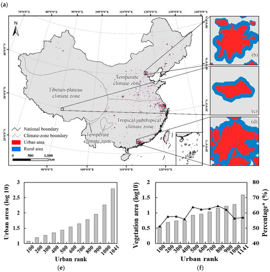
Figure 1.
Urban clusters and rural buffers in (a) China and the three enlarged examples in (b) Beijing; (c) Lhasa, and (d) Guangzhou, which illustrate the extent of the urban clusters; (e) The average size of the urban area in each bin; (f) The average size of the vegetation area in each bin. The percentage is the proportion of the number of vegetation pixels to the total number of pixels in each bin. The unit of area is km2.
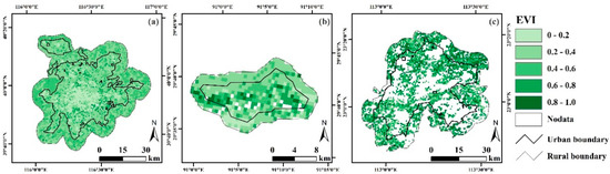
Figure 2.
The EVI values corresponding to the dormancy onset date from the product MCD12Q2 in three enlarged examples to show vegetation configuration. The EVI was the mean value from 2011 to 2014 to mitigate the uncertainty from annual fluctuations. The enlarged examples are (a) Beijing in the temperate climate zone; (b) Lhasa in the Tibetan-plateau climate zone and (c) Guangzhou in the tropical/subtropical climate zone. Please refer to Figure 1 for their locations in China.
We divided China into three climate zones, i.e., the tropical/subtropical, temperate and Tibetan-plateau climate zones, as described in Wang et al. [52]. Among the three climate zones, the annual accumulated temperature (i.e., the annual sum of daily mean temperature when it was equal to or larger than 10 °C) in the tropical/subtropical climate zone was above 8000 °C, while the annual accumulated temperature in the temperate and Tibetan-plateau climate zones were below 8000 °C and 2000 °C, respectively. Specifically, there were 343 urban clusters in the tropical/subtropical climate zone, and the average size of the urban areas was approximately 120 km2. The number of urban clusters in the temperate and Tibetan-plateau climate zones were 688 and 10, respectively. The average sizes of the urban areas in the temperate and Tibetan-plateau climate zones were 56 km2 and 45 km2, respectively.
2.2. Data
The main data used in this study include the urban area, vegetation phenology, land cover, LST and auxiliary data. The urban area data for China had a spatial resolution of 1 km and were produced by Zhou et al. [59,60]. The data can accurately reflect the urban pattern at a large scale. The average Kappa and average overall accuracy of the data are greater than 0.54 and 93%, respectively. We resampled the urban area data from a 1-km resolution to a 500-m using a nearest neighbor approach to make the data consistent with other Moderate Resolution Imaging Spectroradiometer (MODIS) products [45].
The vegetation phenology data were derived from the MODIS land cover dynamic product MCD12Q2 at a resolution of 500 m [64]. The data were radiometrically calibrated, georeferenced and corrected for atmospheric effects. These data have been validated with field observations [65] and have been widely used in previous studies [66].
The land cover data were derived from the MODIS product MCD12Q1 at a resolution of 500 m [67]. The vegetation types of the International Geosphere Biosphere Programme (IGBP) in MCD12Q1 include evergreen forest (EF), deciduous forest (DF), mixed forest (MF), shrubland (SB), grassland (GL), cropland (CP), and natural mosaic [68].
The LST data were derived from the MODIS product MYD11A2 with a spatial resolution of 1 km and errors within 1 K. The product was built from the clear-sky observations at 1:30 AM and 1:30 PM local solar times using the generalized split-window algorithm [69,70]. Similarly, we resampled the data to a 500-m resolution using the nearest neighbor approach. The auxiliary data, including the administrative boundaries in China at a scale of 1:4,000,000, were collected from the National Geomatics Center of China (http://ngcc.sbsm.gov.cn).
2.3. Methods
The method for assessing the impact of urbanization on vegetation phenology using remotely sensed data is illustrated in Figure 3. First, we analyzed the difference in vegetation phenology between the urban and rural areas. Then, we evaluated the trend of the vegetation phenological differences from 2001 to 2014. Finally, we investigated the variations in the urbanization impacts on vegetation phenology across vegetation types as well as the relationship between the vegetation phenology and LST.
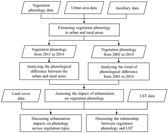
Figure 3.
The flow chart of the method proposed in this study.
2.3.1. Phenology Indicators
Following Li et al. [45], we examined the impact of urbanization on vegetation phenology using the SOS, EOS and GSL as phenological indicators. The SOS and EOS indicate the dates of onset and the end of photosynthetic activity, respectively. The GSL is defined as the difference between the EOS and SOS. Meanwhile, we excluded the extreme values in the vegetation phenology data. That is, we excluded the pixels with an SOS before the 30th day of the year or later than the 180th day of the year. Similarly, the EOS was constrained between the 240th and 350th day of the year. We extracted three phenology indicators in the urban and rural areas in China from 2001 to 2014.
2.3.2. Differences in Phenology between the Urban and Rural Areas
The ratio of vegetation phenology between the urban areas and their corresponding rural areas in China was examined using a regression analysis as shown below:
where Pub is the mean value of the vegetation phenology indicators (i.e., SOS, EOS and GSL) from 2011 to 2014 in the urban areas. Pr represents the mean value of the vegetation phenology indicators from 2011 to 2014 in the corresponding rural areas, and a indicates the relationship of phenology between the urban and rural areas. If a is larger than 1, it indicates that the SOS or EOS in the urban areas have a delay with respect to the values in the rural areas, or the GSL is extended. If a is smaller than 1, it indicates that the SOS or EOS in the urban areas will be advanced, or the GSL will be shortened. We confirmed the statistical significance of the regression model using t-test. That is, the phenological difference between the urban and corresponding rural areas was significant in this study when the P was lower than 0.05. We used the mean value of the phenology indicators from 2011 to 2014 to mitigate the uncertainty from annual fluctuations. We also calculated the difference in phenology between the urban and its corresponding rural area to show the specific impacts of urbanization.
2.3.3. Trend of the Phenological Differences between the Urban and Rural Areas
We analyzed the trend of the phenological differences between the urban and corresponding rural areas from 2001 to 2014 using a linear regression analysis, as shown below:
where y is the regression value of the phenological difference between the urban and corresponding rural areas in the year t. An increase in indicates that the phenological difference increases over time, and a decrease indicates that the difference decreases over time. b is the slope of the regression line, which represents the annual change rate of the phenological difference. c represents the intercept. In addition, we performed the significance test for the regression equation, as indicated by the p values. Specifically, the phenological difference between the urban and corresponding rural areas experienced a significant change when p was lower than 0.05.
2.3.4. Relationship between Vegetation Phenology and LST
We analyzed the relationship between vegetation phenology and LST by pooling all urban and rural areas using Pearson’s correlation coefficient, as shown below:
where R is the correlation coefficient between vegetation phenology and LST. Xi is the vegetation indicator in the urban or rural area i, and Yi is the LST in the corresponding urban or rural area. The LST was represented by the mean value from 2011 to 2014, which was consistent with the vegetation phenology indicator, for mitigating the impact of annual fluctuations. The significance test was performed for the correlation coefficient as indicated by t-test. Specifically, the vegetation phenology was significantly correlated with the LST when p was lower than 0.05.
3. Results
3.1. Differences in Phenology between the Urban and Rural Areas
The three phenology indicators (i.e., SOS, EOS and GSL) showed a distinct difference between the urban and rural areas in China. Overall, urban areas were associated with an earlier SOS and a later EOS, resulting in a longer GSL (Figure 4). The SOS occurred earlier in the urban areas, as suggested by the regression slope smaller than 1 (R2 = 0.78). For the EOS, the slope of the regression line was greater than 1, suggesting a delayed EOS in the urban areas (R2 = 0.70). The slope of the regression line for the GSL was greater than 1, suggesting an extended GSL for the urban areas (R2 = 0.73). Specifically, in the urban areas, the average SOS was approximately 102, and the average EOS and GSL were approximately 298 and 196, respectively. In the rural areas, the average SOS was 104, and the average EOS and GSL were 297 and 193, respectively. On average, the SOS was advanced by 2.4 days (P < 0.01), while the EOS was delayed by 0.7 days (P < 0.01) in the urban areas. Consequently, the GSL was extended by 3.1 days (P < 0.01) (Table 1).
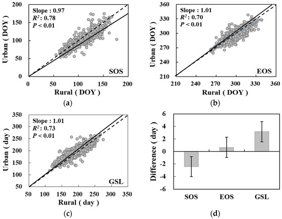
Figure 4.
The relationship of vegetation phenology indicators of (a) SOS, (b) EOS and (c) GSL between urban areas and their corresponding rural areas; (d) The difference in phenology between the urban and its corresponding rural areas. The error bars represent the standard error.

Table 1.
The impact of urbanization on vegetation phenology.
The phenological difference between the urban and rural areas varied by climate zone (Table 1). Urban areas had an earlier SOS, later EOS and longer GSL compared to the rural areas in the Tibetan-plateau climate zone and the temperate climate zone, which was in line with the trend at the national scale. Specifically, in the Tibetan-plateau climate zone, the average SOS was advanced by 7.5 days (P < 0.01), while the EOS was delayed by 3.0 days (P < 0.01). Consequently, the GSL was extended by 10.5 days in the urban areas (P < 0.01). In the temperate climate zone, the SOS was advanced by 3.6 days (P < 0.01), while the EOS was delayed by 1.8 days (P < 0.01). As a result, the GSL was extended by 5.4 days in the urban areas (P < 0.01). In contrast, urbanization had a significant influence only on the EOS in the tropical/subtropical climate zone. The EOS was advanced by 1.9 days.
3.2. Trend of the Phenological Differences between the Urban and Rural Areas
The difference in the SOS and GSL between urban and rural areas increased at the national scale from 2001 to 2014 (Figure 5). The difference in the SOS increased from 1.0 days in 2001 to 2.3 days in 2014, with an annual rate of 0.2 days (R2 = 0.39, P < 0.05). The difference in the GSL increased from 2.1 days in 2001 to 3.3 days in 2014, with an annual rate of 0.2 days (R2 = 0.31, P < 0.05). The difference in the EOS did not show a significant trend over time.
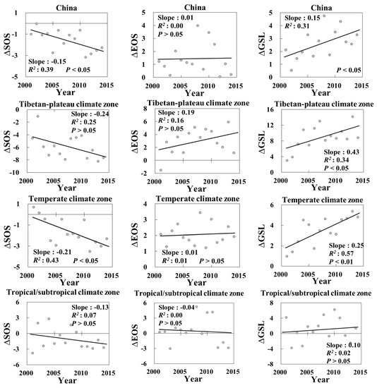
Figure 5.
The trend of the phenological differences between the urban and rural areas from 2001 to 2014 (unit: day).
In the Tibetan-plateau climate zone, the difference in the GSL between the urban and rural areas increased significantly. The difference in the GSL between the urban and rural areas increased from 3.0 days in 2001 to 8.8 days in 2014, with an annual rate of 0.4 days (R2 = 0.34, P < 0.05). In the temperate climate zone, the difference in the SOS and GSL between the urban and rural areas increased significantly. The difference in the SOS increased from −0.7 days in 2001 to 2.3 days in 2014, with an annual rate of 0.2 days (R2 = 0.43, P < 0.05). The difference in the GSL increased in the urban areas from 1.0 days in 2001 to 7.8 days in 2014, with an annual rate of 0.3 days (R2 = 0.57, P < 0.01). The difference in the vegetation phenology between the urban and rural areas did not change significantly in the tropical/subtropical climate zone.
4. Discussion
4.1. Impacts of Urbanization on Phenology across Vegetation Types
The impact of urbanization on phenology varies across vegetation types [45]. Therefore, we further analyzed the variations in the impact of urbanization on phenology in China at the national and climate zone levels (Figure 6 and Table 2). We calculated the phenological differences between the urban and the corresponding rural areas with the same dominant vegetation type (i.e., the type that covered the largest area). We presumed that the phenological differences between the urban and the corresponding rural areas were mainly derived from the dominant vegetation type [44]. We found that there were significant differences in the SOS between the urban and rural areas in shrublands, grasslands and croplands (P < 0.01). Specifically, the SOS in shrublands, grasslands and croplands were advanced by 10.0, 5.7 and 1.4 days, respectively. The EOS had significant differences between the urban and rural areas in shrublands and grasslands (P < 0.05) and were delayed by 4.3 and 2.8, respectively. For the GSL, there were significant differences between the urban and rural areas in shrublands, grasslands and croplands (P < 0.01). Among the three vegetation types, the GSL showed the largest increase in shrublands, which was 14.4 days. The GSL in grasslands and croplands increased by 8.9 days and 1.6 days, respectively. These findings were consistent with those of previous studies, which found that the impacts of urbanization on phenology were the greatest in shrublands and grasslands [28]. The EOS in croplands did not exhibit a significant change because of the impact of human management [20].
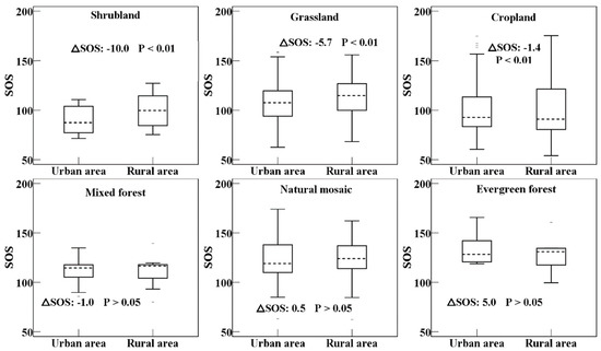
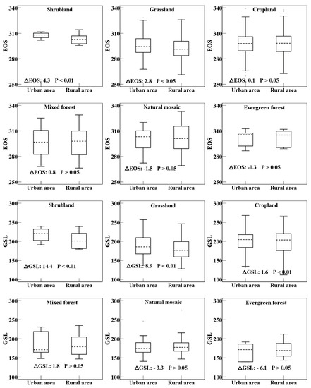
Figure 6.
The differences in the phenology of different vegetation types between urban and rural areas. △SOS, △EOS and △GSL refer to the mean value of the SOS, EOS, and GSL in urban areas minus the mean value in rural areas, respectively. We used t-test to calculate the significance of the phenological differences.
Table 2.
The impact of urbanization on phenology across vegetation types (unit: day).
The impact of urbanization on different vegetation types also varied among climate zones (Table 2). The phenology showed significant differences between the urban and rural areas in most vegetation types in the Tibetan-plateau climate zone and the temperate climate zone (P < 0.05). Specifically, in the Tibetan-plateau climate zone, the SOS, EOS and GSL had significant differences between the urban and rural areas in shrublands and grasslands (P < 0.05). In the temperate climate zone, the SOS had significant differences between the urban and rural areas in shrublands, grasslands, croplands and natural mosaic (P < 0.05). The urban-rural differences of the EOS and GSL in natural mosaic were also significant (P < 0.05). The difference in the EOS and GSL was significantly in only croplands in the tropical/subtropical climate zone (P < 0.05).
4.2. Relationship between Phenology and LST
Temperature is one of the most important factors affecting vegetation phenology. It is recognized that urbanization can cause significant differences in temperature between urban and rural areas, which is known as the urban heat island [19,71,72,73]. Thus, following the method used by Zhou et al. [13], we further examined the relationship between vegetation phenology and LST at multiple scales (Table 3). We found that an earlier SOS, a later EOS and a longer GSL were associated with an increase in the LST, which is in line with the results of previous studies [13]. Specifically, the SOS was negatively correlated with the LST, and the correlation coefficient was −0.24 (P < 0.01). The EOS and GSL were positively correlated with the LST, and the correlation coefficients were 0.56 and 0.44 (P < 0.01), respectively. Therefore, we inferred that urbanization could affect vegetation phenology by changing the LST.
Table 3.
Relationship between LST and phenology in urban and rural areas.
The relationship between vegetation phenology and LST in the Tibetan-plateau climate zone and the temperate climate zone was consistent with the relationship at the national scale. In the Tibetan-plateau climate zone, the correlation coefficient between the SOS and LST was −0.44 (P < 0.05). The correlation coefficients between the EOS and LST and between the GSL and LST were 0.64 (P < 0.01) and 0.55 (P < 0.05), respectively. In the temperate climate zone, the correlation coefficient between the SOS and LST was −0.80 (P < 0.01). The correlation coefficients between the EOS and LST and between the GSL and LST were 0.58 (P < 0.01) and 0.81 (P < 0.01), respectively. The increase in the LST was associated with a later EOS and SOS and a shorter GSL in the tropical/subtropical climate zone. The possible reason explaining this result is that the temperature is not the major factor limiting vegetation growth in this climate zone that has a high temperature [64,65].
5. Conclusions
This study investigated the impact of urbanization on vegetation phenology at the national and climate zone scales using remotely sensed data. Specifically, we analyzed the differences in vegetation phenology between the urban and rural areas and the trend of the phenological differences. We found that vegetation phenology showed a distinct difference between the urban and rural areas in China. The phenological differences between the urban and rural areas increased from 2001 to 2014.
We also investigated the impact of urbanization across vegetation types and the relationship between vegetation phenology and LST. The results indicated that the impact of urbanization on vegetation phenology varied among different vegetation types at the national and climate zone levels. An earlier SOS, a later EOS and a longer GSL were associated with the increase in LST.
It is of great significance to choose an appropriate data preprocessing model when estimating vegetation phenology. The data we used underwent a smoothing process based on the fitted logistic function and performed well in most areas of China [65,74]. However, there are still other data preprocessing models that have a better accuracy in some specific study areas [44,75]. Thus, special attention should be paid to the applicability of the data preprocessing models in a given study area. In addition, the earth observation sensor types can also affect the estimation of vegetation phenology [47,48]. The differences and similarities of urbanization impacts on vegetation phenology can be explored by using data from different earth observation sensors in the future.
The findings from this study are of great use for policymakers and managers in urban and regional planning. Our results can benefit from more comprehensive datasets. First, the spatial resolution of the remotely sensed data is 500 m, which makes it difficult to adequately capture the impact of urbanization in small urban areas. Second, we only analyzed the relationships between LST and vegetation phenology. However, other factors still affect vegetation phenology. In the future, high spatial resolution phenology data can play an important role in investigating the impact of urbanization on vegetation phenology [76,77,78]. An improved understanding of the driving mechanisms and factors (e.g., precipitation and soil condition) of the impact of urbanization on vegetation phenology is still needed [20,28].
Author Contributions
Y.Z. conceived and supervised the research topic; Q.R. performed the experiments, analyzed the data and wrote the paper. Y.Z., C.H. and Q.H. contributed to the manuscript revisions.
Funding
This work was supported in part by the National Natural Science Foundation of China (grant no. 41621061). The research was also supported by the Fundamental Research Funds for the Central Universities and the project from State Key Laboratory of Earth Surface Processes and Resource Ecology, China (grant no. 2017-KF-09).
Acknowledgments
We express our gratitude to anonymous reviewers and editors for their professional comments and suggestions.
Conflicts of Interest
The authors declare no conflict of interest.
References
- Chen, X.; Wang, D.; Chen, J.; Wang, C.; Shen, M. The mixed pixel effect in land surface phenology: A simulation study. Remote Sens. Environ. 2018, 211, 338–344. [Google Scholar] [CrossRef]
- White, M.A.; de Beurs, K.M.; Didan, K.; Inouye, D.W.; Richardson, A.D.; Jensen, O.P.; O’Keefe, J.; Zhang, G.; Nemani, R.R.; van Leeuwen, W.J.D.; et al. Intercomparison, interpretation, and assessment of spring phenology in North America estimated from remote sensing for 1982–2006. Glob. Chang. Biol. 2009, 15, 2335–2359. [Google Scholar] [CrossRef]
- Linderholm, H.W. Growing season changes in the last century. Agric. For. Meteorol. 2006, 137, 1–14. [Google Scholar] [CrossRef]
- Badeck, F.W.; Bondeau, A.; Bottcher, K.; Doktor, D.; Lucht, W.; Schaber, J.; Sitch, S. Responses of spring phenology to climate change. New Phytol. 2004, 162, 295–309. [Google Scholar] [CrossRef]
- Da Silva, A.; Valcu, M.; Kempenaers, B. Light pollution alters the phenology of dawn and dusk singing in common European songbirds. Philos. Trans. R. Soc. Lond. Ser. B Biol. Sci. 2015, 370. [Google Scholar] [CrossRef] [PubMed]
- Dahlin, K.M.; Fisher, R.A.; Lawrence, P.J. Environmental drivers of drought deciduous phenology in the Community Land Model. Biogeosciences 2015, 12, 5061–5074. [Google Scholar] [CrossRef]
- Lu, P.; Yu, Q.; Liu, J.; Lee, X. Advance of tree-flowering dates in response to urban climate change. Agric. For. Meteorol. 2006, 138, 120–131. [Google Scholar] [CrossRef]
- Seto, K.C.; Guneralp, B.; Hutyra, L.R. Global forecasts of urban expansion to 2030 and direct impacts on biodiversity and carbon pools. Proc. Natl. Acad. Sci. USA 2012, 109, 16083–16088. [Google Scholar] [CrossRef] [PubMed]
- Tang, H.; Li, Z.; Zhu, Z.; Chen, B.; Zhang, B.; Xin, X. Variability and climate change trend in vegetation phenology of recent decades in the Greater Khingan Mountain area, Northeastern China. Remote Sens. 2015, 7, 11914–11932. [Google Scholar] [CrossRef]
- Keenan, T.F.; Gray, J.; Friedl, M.A.; Toomey, M.; Bohrer, G.; Hollinger, D.Y.; Munger, J.W.; O’Keefe, J.; Schmid, H.P.; Wing, I.S.; et al. Net carbon uptake has increased through warming-induced changes in temperate forest phenology. Nat. Clim. Chang. 2014, 4, 598–604. [Google Scholar] [CrossRef]
- Richardson, A.D.; Keenan, T.F.; Migliavacca, M.; Ryu, Y.; Sonnentag, O.; Toomey, M. Climate change, phenology, and phenological control of vegetation feedbacks to the climate system. Agric. For. Meteorol. 2013, 169, 156–173. [Google Scholar] [CrossRef]
- Piao, S.; Ciais, P.; Friedlingstein, P.; Peylin, P.; Reichstein, M.; Luyssaert, S.; Margolis, H.; Fang, J.; Barr, A.; Chen, A.; et al. Net carbon dioxide losses of northern ecosystems in response to autumn warming. Nature 2008, 451, 49–52. [Google Scholar] [CrossRef] [PubMed]
- Zhou, D.; Zhao, S.; Zhang, L.; Liu, S. Remotely sensed assessment of urbanization effects on vegetation phenology in China’s 32 major cities. Remote Sens. Environ. 2016, 176, 272–281. [Google Scholar] [CrossRef]
- Tang, J.; Körner, C.; Muraoka, H.; Piao, S.; Shen, M.; Thackeray, S.J.; Yang, X. Emerging opportunities and challenges in phenology: A review. Ecosphere 2016, 7, 1–17. [Google Scholar] [CrossRef]
- Liang, S.; Shi, P.; Li, H. Urban spring phenology in the middle temperate zone of China: Dynamics and influence factors. Int. J. Biometeorol. 2016, 60, 531–544. [Google Scholar] [CrossRef] [PubMed]
- Wu, J. Urban ecology and sustainability: The state-of-the-science and future directions. Landsc. Urban Plan. 2014, 125, 209–221. [Google Scholar] [CrossRef]
- Grimm, N.B.; Faeth, S.H.; Golubiewski, N.E.; Redman, C.L.; Wu, J.; Bai, X.; Briggs, J.M. Global change and the ecology of cities. Science 2008, 319, 756–760. [Google Scholar] [CrossRef] [PubMed]
- Qiu, T.; Song, C.; Li, J. Impacts of urbanization on vegetation phenology over the past three decades in Shanghai, China. Remote Sens. 2017, 9, 970. [Google Scholar] [CrossRef]
- Bounoua, L.; Zhang, P.; Mostovoy, G.; Thome, K.; Masek, J.; Imhoff, M.; Shepherd, M.; Quattrochi, D.; Santanello, J.; Silva, J.; et al. Impact of urbanization on US surface climate. Environ. Res. Lett. 2015, 10, 084010. [Google Scholar] [CrossRef]
- Buyantuyev, A.; Wu, J. Urbanization diversifies land surface phenology in arid environments: Interactions among vegetation, climatic variation, and land use pattern in the Phoenix metropolitan region, USA. Landsc. Urban Plan. 2012, 105, 149–159. [Google Scholar] [CrossRef]
- Cong, N.; Piao, S.; Chen, A.; Wang, X.; Lin, X.; Chen, S.; Han, S.; Zhou, G.; Zhang, X. Spring vegetation green-up date in China inferred from SPOT NDVI data: A multiple model analysis. Agric. For. Meteorol. 2012, 165, 104–113. [Google Scholar] [CrossRef]
- Cecchi, L.; D’Amato, G.; Ayres, J.G.; Galan, C.; Forastiere, F.; Forsberg, B.; Gerritsen, J.; Nunes, C.; Behrendt, H.; Akdis, C.; et al. Projections of the effects of climate change on allergic asthma: The contribution of aerobiology. Allergy 2010, 65, 1073–1081. [Google Scholar] [CrossRef] [PubMed]
- Van Vliet, A.J.H.; Overeem, A.; De Groot, R.S.; Jacobs, A.F.G.; Spieksma, F.T.M. The influence of temperature and climate change on the timing of pollen release in the Netherlands. Int. J. Climatol. 2002, 22, 1757–1767. [Google Scholar] [CrossRef]
- Bai, X.; Shi, P.; Liu, Y. Society: Realizing China’s urban dream. Nature 2014, 509, 158–160. [Google Scholar] [CrossRef] [PubMed]
- He, C.; Gao, B.; Huang, Q.; Ma, Q.; Dou, Y. Environmental degradation in the urban areas of China: Evidence from multi-source remote sensing data. Remote Sens. Environ. 2017, 193, 65–75. [Google Scholar] [CrossRef]
- National Bureau of Statistics of China. China Statistical Yearbook; China Statistics Press: Beijing, China, 2013; ISBN 978-7-5037-6963-4.
- Ministry of Housing and Urban-Rural Development PRC. China Urban Construction Statistical Yearbook 2011; China Planning Press: Beijing, China, 2012; ISBN 978-7-80242-909-3.
- Jochner, S.; Menzel, A. Urban phenological studies—Past, present, future. Environ. Pollut. 2015, 203, 250–261. [Google Scholar] [CrossRef] [PubMed]
- Neil, K.; Wu, J. Effects of urbanization on plant flowering phenology: A review. Urban Ecosyst. 2006, 9, 243–257. [Google Scholar] [CrossRef]
- Hepper, F.N. Phenological records of English garden plants in Leeds (Yorkshire) and Richmond (Surrey) from 1946 to 2002. An analysis relating to global warming. Biodivers. Conserv. 2003, 12, 2503–2520. [Google Scholar] [CrossRef]
- Traidl-Hoffmann, C.; Kasche, A.; Menzel, A.; Jakob, T.; Thiel, M.; Ring, J.; Behrendt, H. Impact of pollen on human health: More than allergen carriers? Int. Arch. Allergy Immunol. 2003, 131, 1–13. [Google Scholar] [CrossRef] [PubMed]
- Fitter, A.H.; Fitter, R.S. Rapid changes in flowering time in British plants. Science 2002, 296, 1689–1691. [Google Scholar] [CrossRef] [PubMed]
- Mimet, A.; Pellissier, V.; Quenol, H.; Aguejdad, R.; Dubreuil, V.; Roze, F. Urbanisation induces early flowering: Evidence from Platanus acerifolia and Prunus cerasus. Int. J. Biometeorol. 2009, 53, 287–298. [Google Scholar] [CrossRef] [PubMed]
- Zhang, X.Y.; Friedl, M.A.; Schaaf, C.B.; Strahler, A.H. Climate controls on vegetation phenological patterns in northern mid- and high latitudes inferred from MODIS data. Glob. Chang. Biol. 2004, 10, 1133–1145. [Google Scholar] [CrossRef]
- Primack, D.; Imbres, C.; Primack, R.B.; Millerrushing, A.J.; Tredici, P.D. Herbarium specimens demonstrate earlier flowering times in response to warming in Boston. Am. J. Bot. 2004, 91, 1260–1264. [Google Scholar] [CrossRef] [PubMed]
- Franklin, K.A.; Whitelam, G.C. Light signals, phytochromes and cross-talk with other environmental cues. J. Exp. Bot. 2004, 55, 271–276. [Google Scholar] [CrossRef] [PubMed]
- Shen, M.; Tang, Y.; Chen, J.; Zhu, X.; Zheng, Y. Influences of temperature and precipitation before the growing season on spring phenology in grasslands of the central and eastern Qinghai-Tibetan Plateau. Agric. For. Meteorol. 2011, 151, 1711–1722. [Google Scholar] [CrossRef]
- Kudo, G.; Nishikawa, Y.; Kasagi, T.; Kosuge, S. Does seed production of spring ephemerals decrease when spring comes early? Ecol. Res. 2010, 19, 255–259. [Google Scholar] [CrossRef]
- Ziello, C.; Böck, A.; Estrella, N.; Ankerst, D.; Menzel, A. First flowering of wind-pollinated species with the greatest phenological advances in Europe. Ecography 2012, 35, 1017–1023. [Google Scholar] [CrossRef]
- Jochner, S.C.; Sparks, T.H.; Estrella, N.; Menzel, A. The influence of altitude and urbanisation on trends and mean dates in phenology (1980–2009). Int. J. Biometeorol. 2012, 56, 387–394. [Google Scholar] [CrossRef] [PubMed]
- Xin, Q.; Broich, M.; Suyker, A.E.; Yu, L.; Gong, P. Multi-scale evaluation of light use efficiency in MODIS gross primary productivity for croplands in the Midwestern United States. Agric. For. Meteorol. 2015, 201, 111–119. [Google Scholar] [CrossRef]
- Luo, Z.; Sun, O.J.; Ge, Q.; Xu, W.; Zheng, J. Phenological responses of plants to climate change in an urban environment. Ecol. Res. 2006, 22, 507–514. [Google Scholar] [CrossRef]
- Jochner, S.; Caffarra, A.; Menzel, A. Can spatial data substitute temporal data in phenological modelling? A survey using birch flowering. Tree Physiol. 2013, 33, 1256–1268. [Google Scholar] [CrossRef] [PubMed]
- Atkinson, P.M.; Jeganathan, C.; Dash, J.; Atzberger, C. Inter-comparison of four models for smoothing satellite sensor time-series data to estimate vegetation phenology. Remote Sens. Environ. 2012, 123, 400–417. [Google Scholar] [CrossRef]
- Li, X.; Zhou, Y.; Asrar, G.R.; Mao, J.; Li, X.; Li, W. Response of vegetation phenology to urbanization in the conterminous United States. Glob. Chang. Biol. 2017, 23, 2818–2830. [Google Scholar] [CrossRef] [PubMed]
- Gazal, R.; White, M.A.; Gillies, R.; Rodemaker, E.L.I.; Sparrow, E.; Gordon, L. GLOBE students, teachers, and scientists demonstrate variable differences between urban and rural leaf phenology. Glob. Chang. Biol. 2008, 14, 1568–1580. [Google Scholar] [CrossRef]
- Atzberger, C.; Klisch, A.; Mattiuzzi, M.; Vuolo, F. Phenological Metrics Derived over the European Continent from NDVI3g Data and MODIS Time Series. Remote Sens. 2014, 6, 257–284. [Google Scholar] [CrossRef]
- Van Leeuwen, W.J.D.; Orr, B.J.; Marsh, S.E.; Herrmann, S.M. Multi-sensor NDVI data continuity: Uncertainties and implications for vegetation monitoring applications. Remote Sens. Environ. 2006, 100, 67–81. [Google Scholar] [CrossRef]
- Beck, P.S.A.; Atzberger, C.; Høgda, K.A.; Johansen, B.; Skidmore, A.K. Improved monitoring of vegetation dynamics at very high latitudes: A new method using MODIS NDVI. Remote Sens. Environ. 2006, 100, 321–334. [Google Scholar] [CrossRef]
- Meroni, M.; Atzberger, C.; Vancutsem, C.; Gobron, N.; Baret, F.; Lacaze, R.; Eerens, H.; Leo, O. Evaluation of Agreement Between Space Remote Sensing SPOT-VEGETATION fAPAR Time Series. IEEE Transa. Geosci. Remote Sens. 2013, 51, 1951–1962. [Google Scholar] [CrossRef]
- Han, G.; Xu, J. Land surface phenology and land surface temperature changes along an urban-rural gradient in Yangtze River Delta, China. Environ. Manag. 2013, 52, 234–249. [Google Scholar] [CrossRef] [PubMed]
- Wang, J.; Zuo, W. Geographic Atlas of China; SinoMaps Press: Beijing, China, 2009; ISBN 9787503152337. [Google Scholar]
- Zhang, S.; Tao, F. Modeling the response of rice phenology to climate change and variability in different climatic zones: Comparisons of five models. Eur. J. Agron. 2013, 45, 165–176. [Google Scholar] [CrossRef]
- Rishmawi, K.; Prince, S.; Xue, Y. Vegetation Responses to Climate Variability in the Northern Arid to Sub-Humid Zones of Sub-Saharan Africa. Remote Sens. 2016, 8, 910. [Google Scholar] [CrossRef]
- Machar, I.; Vlckova, V.; Bucek, A.; Vozenilek, V.; Salek, L.; Jerabkova, L. Modelling of Climate Conditions in Forest Vegetation Zones as a Support Tool for Forest Management Strategy in European Beech Dominated Forests. Forests 2017, 8, 82. [Google Scholar] [CrossRef]
- Luo, Z.; Yu, S. Spatiotemporal Variability of Land Surface Phenology in China from 2001–2014. Remote Sens. 2017, 9, 65. [Google Scholar] [CrossRef]
- Wang, P.X.; Wang, B.; Cheng, H.; Fasullo, J.; Guo, Z.; Kiefer, T.; Liu, Z. The global monsoon across time scales: Mechanisms and outstanding issues. Earth-Sci. Rev. 2017, 174, 84–121. [Google Scholar] [CrossRef]
- Piao, S.; Ciais, P.; Huang, Y.; Shen, Z.; Peng, S.; Li, J.; Zhou, L.; Liu, H.; Ma, Y.; Ding, Y.; et al. The impacts of climate change on water resources and agriculture in China. Nature 2010, 467, 43–51. [Google Scholar] [CrossRef] [PubMed]
- Zhou, Y.; Smith, S.J.; Elvidge, C.D.; Zhao, K.; Thomson, A.; Imhoff, M. A cluster-based method to map urban area from DMSP/OLS nightlights. Remote Sens. Environ. 2014, 147, 173–185. [Google Scholar] [CrossRef]
- Zhou, Y.; Smith, S.J.; Zhao, K.; Imhoff, M.; Thomson, A.; Bond-Lamberty, B.; Asrar, G.R.; Zhang, X.; He, C.; Elvidge, C.D. A global map of urban extent from nightlights. Environ. Res. Lett. 2015, 10, 054011. [Google Scholar] [CrossRef]
- Zhou, Y.; Li, X.; Asrar, G.R.; Smith, S.J.; Imhoff, M. A global record of annual urban dynamics (1992–2013) from nighttime lights. Remote Sens. Environ. 2018, 219, 206–220. [Google Scholar] [CrossRef]
- He, C.Y.; Liu, Z.F.; Tian, J.; Ma, Q. Urban expansion dynamics and natural habitat loss in China: A multiscale landscape perspective. Glob. Chang. Biol. 2014, 20, 2886–2902. [Google Scholar] [CrossRef] [PubMed]
- Liu, Z.F.; He, C.Y.; Zhou, Y.Y.; Wu, J.G. How much of the world’s land has been urbanized, really? A hierarchical framework for avoiding confusion. Landsc. Ecol. 2014, 29, 763–771. [Google Scholar] [CrossRef]
- Ganguly, S.; Friedl, M.A.; Tan, B.; Zhang, X.; Verma, M. Land surface phenology from MODIS: Characterization of the Collection 5 global land cover dynamics product. Remote Sens. Environ. 2010, 114, 1805–1816. [Google Scholar] [CrossRef]
- Zhang, X.; Friedl, M.A.; Schaaf, C.B. Global vegetation phenology from Moderate Resolution Imaging Spectroradiometer (MODIS): Evaluation of global patterns and comparison with in situ measurements. J. Geophys. Res. Biogeosci. 2006, 111. [Google Scholar] [CrossRef]
- Zhang, X.; Friedl, M.A.; Schaaf, C.B.; Strahler, A.H.; Schneider, A. The footprint of urban climates on vegetation phenology. Geophys. Res. Lett. 2004, 31. [Google Scholar] [CrossRef]
- Belward, A.S.; Estes, J.E.; Kline, K.D. The IGBP-DIS global 1-km land-cover data set DISCover: A project overview. Photogramm. Eng. Remote Sens. 1999, 65, 1013–1020. [Google Scholar]
- Svirejeva-Hopkins, A.; Schellnhuber, H.J. Modelling carbon dynamics from urban land conversion: Fundamental model of city in relation to a local carbon cycle. Carbon Balanc. Manag. 2006, 1, 8. [Google Scholar] [CrossRef] [PubMed]
- Wan, Z. New refinements and validation of the MODIS Land-Surface Temperature/Emissivity products. Remote Sens. Environ. 2008, 112, 265–279. [Google Scholar] [CrossRef]
- Wan, Z.; Dozier, J. A generalized split-window algorithm for retrieving land-surface temperature from space. IEEE Trans. Geosci. Remote Sens. 1996, 34, 892–905. [Google Scholar] [CrossRef]
- Li, X.; Zhou, Y.; Asrar, G.R.; Imhoff, M.; Li, X. The surface urban heat island response to urban expansion: A panel analysis for the conterminous United States. Sci. Total Environ. 2017, 605–606, 426–435. [Google Scholar] [CrossRef] [PubMed]
- Clinton, N.; Gong, P. MODIS detected surface urban heat islands and sinks: Global locations and controls. Remote Sens. Environ. 2013, 134, 294–304. [Google Scholar] [CrossRef]
- Krehbiel, C.; Zhang, X.; Henebry, G. Impacts of Thermal Time on Land Surface Phenology in Urban Areas. Remote Sens. 2017, 9, 499. [Google Scholar] [CrossRef]
- Zhang, X.; Friedl, M.A.; Schaaf, C.B.; Strahler, A.H.; Hodges, J.C.F.; Gao, F.; Reed, B.C.; Huete, A. Monitoring vegetation phenology using MODIS. Remote Sens. Environ. 2003, 84, 471–475. [Google Scholar] [CrossRef]
- Atzberger, C.; Eilers, P.H.C. Evaluating the effectiveness of smoothing algorithms in the absence of ground reference measurements. Int. J. Remote Sens. 2011, 32, 3689–3709. [Google Scholar] [CrossRef]
- Li, X.; Zhou, Y.; Asrar, G.R.; Meng, L. Characterizing spatiotemporal dynamics in phenology of urban ecosystems based on Landsat data. Sci. Total Environ. 2017, 605–606, 721–734. [Google Scholar] [CrossRef] [PubMed]
- Melaas, E.K.; Friedl, M.A.; Zhu, Z. Detecting interannual variation in deciduous broadleaf forest phenology using Landsat TM/ETM+ data. Remote Sens. Environ. 2013, 132, 176–185. [Google Scholar] [CrossRef]
- Fisher, J.; Mustard, J.; Vadeboncoeur, M. Green leaf phenology at Landsat resolution: Scaling from the field to the satellite. Remote Sens. Environ. 2006, 100, 265–279. [Google Scholar] [CrossRef]


© 2018 by the authors. Licensee MDPI, Basel, Switzerland. This article is an open access article distributed under the terms and conditions of the Creative Commons Attribution (CC BY) license (http://creativecommons.org/licenses/by/4.0/).