Sparse Cost Volume for Efficient Stereo Matching

 , ,
, ,
Abstract
:
1. Introduction
2. Related Work
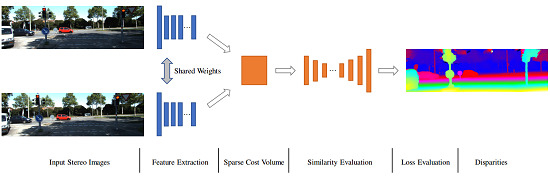
3. Method
3.1. Feature Extraction
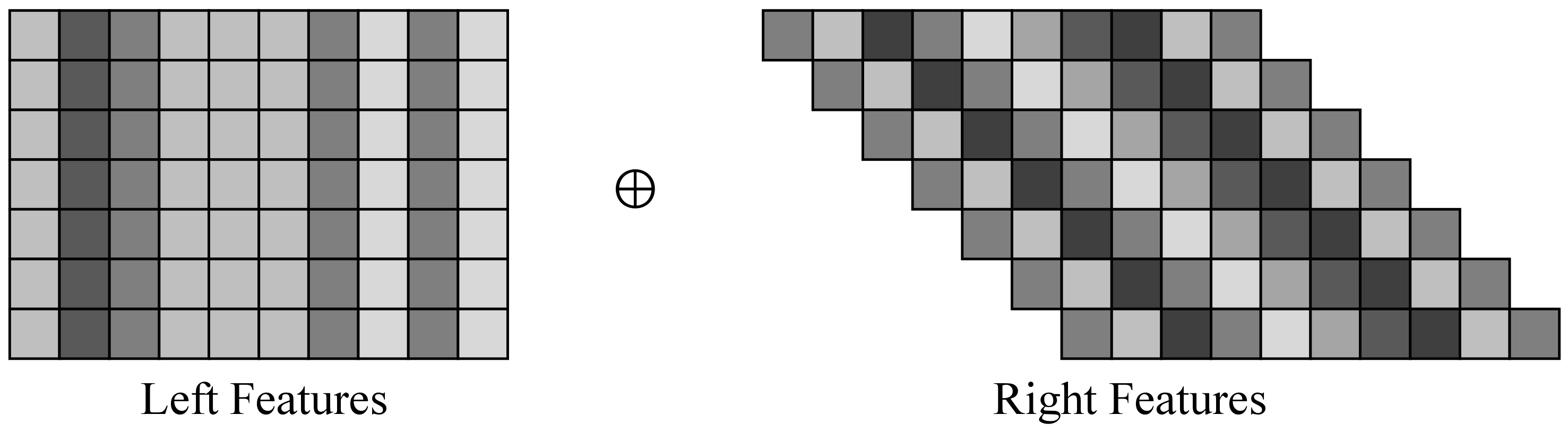
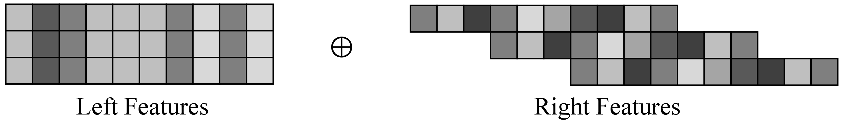
3.2. Sparse Cost Volume Construction
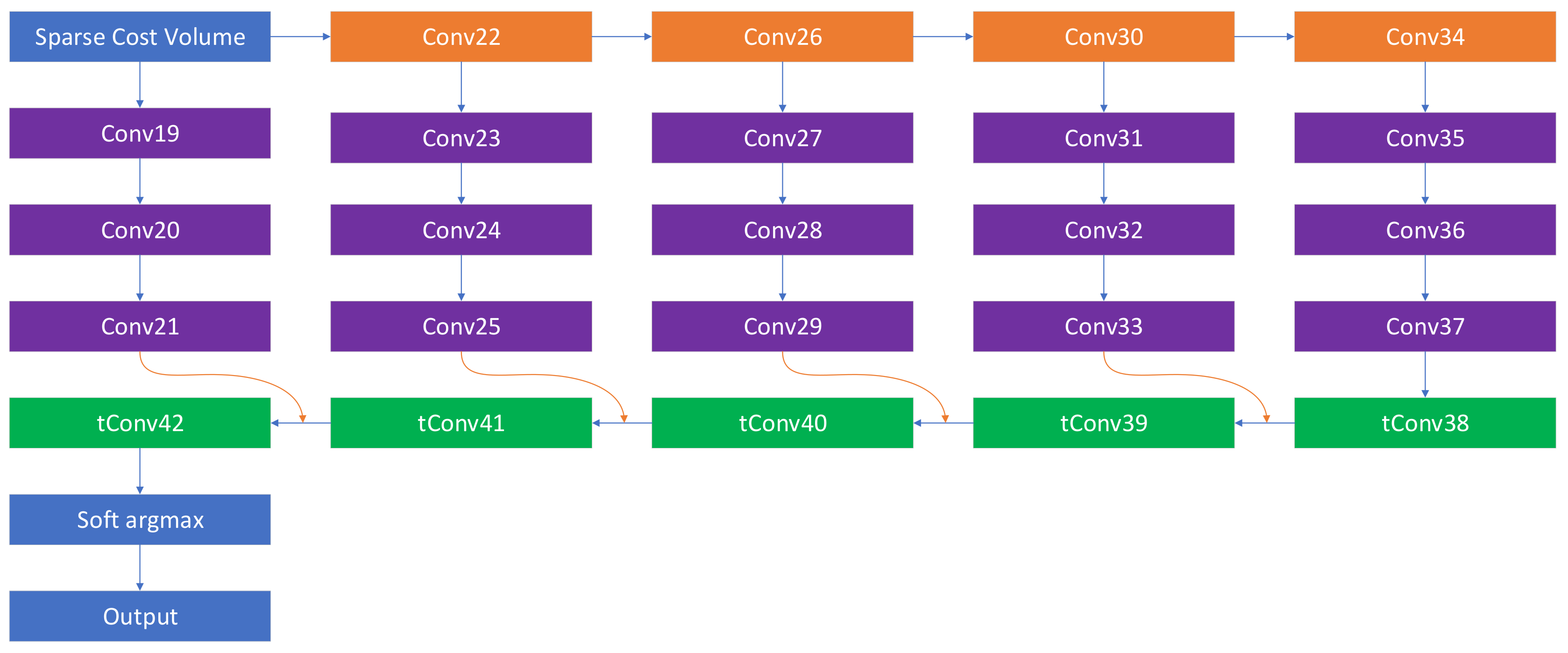
3.3. Similarity Evaluation
3.4. Loss Function
3.5. Weight Normalization
4. Experiments
4.1. Implementation Detail
4.2. Computational Efficiency
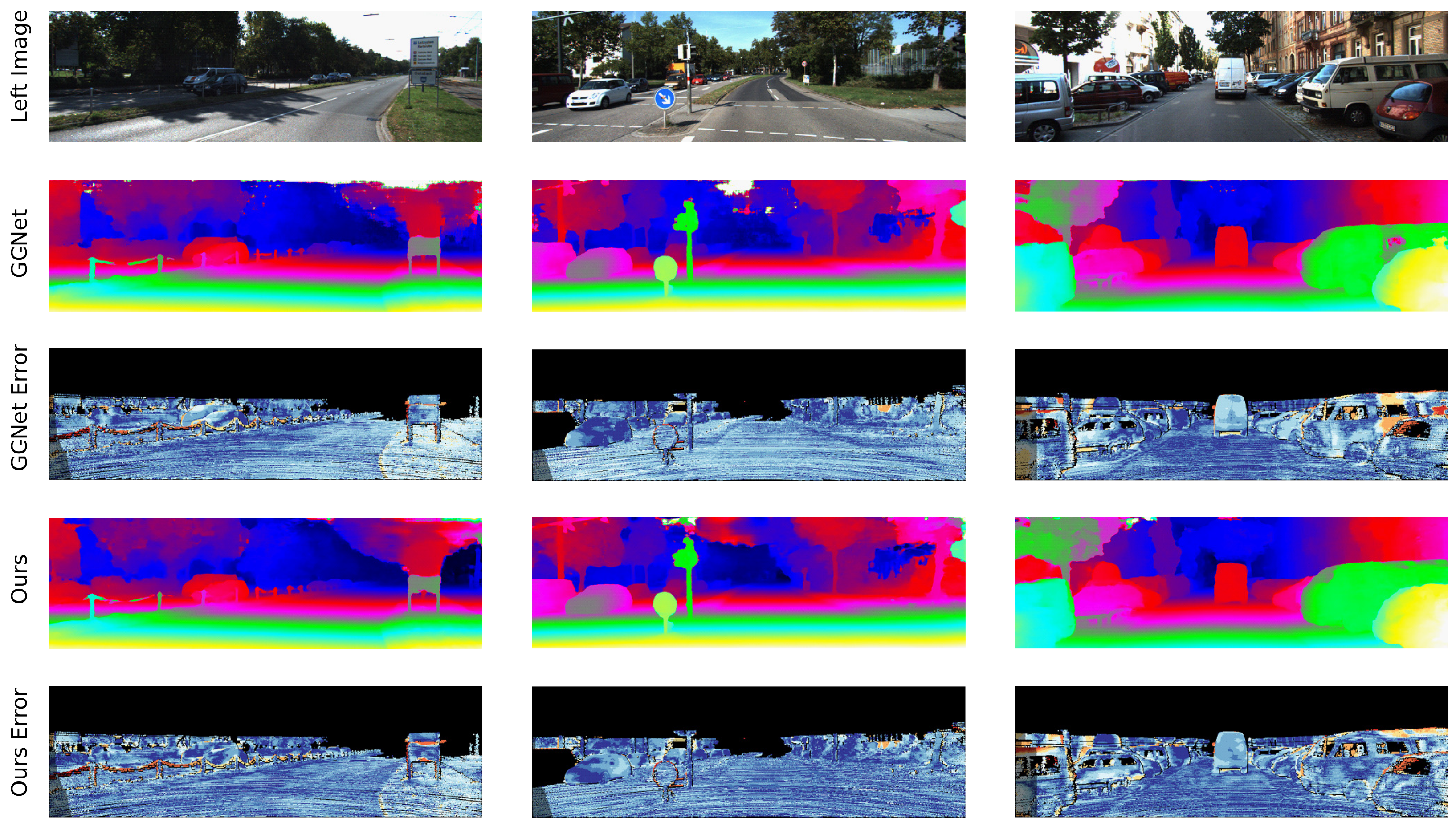
4.3. Benchmark Results
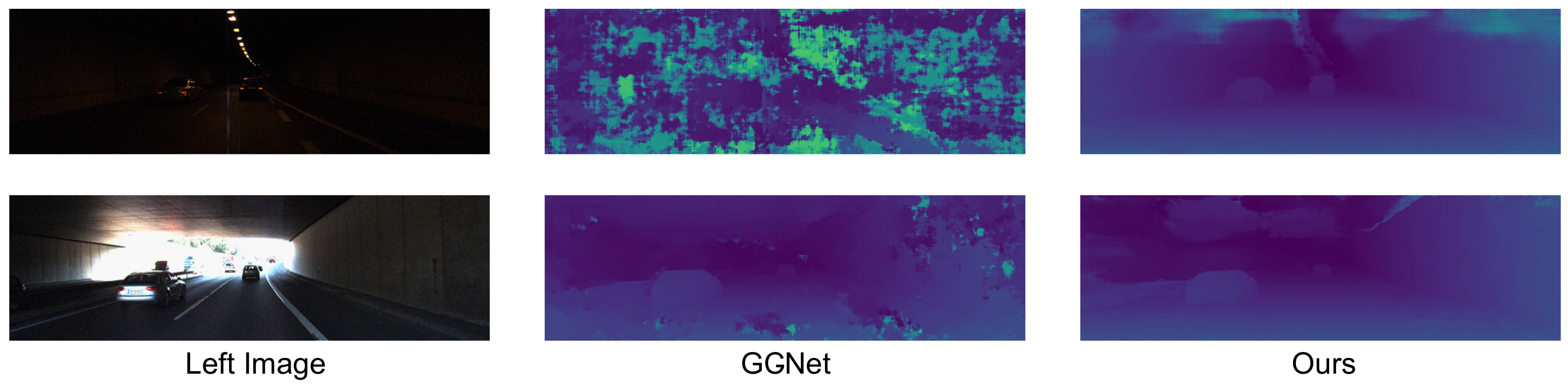
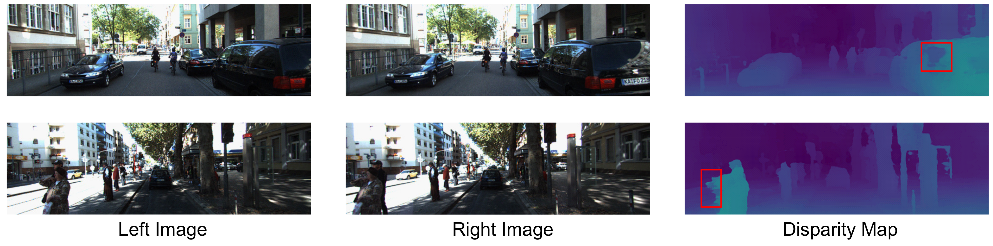
4.4. Discussions
5. Conclusions
Author Contributions
Funding
Conflicts of Interest
References
- Newcombe, R.A.; Izadi, S.; Hilliges, O.; Molyneaux, D.; Kim, D.; Davison, A.J.; Kohi, P.; Shotton, J.; Hodges, S.; Fitzgibbon, A. KinectFusion: Real-time dense surface mapping and tracking. In Proceedings of the 10th IEEE international symposium on IEEE Mixed and augmented reality (ISMAR), Basel, Switzerland, 26–29 October 2011; pp. 127–136. [Google Scholar]
- Helmer, S.; Lowe, D. Using stereo for object recognition. In Proceedings of the 2010 IEEE International Conference on Robotics and Automation, Anchorage, AK, USA, 3–7 May 2010; pp. 3121–3127. [Google Scholar]
- Howard, A. Real-time stereo visual odometry for autonomous ground vehicles. In Proceedings of the IEEE/RSJ 2008 International Conference on Intelligent RObots and Systems, Nice, France, 22–26 September 2008; pp. 3946–3952. [Google Scholar]
- Scharstein, D.; Szeliski, R. A taxonomy and evaluation of dense two-frame stereo correspondence algorithms. Int. J. Comput. Vis. 2002, 47, 7–42. [Google Scholar] [CrossRef]
- Zbontar, J.; LeCun, Y. Computing the stereo matching cost with a convolutional neural network. In Proceedings of the IEEE Conference on Computer Vision and Pattern Recognition, Boston, MA, USA, 7–12 June 2015; pp. 1592–1599. [Google Scholar]
- Luo, W.; Schwing, A.G.; Urtasun, R. Efficient deep learning for stereo matching. In Proceedings of the IEEE Conference on Computer Vision and Pattern Recognition, Las Vegas, NV, USA, 26 June–1 July 2016; pp. 5695–5703. [Google Scholar]
- Mayer, N.; Ilg, E.; Hausser, P.; Fischer, P.; Cremers, D.; Dosovitskiy, A.; Brox, T. A large dataset to train convolutional networks for disparity, optical flow, and scene flow estimation. In Proceedings of the IEEE Conference on Computer Vision and Pattern Recognition, Las Vegas, NV, USA, 26 June–1 July 2016; pp. 4040–4048. [Google Scholar]
- Kendall, A.; Martirosyan, H.; Dasgupta, S.; Henry, P.; Kennedy, R.; Bachrach, A.; Bry, A. End-to-end learning of geometry and context for deep stereo regression. arXiv, 2017; arXiv:1703.04309. [Google Scholar]
- Salimans, T.; Kingma, D.P. Weight normalization: A simple reparameterization to accelerate training of deep neural networks. In Advances in Neural Information Processing Systems; MIT Press: Cambridge, MA, USA, 2016; pp. 901–909. [Google Scholar]
- Zagoruyko, S.; Komodakis, N. Learning to compare image patches via convolutional neural networks. In Proceedings of the IEEE Conference on Computer Vision and Pattern Recognition, Boston, MA, USA, 7–12 June 2015; pp. 4353–4361. [Google Scholar]
- Seki, A.; Pollefeys, M. Sgm-nets: Semi-global matching with neural networks. In Proceedings of the 2017 IEEE Conference on Computer Vision and Pattern Recognition Workshops (CVPRW), Honolulu, HI, USA, 1 July 2017; pp. 21–26. [Google Scholar]
- Gidaris, S.; Komodakis, N. Detect, replace, refine: Deep structured prediction for pixel wise labeling. In Proceedings of the IEEE Conference on Computer Vision and Pattern Recognition, Honolulu, HI, USA, 21–26 July 2017; pp. 5248–5257. [Google Scholar]
- Pang, J.; Sun, W.; Ren, J.; Yang, C.; Yan, Q. Cascade residual learning: A two-stage convolutional neural network for stereo matching. In Proceedings of the International Conference on Computer Vision-Workshop on Geometry Meets Deep Learning (ICCVW 2017), Venice, Italy, 28 October 2017; Volume 3. [Google Scholar]
- Jie, Z.; Wang, P.; Ling, Y.; Zhao, B.; Wei, Y.; Feng, J.; Liu, W. Left-Right Comparative Recurrent Model for Stereo Matching. arXiv, 2018; arXiv:1804.00796. [Google Scholar]
- Liang, Z.; Feng, Y.; Guo, Y.; Liu, H. Learning for Disparity Estimation through Feature Constancy. arXiv, 2017; arXiv:1712.01039. [Google Scholar]
- Chang, J.R.; Chen, Y.S. Pyramid Stereo Matching Network. arXiv, 2018; arXiv:1803.08669. [Google Scholar]
- Wang, L.; Jin, H.; Yang, R. Search Space Reduction for MRF Stereo. European Conference on Computer Vision; Springer: Berlin, Germany, 2008; pp. 576–588. [Google Scholar]
- Veksler, O. Reducing Search Space for Stereo Correspondence with Graph Cuts. In Proceedings of the British Machine Vision Conference (BMVC), Citeseer, Edinburgh, UK, 4–7 September 2006; pp. 709–718. [Google Scholar]
- Geiger, A.; Roser, M.; Urtasun, R. Efficient large-scale stereo matching. In Computer Vision–ACCV 2010; Springer: Berlin, Germany, 2010; pp. 25–38. [Google Scholar]
- Gürbüz, Y.Z.; Alatan, A.A.; Çığla, C. Sparse recursive cost aggregation towards O (1) complexity local stereo matching. In Proceedings of the 23rd Signal Processing and Communications Applications Conference (SIU), Malatya, Turkey, 16–19 May 2015; pp. 2290–2293. [Google Scholar]
- Khamis, S.; Fanello, S.; Rhemann, C.; Kowdle, A.; Valentin, J.; Izadi, S. StereoNet: Guided Hierarchical Refinement for Real-Time Edge-Aware Depth Prediction. In Proceedings of the European Conference on Computer Vision (ECCV), Munich, Germany, 8–14 September 2018; pp. 573–590. [Google Scholar]
- Huang, G.; Liu, Z.; Weinberger, K.Q.; van der Maaten, L. Densely connected convolutional networks. In Proceedings of the IEEE Conference on Computer Vision and Pattern Recognition, Honolulu, HI, USA, 21–26 July 2017; Volume 1, p. 3. [Google Scholar]
- He, K.; Zhang, X.; Ren, S.; Sun, J. Deep residual learning for image recognition. In Proceedings of the IEEE Conference on Computer Vision and Pattern Recognition, Las Vegas, NV, USA, 26 June–1 July 2016; pp. 770–778. [Google Scholar]
- Dosovitskiy, A.; Fischer, P.; Ilg, E.; Hausser, P.; Hazirbas, C.; Golkov, V.; van der Smagt, P.; Cremers, D.; Brox, T. Flownet: Learning optical flow with convolutional networks. In Proceedings of the IEEE International Conference on Computer Vision, Washington, DC, USA, 7–13 December 2015; pp. 2758–2766. [Google Scholar]
- Ilg, E.; Mayer, N.; Saikia, T.; Keuper, M.; Dosovitskiy, A.; Brox, T. Flownet 2.0: Evolution of optical flow estimation with deep networks. In Proceedings of the IEEE Conference on Computer Vision and Pattern Recognition (CVPR), Honolulu, HI, USA, 21–26 July 2017; Volume 2. [Google Scholar]
- Bahdanau, D.; Cho, K.; Bengio, Y. Neural machine translation by jointly learning to align and translate. arXiv, 2014; arXiv:1409.0473. [Google Scholar]
- Geiger, A.; Lenz, P.; Urtasun, R. Are we ready for autonomous driving? the kitti vision benchmark suite. In Proceedings of the 2012 IEEE Conference on Computer Vision and Pattern Recognition, Providence, RI, USA, 16–21 June 2012; pp. 3354–3361. [Google Scholar]
- Menze, M.; Geiger, A. Object scene flow for autonomous vehicles. In Proceedings of the IEEE Conference on Computer Vision and Pattern Recognition, Boston, MA, USA, 7 June–12 June 2015; pp. 3061–3070. [Google Scholar]
- Tieleman, T.; Hinton, G. Lecture 6.5-rmsprop: Divide the gradient by a running average of its recent magnitude. COURSERA Neural Netw. Mach. Learn. 2012, 4, 26–31. [Google Scholar]


| Name | Kernel Size (H×W) | Stride | Count I/O | Input | WN&ReLU |
|---|---|---|---|---|---|
| Feature Extraction Network (Section 3.1) | |||||
| Conv1 | 5×5 | 2 | 3/32 | I_1=Input Image | True |
| Conv2 | 3×3 | 1 | 32/32 | I_2=Conv1 | True |
| Conv3 | 3×3 | 1 | 32/32 | I_3=Conv2 | True |
| Conv4 | 3×3 | 1 | 32/32 | I_4=I_2+Conv3 | True |
| Conv5 | 3×3 | 1 | 32/32 | I_5=Conv4 | True |
| Conv6 | 3×3 | 1 | 32/32 | I_6=I_4+Conv5 | True |
| Conv7 | 3×3 | 1 | 32/32 | I_7=Conv6 | True |
| Conv8 | 3×3 | 1 | 32/32 | I_8=I_6+Conv7 | True |
| Conv9 | 3×3 | 1 | 32/32 | I_9=Conv8 | True |
| Conv10 | 3×3 | 1 | 32/32 | I_10=I_8+Conv9 | True |
| Conv11 | 3×3 | 1 | 32/32 | I_11=Conv10 | True |
| Conv12 | 3×3 | 1 | 32/32 | I_12=I_10+Conv11 | True |
| Conv13 | 3×3 | 1 | 32/32 | I_13=Conv12 | True |
| Conv14 | 3×3 | 1 | 32/32 | I_14=I_12+Conv13 | True |
| Conv15 | 3×3 | 1 | 32/32 | I_15=Conv14 | True |
| Conv16 | 3×3 | 1 | 32/32 | I_16=I_14+Conv15 | True |
| Conv17 | 3×3 | 1 | 32/32 | I_17=Conv16 | True |
| Conv18 | 3×3 | 1 | 64/32 | I_18=(I_16+Conv17)⊕I_8 | False |
| Sparse Cost Volume (Section 3.2) | |||||
| SCV | Conv18_Left, Conv18_Right | ||||
| Similarity Evaluation Network (Section 3.3) | |||||
| Conv19 | 3×5 | 1 | 64/32 | SCV | True |
| Conv20 | 3×5 | 1 | 32/32 | Conv19 | True |
| Conv21 | 3×5 | 1 | 32/32 | Conv20 | True |
| Conv22 | 5×5 | 2 | 64/64 | SCV | True |
| Conv23 | 3×5 | 1 | 64/64 | Conv22 | True |
| Conv24 | 3×5 | 1 | 64/64 | Conv23 | True |
| Conv25 | 3×5 | 1 | 64/64 | Conv24 | True |
| Conv26 | 5×5 | 2 | 64/64 | Conv22 | True |
| Conv27 | 3×5 | 1 | 64/64 | Conv26 | True |
| Conv28 | 3×5 | 1 | 64/64 | Conv27 | True |
| Conv29 | 3×5 | 1 | 64/64 | Conv28 | True |
| Conv30 | 5×5 | 2 | 64/64 | Conv26 | True |
| Conv31 | 3×5 | 1 | 64/64 | Conv30 | True |
| Conv32 | 3×5 | 1 | 64/64 | Conv31 | True |
| Conv33 | 3×5 | 1 | 64/64 | Conv32 | True |
| Conv34 | 5×5 | 2 | 64/128 | Conv30 | True |
| Conv35 | 3×5 | 1 | 128/128 | Conv34 | True |
| Conv36 | 3×5 | 1 | 128/128 | Conv35 | True |
| Conv37 | 3×5 | 1 | 128/128 | Conv36 | True |
| tConv38 | 5×5 | 2 | 128/64 | Conv37 | True |
| tConv39 | 5×5 | 2 | 64/64 | Conv33+tConv38 | True |
| tConv40 | 5×5 | 2 | 64/64 | Conv29+tConv39 | True |
| tConv41 | 5×5 | 2 | 64/32 | Conv25+tConv40 | True |
| tConv42 | 5×5 | 2 | 32/6 | Conv21+tConv41 | False |
| Soft argmax (Section 3.4) | |||||
| GPU Memory | Runtime | |
|---|---|---|
| GC-Net | 10.4 G | 0.90 s |
| Ours | 2.8 G | 0.35 s |
| ≥ 1 px | ≥ 3 px | ≥ 5 px | EPE | GPU | Time | |
|---|---|---|---|---|---|---|
| GC-Net [8] | 16.90% | 9.34% | 7.22% | 2.51 | - | - |
| Ours-S2 | 12.87% | 5.04% | 3.87% | 4.05 | 4.26 G | 0.54 s |
| Ours-S3 | 11.36% | 5.64% | 4.32% | 4.07 | 3.51 G | 0.41 s |
| Ours-S3-BN | 11.16% | 5.59% | 4.34% | 4.12 | 4.00 G | 0.41 s |
| Ours-S4 | 23.44% | 11.38% | 4.53% | 4.52 | 2.81 G | 0.34 s |
© 2018 by the authors. Licensee MDPI, Basel, Switzerland. This article is an open access article distributed under the terms and conditions of the Creative Commons Attribution (CC BY) license (http://creativecommons.org/licenses/by/4.0/).
Share and Cite
Lu, C.; Uchiyama, H.; Thomas, D.; Shimada, A.; Taniguchi, R.-i. Sparse Cost Volume for Efficient Stereo Matching. Remote Sens. 2018, 10, 1844. https://doi.org/10.3390/rs10111844
Lu C, Uchiyama H, Thomas D, Shimada A, Taniguchi R-i. Sparse Cost Volume for Efficient Stereo Matching. Remote Sensing. 2018; 10(11):1844. https://doi.org/10.3390/rs10111844
Chicago/Turabian StyleLu, Chuanhua, Hideaki Uchiyama, Diego Thomas, Atsushi Shimada, and Rin-ichiro Taniguchi. 2018. "Sparse Cost Volume for Efficient Stereo Matching" Remote Sensing 10, no. 11: 1844. https://doi.org/10.3390/rs10111844
APA StyleLu, C., Uchiyama, H., Thomas, D., Shimada, A., & Taniguchi, R.-i. (2018). Sparse Cost Volume for Efficient Stereo Matching. Remote Sensing, 10(11), 1844. https://doi.org/10.3390/rs10111844