The VIIRS Sea-Ice Albedo Product Generation and Preliminary Validation

Abstract

Ice albedo feedback amplifies climate change signals and thus affects the global climate. Global long-term records on sea-ice albedo are important to characterize the regional or global energy budget. As the successor of MODIS (Moderate Resolution Imaging Spectroradiometer), VIIRS (Visible Infrared Imaging Radiometer Suite) started its observation from October 2011 on S-NPP (Suomi National Polar-orbiting Partnership). It has improved upon the capabilities of the operational Advanced Very High Resolution Radiometer (AVHRR) and provides observation continuity with MODIS. We used a direct estimation algorithm to produce a VIIRS sea-ice albedo (VSIA) product, which will be operational in the National Oceanic and Atmospheric Administration’s (NOAA) S-NPP Data Exploration (NDE) version of the VIIRS albedo product. The algorithm is developed from the angular bin regression method to simulate the sea-ice surface bidirectional reflectance distribution function (BRDF) from physical models, which can represent different sea-ice types and vary mixing fractions among snow, ice, and seawater. We compared the VSIA with six years of ground measurements at 30 automatic weather stations from the Programme for Monitoring of the Greenland Ice Sheet (PROMICE) and the Greenland Climate Network (GC-NET) as a proxy for sea-ice albedo. The results show that the VSIA product highly agreed with the station measurements with low bias (about 0.03) and low root mean square error (RMSE) (about 0.07) considering the Joint Polar Satellite System (JPSS) requirement is 0.05 and 0.08 at 4 km scale, respectively. We also evaluated the VSIA using two datasets of field measured sea-ice albedo from previous field campaigns. The comparisons suggest that VSIA generally matches the magnitude of the ground measurements, with a bias of 0.09 between the instantaneous albedos in the central Arctic and a bias of 0.077 between the daily mean albedos near Alaska. The discrepancy is mainly due to the scale difference at both spatial and temporal dimensions and the limited sample size. The VSIA data will serve for weather prediction applications and climate model calibrations. Combined with the historical observations from MODIS, current S-NPP VIIRS, and NOAA-20 VIIRS observations, VSIA will dramatically contribute to providing high-accuracy routine sea-ice albedo products and irreplaceable records for monitoring the long-term sea-ice albedo for climate research.

1. Introduction

Recently, more evidence reveals the shrinking trend of Arctic sea ice [1,2]. The alteration from high-albedo sea ice to a low-albedo ocean would increase the amount of absorbed solar radiation, leading to a warmer effect and further accelerating the ice melting. Therefore, sea-ice albedo variation has attracted more attention when studying Arctic and global climate change. Satellite observations are essential for providing sustained, consistent, and near real-time albedo over large, remote, and sparsely populated areas such as sea ice [3,4].

Despite the unprecedented demand for authoritative information on sea-ice albedo, local data resources are limited since the polar region is one of the most under-sampled domains in the climate system. Satellite observations are essential for providing sustained, consistent, and near real-time albedo estimates over large, remote, and sparsely populated areas. Since the last century, based on the reliable operational global imagery from Advanced Very High Resolution Radiometer (AVHRR) data, several studies have discussed the algorithms for mapping broadband albedo of sea ice [5,6,7,8,9]. The available sea-ice albedo products include the AVHRR Polar Pathfinder (APP) albedo product [10], the APP-extended (APP-x) albedo product [11,12], and the Satellite Application Facility on Climate Monitoring (CM-SAF) surface albedo (SAL) product [13]. However, only two spectral visible/near-infrared bands of AVHRR exist, which has limited its accuracy and sensitivity of broadband albedo [14].

With its higher spectral/spatial characteristics and measurement precision as compared to AVHRR, Moderate Resolution Imaging Spectroradiometer (MODIS) produces an operational 500 m/1 km daily albedo product. However, the operational MODIS albedo product left the sea-ice pixels blank due to the high cloud coverage in the Arctic region [12] and there is increasing uncertainty of the MODIS atmospheric correction algorithm on surfaces without dense vegetation coverage [15,16]. Moreover, the traditional bidirectional reflectance distribution function (BRDF) integration algorithm applied for MODIS albedo production assumes a 16-day stable earth surface BRDF pattern to accumulate enough multi-angle observations for BRDF retrieval. This requirement may be easily violated due to the dynamic coverage of sea ice, especially as the Arctic Ocean is experiencing a shift from perennial to seasonal sea ice [17,18]. Although some studies are trying to combine the observations from different satellites to form the multi-angle dataset [19,20], the rolling window length is still too long to grasp the dynamic sea-ice change.

Alternatively, Liang et al. [21] developed a direct estimation algorithm for land surface albedo estimation over the Greenland ice sheet from MODIS top-of-atmosphere (TOA) reflectance data. Instead of the atmospheric correction and BRDF inversion approaches, the direct retrieval algorithm uses an explicit multiple linear regression method for the albedo estimation. Later, it was further improved by applying surface BRDF models in the regression computation. To grasp the influence of BRDF anisotropy, the incident/reflected hemisphere was divided into regular grids, and linear regression relationships were developed for each grid to represent specific solar-viewing geometries. This prototype of the direct regression algorithm was operationally applied for the land surface albedo productions in the mission of Global LAnd Surface Satellite (GLASS) land surface products from MODIS observations and in the mission of S-NPP (Suomi National Polar-orbiting Partnership) from the VIIRS (Visible Infrared Imaging Radiometer Suite) dataset [15,22]. However, the sea-ice albedo production was still a problem due to the lack of sea-ice surface BRDF observations available for training the dataset built-up in the regression approach. No sea-ice BRDF records were available from satellite observations due to the limited solar zenith angles and large cloud fraction in polar regions. Thus, the sea-ice albedo of VIIRS was not released simultaneously. Currently, no operational sea-ice albedo at a 1 km scale is available to the user community.

Qu et al. [23] simulated sea-ice surface BRDF from physical models, which has been proved to be able to represent different sea-ice types and mixed pixels of ice/snow/seawater with different fractions. In this study, their BRDF simulation method was applied to the VIIRS instrument to produce a VIIRS sea-ice albedo (VSIA) product.

As the successor of MODIS, VIIRS started its observation from October of 2011. VIIRS has improved its design upon the capabilities of the operational AVHRR and provides observation continuity with MODIS. VSIA will service weather prediction applications and climate model calibrations. Moreover, combined with the historical observations from MODIS and from the future Joint Polar Satellite System (JPSS), VSIA will dramatically contribute to providing high-accuracy routine sea-ice albedo products and irreplaceable records for monitoring the long-term sea-ice albedo for climate studies. Recently, VSIA has passed its operational readiness review by the Satellite Products and Services Review Board at National Oceanic and Atmospheric Administration’s (NOAA) National Environmental Satellite, Data, and Information Service (NESDIS). It will be produced operationally through the NOAA S-NPP data Exploration (NDE) system.

In this study, we aim to evaluate the VSIA accuracy using ground measurements, regarded as the “true value” of the ice/snow albedo. The accuracy assessment attempts to provide the community and users with information about the VSIA performance and its reliability in applications. The rest of the paper is organized as follows. Section 2 introduces the VIIRS albedo product, VSIA algorithm, and the operational production framework. Ground measurements and the validation results are presented in Section 3. More information about the VSIA algorithm is shown in Section 4, including the illustration of large-scale time-series retrieval instances from the VSIA algorithm, probing of look up table (LUT) profiles at specific angles, and highlights of limitations in this validation attempt. Section 5 summarizes this study.

2. Method and Dataset

2.1. VIIRS Albedo Product

The VIIRS sensor is a component of the Suomi National Polar-orbiting Partnership (S-NPP) satellite and the Joint Polar Satellite System (JPSS). S-NPP was launched on 28 October 2011, and JPSS-1 (NOAA-20) was launched on 18 November 2017. The VIIRS was designed to improve the series of measurements initiated by the Advanced Very High Resolution Radiometer (AVHRR) and the Moderate Resolution Imaging Spectroradiometer (MODIS) [24].

The VIIRS albedo product has been designed as an environmental data record (EDR) generated in a granule-based format and is currently processed in the NOAA near real-time Interface Data Processing Segment (IDPS); archived and distributed by NOAA’s Comprehensive Large Array-data Stewardship System (CLASS). The next version of the VIIRS albedo product will be generated by the S-NPP Data Exploration (NDE) system, in which sea-ice albedo retrievals will be included.

The VIIRS albedo deploys a direct estimation algorithm from single-date/angular observations, which is capable of grasping the dynamic variation of surface BRDF change and is critical for the accumulation and melting seasons of sea ice. Due to the high spatial resolution (750 m at nadir) and high temporal resolution (crosses the equator about 14 times daily in the afternoon orbit), the VIIRS can repeatedly observe the polar regions in several paths. The overlapped observations have a similar field of view owing to the design features of VIIRS; by its controlling of pixel growth rate at the edge of the scan to minimize the bow-tie effect. The VIIRS pixel size at the edge of the scan is 2.1 times that of the nadir pixel, while the MODIS pixel size at the edge of the scan is 4.8 times of the nadir pixel [25]. Note that the VIIRS albedo product is defined as the blue-sky albedo, which can be directly compared with the simultaneous ground measurements.

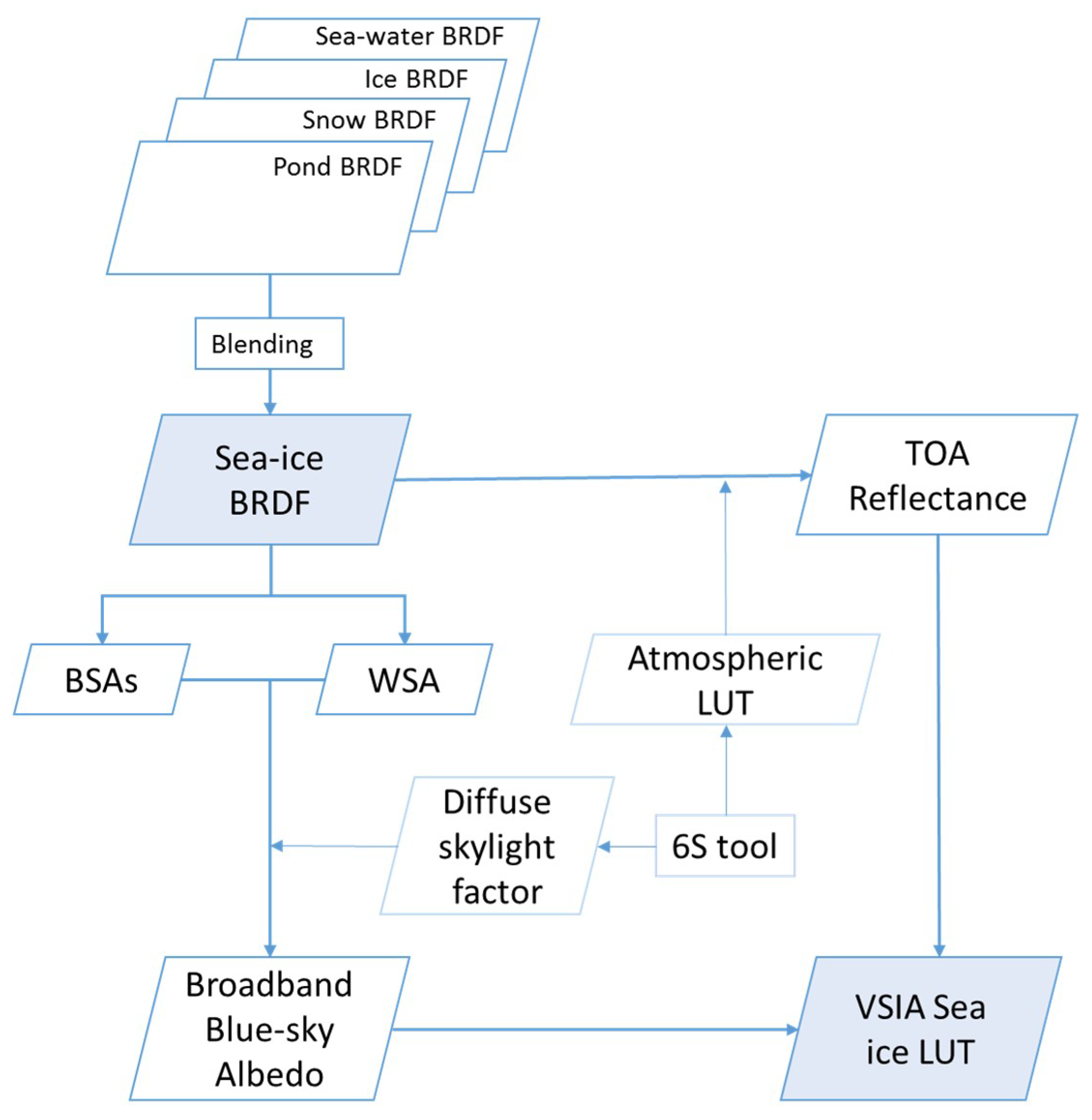
2.2. The BRDF-Based Direct Regression LUT Generation

The broadband instantaneous blue-sky sea-ice albedo is calculated from multispectral top-of-atmosphere (TOA) reflectance using an angular-specific linear regression relationship.

$$\alpha \left({\theta }_s\right)=c_0\left({\theta }_s,{\theta }_v,{\phi }_s\right)+{{\displaystyle \sum }}_b{c}_i\left({\theta }_s,{\theta }_v,{\phi }_s\right){\rho }_i\left({\theta }_s,{\theta }_v,{\phi }_s\right),$$

(1)

where $\alpha \left({\theta }_s\right)$ is the broadband blue-sky albedo; ${\theta }_s$ is the solar zenith angle (SZA); ${\theta }_v$ is the view zenith angle (VZA); and ${\phi }_s$ is the relative azimuth angle (RAA). i (1,2,3,4,5,7,8,10,11) represent the nine VIIRS moderate resolution bands used in sea-ice albedo retrieval. ${\rho }_i$ is the TOA reflectance from sensor data records (SDRs). $c_0$ and $c_i$ are the retrieval coefficients; $c_0$ is the constant term. The coefficients are stored in a pre-defined look up table (LUT) for evenly spaced angular bins in SZA, VZA, and RAA.

The pre-defined LUT trained from the representative dataset renders the algorithm highly efficient and accurate. The algorithm will get the coefficients for an actual $\left({\theta }_s,{\theta }_v,{\phi }_s\right)$ combination through linear interpolation in the surrounding angular bin, which runs fast in operational practices and avoids the discontinuity in neighboring albedo values. The LUT configuration covers SZA from 0° to 80° with an increment of 2°, VZA from 0° to 64° with an increment of 2°, and RAA from 0° to 180° with an increment of 5°.

Figure 1 shows the data flow used to generate the VSIA LUT. The BRDF database is the basis for deriving TOA reflectance and broadband albedo, respectively. This database can be retrieved from satellite data for land surface pixels but has to be simulated from physical models for sea-ice pixels due to the lack of clear and low-SZA satellite observations in polar regions. A satellite pixel in the sea-ice zone was simplified as a combination of snow, ice, pond, and seawater [23]. The sea-ice BRDF can be regarded as a linear composition of the component BRDFs. The contributions of some distributed surface impurities containing dust and soot are expressed in the snow/ice BRDF model [23,26]. The BRDFs of the snow/ice component are simulated using the asymptotic radiative transfer (ART) model, with the input of inherent optical properties (IOPs) calculated from a variety of snow/ice physical parameters [26]. For ocean water, each BRDF is a linear combination of its three components (sun glint, whitecaps, and water-leaving reflectance from just beneath the air-water interface) [27]. The pond BRDF simulation in VSIA LUT deploys the analytical model proposed by Zege et al. [28] with the optical characteristic values referred to by Morassutti and LeDrew [29].

Sea-ice BRDF is considered as the linear mixing of these components’ BRDFs. The fractions of different components in sea-ice pixels vary through time, thus the inherent heterogeneity of sea-ice BRDF should be considered in the simulation process. The Monte Carlo simulation method is used to generate samples of fractions in assembling the sea-ice BRDF for efficiency. The fraction of the first three components is determined by a uniform random number within 0~1. The fractions of the four components used sum to 1 in each BRDF item.

We generated a sea-ice BRDF dataset consisting of 120,000 simulated sea-ice BRDF items. The next key step is to generate the surface albedos. For each sea-ice BRDF item, the surface broadband albedo, including the black-sky albedos (BSAs) and white-sky albedo (WSA), are derived through an angular integration and narrowband-to-broadband conversion. Another method to achieve the sea-ice albedos is by aggregating the BSAs and WSA of each component using the simulated fractions. Its convenience embodies in the direct acquisition of snow/ice/seawater albedo from their BRDF models. The results of the two methods are consistent. The second one was used in our calculation.

The direct estimation algorithm was to directly infer surface albedo from TOA reflectance. Another key step is to simulate the TOA reflectance and diffuse skylight factor in each angular bin from sea-ice BRDF through atmospheric simulation using the 6S (Second Simulation of the Satellite Signal in the Solar Spectrum) tool. To eliminate the uncertainty resulting from atmospheric effects, multiple possible atmospheric conditions have been considered in the training data setup. Sea ice is mainly distributed in the Arctic, Southern Ocean, and Antarctic. The possible atmospheric influence in these regions can be represented in 6S using three predefined atmospheric models including sub-Arctic winter (SAW), mid-latitude winter (MLW), and sub-Arctic summer (SAS), while the typical aerosol types can be described using rural and maritime [30]. In practice, the atmospheric parameters are pre-calculated and stored in an atmospheric LUT. We transferred the surface reflectance spectra under each atmospheric condition type, which is the combination of an aerosol model and an atmospheric model. Then the number of simulated TOA spectra is much expanded than that of the surface BRDF spectra.

For the convenience of users, our retrieval object parameter was set as blue-sky albedo, which is defined as the ratio of up-welling radiation fluxes to down-welling radiation fluxes in a given wavelength range and is comparable with the in situ albedo observations. The blue-sky albedo is estimated using a linear relationship of black-sky albedo (directional-hemispherical surface reflectance) and the white-sky albedo (bi-hemispherical surface reflectance). The diffuse skylight factor has been recorded in the atmospheric simulation and is used as the regulatory factor in combining the BSA and WSA into blue-sky albedo [31] as the regulatory factor (2).

$${\alpha }_{blue-sky}=\left(1-\beta \right){\alpha }_{black-sky}+\beta {\alpha }_{white-sky},$$

(2)

It is assumed that the BRDF dataset is representative to all possible sea-ice pixels in the polar region. Based on the calculation results above, we built linear relationships between TOA reflectance and surface blue-sky broadband albedo for different solar/viewing angular bins using a least squares method. The assumption is that the regression relationship in each angular bin is applicable to various sea-ice surface types with a minimum overall square error over the BRDF database. The regressed coefficients form the sea-ice albedo LUT.

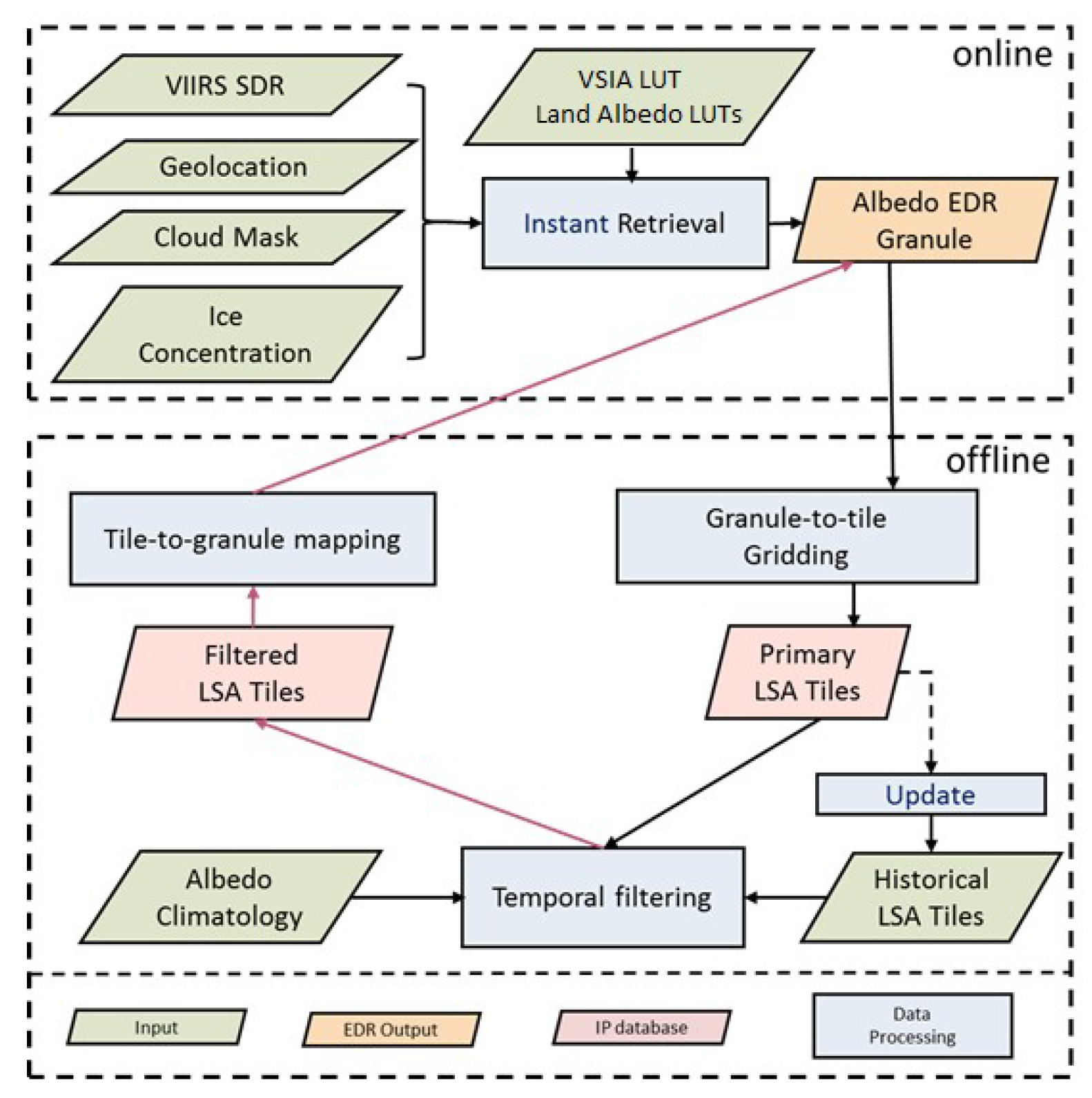
2.3. The Operational VSIA Algorithm

The NDE albedo process consists of two components, as shown in Figure 2. The granule albedo, i.e., the published VIIRS albedo product, is computed online from a combination of the directly estimated albedo and a historical temporally filtered gap-free albedo; the historical albedo is computed offline from the granule albedo of previous days.

The instant retrieval of sea-ice albedo is calculated online from VIIRS TOA reflectance stored in the sensor data record (SDR), with latitude/longitude, solar zenith/azimuth angle, and view zenith/azimuth angle that are stored in a geolocation file. VIIRS NDE cloud mask EDR is used to remove the cloud contaminated pixels. The algorithm also needs the VIIRS Ice Concentration intermediate product (IP) [32] to distinguish the ocean pixels covered by ice.

Instantly-retrieved albedo values are only available for clear-sky pixels which results in gaps in the online generated albedo due to cloud contamination. Therefore, an offline process was designed to provide noise-eliminated albedo for online gap-filling. The offline branch deploys a temporal filtering algorithm [33], which deduces the albedo from a time series of instant retrievals (including the previous 8 day retrieval plus the current day) based on maximum likelihood estimation. Albedo climatology acts as a critical static input to provide statistics about inter-annual trends and variation of albedo for weight calculation and backup value estimation.

To solve the geometric registration problem between multi-day historical albedo images, temporal filtering is conducted on a fixed grid of sinusoidal projection. The global grid is evenly divided into 72 (horizontal) by 72 (vertical) tiles. After online instant retrieval, the albedo granules will go through a forward granule-to-tile transformation prior to offline filtering and a backward tile-to-granule transformation subsequently. The online albedo after gap-filling with the filtered albedo can provide continuous and reliable sea-ice albedo for users.

3. Validation of VSIA Using Ground Measurements

3.1. Ground Measurement Dataset

In situ albedo observation of sea ice is expected to verify the algorithm. However, this type of measurement is rare and its match-up with VIIRS observations is more so. Therefore, we firstly used Programme for Monitoring of the Greenland Ice Sheet (PROMICE) and Greenland Climate Network (GC-NET) measurements as substitutes. Greenland is the world’s second-largest ice mass. Its ice sheet has existed for more than 2.4 million years and covers more than 80% of the island area. Considering the comparability of samples from different seasons, the match-ups around local solar noon (13:30~15:30 UTC time) were used for the comparison. Only the clear-sky observations were retained. The term “clear-sky” is used to distinguish a sky without cloud influence. The cloud effect on the radiation budget, referred to as ‘cloud forcing’, is one of the largest uncertainties in radiative transfer models. It is acceptable to screen out the cloudy-sky days before the comparison.

We also compared the VSIA with some in situ datasets from existing studies. Although the sample size is limited and the measurement footprint is not enough to catch the spatial heterogeneities within the satellite pixel, the comparison would embody the performance of VSIA in actual sea-ice surfaces.

3.1.1. PROMICE Measurements

PROMICE AWS (automatic weather station) is distributed in the ablation zone of Greenland. The surface types viewed are a mixture of snow patches, ice with time-varying physical parameters, and surface ponds, especially during the summer melt season [31,34,35,36,37], which may optically resemble sea-ice surfaces under certain conditions. Therefore, the data was used as a substitute for sea-ice albedo measurements.

The newly-developed PROMICE sites provide high-quality measurements due to their continuous maintenance. The PROMICE automatic weather station (AWS) network currently consists of eight regions each with a minimum of two stations at a variety of elevations on the Greenland ice sheet (the lower one is labeled '_L' and the upper one '_U'). Most stations are located in the ablation area and are thus transitioning from snow-covered to bare ice surfaces through the melt season. Our comparison was applied to 18 PROMICE sites, as shown in

Table 1. The information of the Programme for Monitoring of the Greenland Ice Sheet (PROMICE) stations.

Site Name	Lat (N, deg)	Lon (W, deg)	Elevation (m)	Site Name	Lat (N, deg)	Lon (W, deg)	Elevation (m)
KPC_U	79.8347	25.1662	870	NUK_U	64.5108	49.2692	1120
SCO_L	72.223	26.8182	460	NUK_N	64.9452	49.885	920
SCO_U	72.3933	27.2333	970	KAN_L	67.0955	49.9513	670
TAS_L	65.6402	38.8987	250	KAN_M	67.067	48.8355	1270
TAS_U	65.6978	38.8668	570	KAN_U	67.0003	47.0253	1840
QAS_L	61.0308	46.8493	280	UPE_L	72.8932	54.2955	220
QAS_U	61.1753	46.8195	900	UPE_U	72.8878	53.5783	940
QAS_A	61.243	46.7328	1000	THU_L	76.3998	68.2665	570
NUK_L	64.4822	49.5358	530	THU_U	76.4197	68.1463	760

, from January 2012 to June 2017. In each month, the VSIA granules during 11:00~13:00 (local time) on the 15th day were compared with the ground observations closest in time.

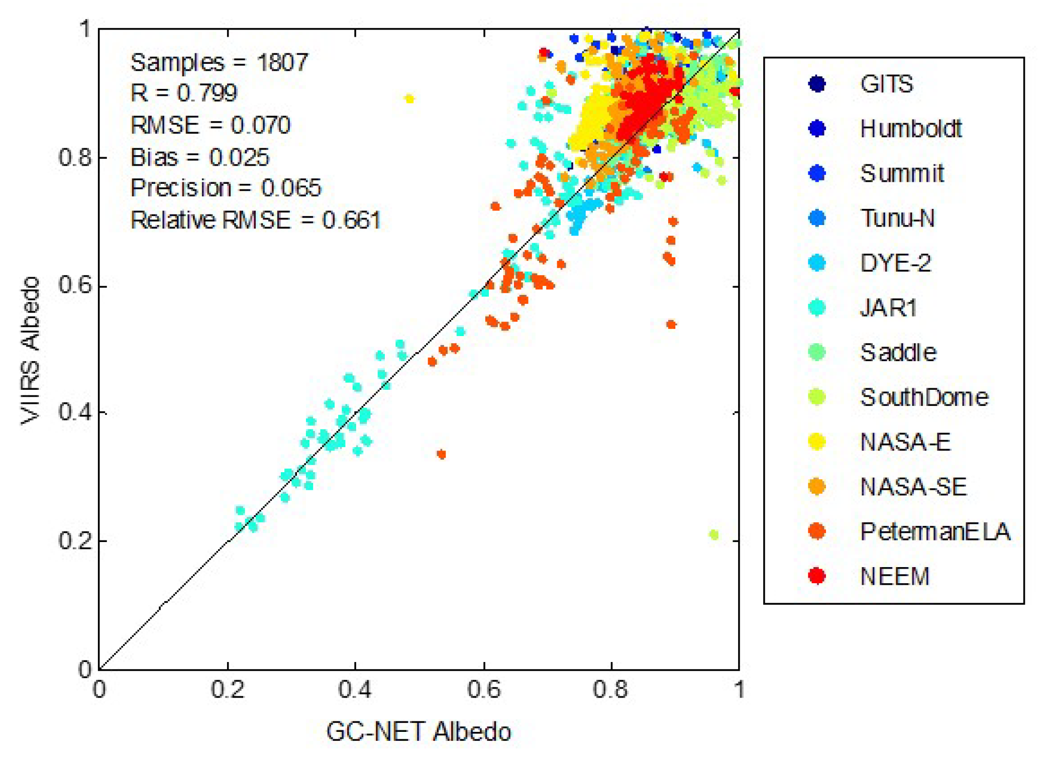
3.1.2. GC-NET Measurements

The GC-NET network has produced a time series of radiation measurements covering the Greenland region since 1995. A detailed description of the GC-NET network and associated instrumentation can be found in Steffen et al. [38]. Although the land cover types of GC-NET sites are not that close to sea ice as PROMICE sites, GC-NET is also a good supplemental data source for VSIA assessment in snow/ice covered regions. We used the available GC-NET data since 2012 for the 13 stations, as shown in

Table 2. The information of the Greenland Climate Network (GC-NET) stations used in this study.

Site Name	Lat (N, deg)	Lon (W, deg)	Elevation (m)	Site Name	Lat (N, deg)	Lon (W, deg)	Elevation (m)
CrawfordPt1	69.8783	−46.9967	1958	Saddle	65.9997	−44.5017	2460
GITS	77.1378	−61.04	1925	SouthDome	63.1489	−44.8172	2850
Humboldt	78.5267	−56.8306	1995	NASA-E	75.0006	−29.9972	2631
Summit	72.5794	−38.5053	3150	NASA-SE	66.475	−42.4986	2400
Tunu-N	78.0164	−33.9833	2113	PetermanELA	80.0831	−58.0728	965
DYE-2	66.4806	−46.2831	2053	NEEM	77.5022	−50.8744	2454
JAR1	69.495	−49.7039	962

.

3.1.3. Field Measurements

We used the data from previous studies [39,40] to evaluate the VSIA performance under various sea-ice conditions in the Arctic, such as the thin first year sea ice and the mixed scenario of sea ice and open water.

Istomina et al. [39] measured the spectral albedo at six ice stations in the central Arctic using ASD FieldSpec Pro 3 during the POLARSTERN cruise ARK-XXVII/3 (IceArc) in 2012. At each station, they obtained surface albedo measurements every 10 m along 200 m transects at 1 m height. A variety of land cover types were observed, including ice, snow, pond, and their mixtures. The spectral albedo was converted to broadband albedo using the solar spectral radiation distribution observed by Hudson et al. [41]. The solar irradiance was corrected to the local measurement time according to the solar zenith angle. All samples at each station were averaged to represent the overall albedo at the pixel scale. The temporally averaged VIIRS albedo during the measuring period was calculated to compare with the average broadband albedo.

Dou et al. [40] measured the spectral snow albedo on the frozen gulf nearby Barrow, Alaska, in 2015. Their measurements were carried out from April to June. The covered land surface types included snow, melting snow, and refrozen snow crust on ice. Spectral albedo was sampled every 5 m along a 100 m line using the ASD FieldSpec Pro 3. Four days of daily mean broadband albedo values were reported, which were used to validate the daily averaged satellite albedo. The dates were 26 April, 18 May, 22 May, and 25 May, respectively.

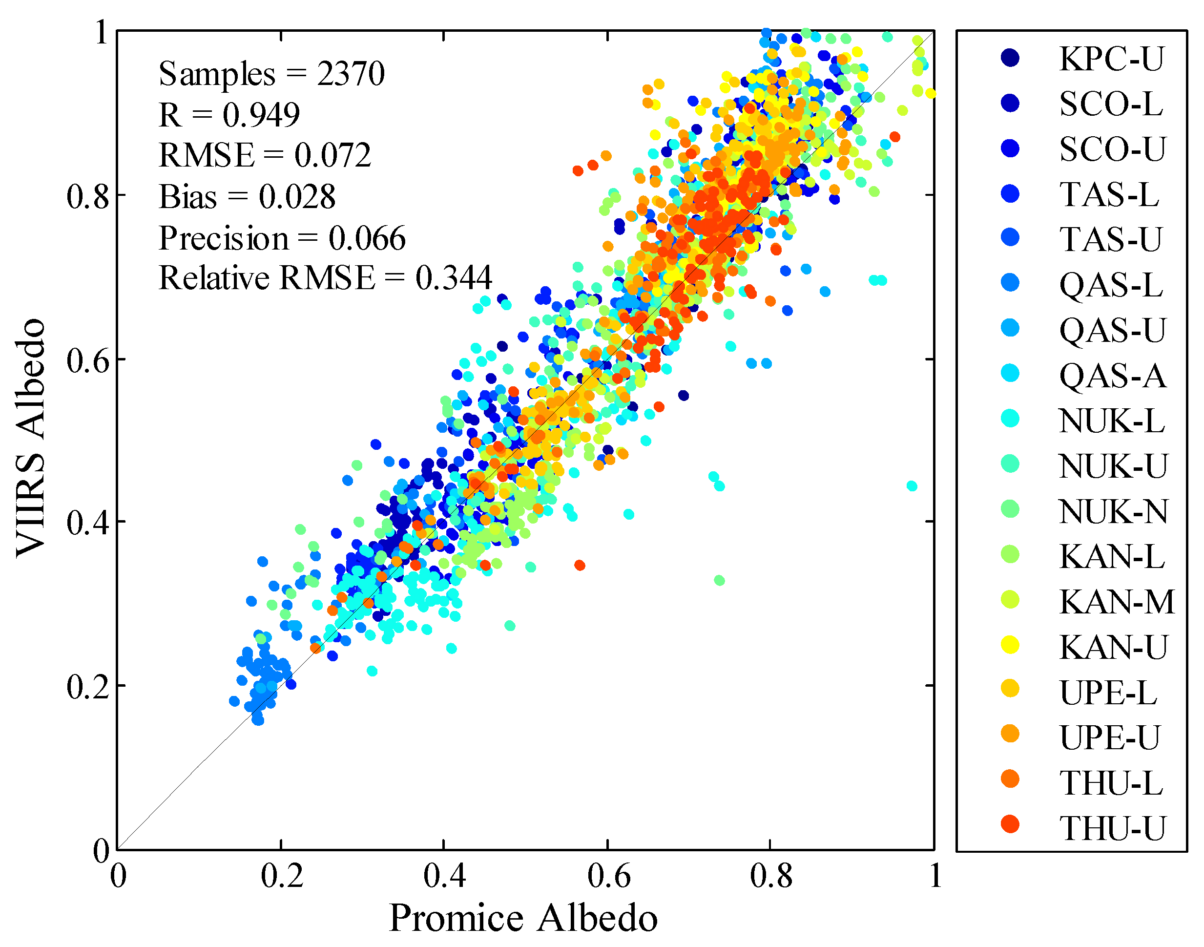
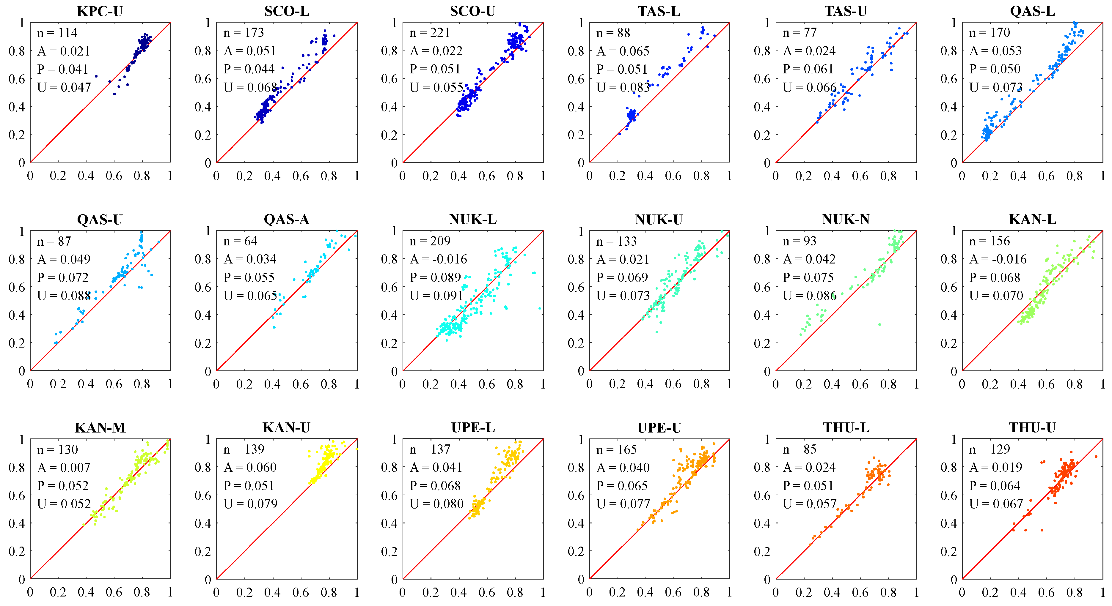
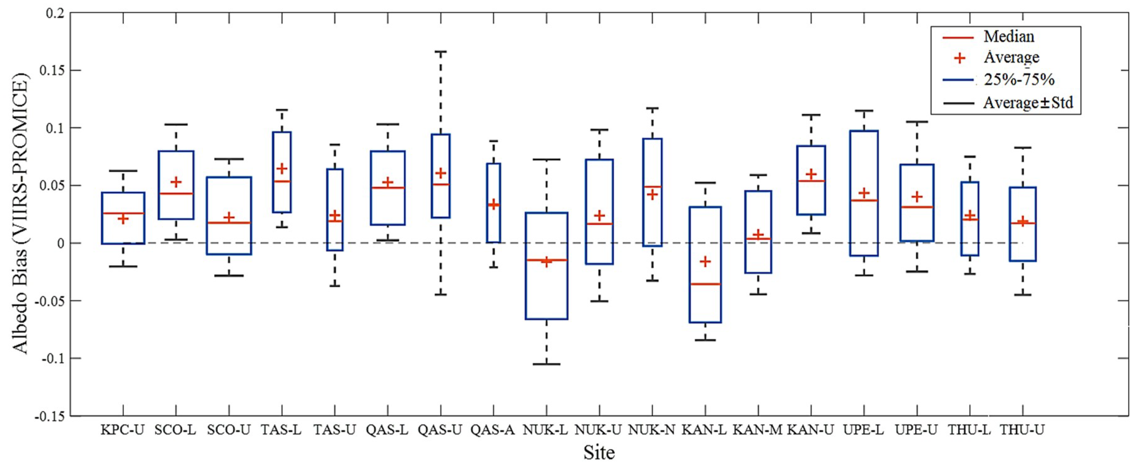
3.2. Comparison between PROMICE and VSIA Match-Ups

The PROMICE-VSIA match-ups span more than five years. The overall scatter plot is illustrated in Figure 3. Comparisons of albedo measurements at each PROMICE station are presented in Figure 4 to show further detail. Additionally, we present the box plot whiskers to show the distribution of the residuals at each station in Figure 5.

Figure 3 demonstrates reasonable agreement between VSIA albedo and the ground reference. Statistical measures that are used to describe these comparisons include the correlation coefficient, the mean difference error (bias), the standard deviation error (precision), and the root mean square error (RMSE) between the two. 1) The correlation coefficient R is 0.947, which indicates an obvious consistency between the two datasets. 2) The bias $\overline{e}$ is 0.028 (about 4.56% relative bias) and the precision $std\left(e\right)$ is 0.066. Here, the bias is calculated as the mean difference between the VSIA and the PROMICE albedo; the precision is calculated as the standard deviation of the difference, showing the spread of the error. The small positive bias shows that VSIA provides slightly higher albedo estimates than the PROMICE measurements. 3) The overall RMSE (root mean square error) is 0.072 and the relative RMSE (Se/Sy) is 0.344. Se/Sy, i.e., the ratio of RMSE to the unbiased standard deviation of the in situ albedo. The goodness of fit indicates a high accuracy of the albedo retrievals using the rule of thumb that Se/Sy < 0.5 represents good accuracy.

The albedo values span from 0.2 to 1, which means that the dataset might contain observations of ice/snow, water ponds, bare ground, or a mixture of those, indicating the extensive representativeness of the sample. The goodness of fit is comparable with the previous validation result of MOD10A1, a regional albedo product over Greenland, Iceland and the Canadian Arctic Region, by Ryan et al. [37]. After post-processing including de-noising and calibration of the MOD10A1 albedo (Collection 6), its RMSE with PROMICE ranges from 0.017~0.1 over three KAN sites between 2009 and 2016. In summary, the validation of VSIA shortwave albedo against ground measurements showed promise at the PROMICE sites.

At many sites, an overestimation of VSIA albedo is exhibited in high albedo regions, as shown in Figure 4 and Figure 5, such as SCO-L, TAS-L, QAS-L, QAS-U, KAN-U. These sites contain both the south (TAS, QAS, KAN) and north (SCO) stations, covering a broad latitude range. In combination with the box plot of error between VSIA and in situ albedo, as shown in Figure 5, it is shown that most stations overestimate albedo by about 0.05. An exception of underestimation happens at NUK_L and KAN_L as a large fraction of their observations lie in the lower value regions. These two sites are located in the southern Greenland ice sheet at 500~700 m elevation, having more obvious characteristics of the ablation zone. The land cover type transitions from dry snow to melting snow to glacier ice at melting season.

The boxplot also suggests that 14 of the 19 stations contain the zero bias within μ ± σ data range, demonstrating that the differences between the VSIA albedo and the PROMICE station data are in general indistinguishable from zero. The sites with a larger spread of albedo error suffer from the smaller sample size, making it difficult to reach solid conclusions on the product’s performance at these sites. It is also illustrated that the mean values of most stations are larger than the median value, suggesting the distribution of residuals are skewed and the higher albedo points are dominant.

According to the site-specific validation results, VSIA albedo demonstrates strong sensitivity to in situ surface albedo fluctuation and anomaly. (1) VSIA shows lower albedo value at NUK_L and KAN_L, which are the lower stations on the southwest Greenland coast, while demonstrating higher albedo values at other sites. NUK and KAN are two typical regions reported of albedo anomaly due to darker-than-average ice caused by a stronger warming trend, higher melt, and less winter accumulation [42,43,44]. Their bias derives from many factors. First, it is mainly attributable to the scale difference. The in situ measurements have a much smaller footprint than the satellite retrievals. The higher impurity concentration around these two sites leads to stronger surface spatial variability, especially in melt seasons [45,46]. Second, the bias might be ascribed to the absence of some dark zone constituents in the VSIA algorithm, including algae, crevassing, supraglacial water, and cryoconite distributed in the Greenland ice sheet [45]. The third attribute is the topography’s effect. Some of the PROMICE stations are located on slightly sloping terrain. Sloping terrain alters the incident radiation composition and solar/view zenith angles, which would introduce wavelength dependent uncertainties in satellite albedo retrievals [47]. (2) For most regions, the upper station has lower bias than the lower station, such as SCO_U and SCO_L, TAS_U and TAS_L, UPE_U and UPE_L, and THU_U and THU_L. Lower sites have earlier melt onset and suffer from severe fluctuations. The scale difference between satellite retrieval and ground measurements is amplified. (3) The largest RMSE appears at the north tip site and the smallest RMSE corresponds to the south tip site. RMSE shows a slightly negative relationship with the latitude belt since southern Greenland has a much warmer summer and earlier melt than the northern regions.

3.3. Residuals Analysis

The main purpose of validation is to evaluate and improve the model accuracy. The residual between VSIA and PROMICE albedo measurements were analyzed with the related factors. First, the seasonal change of albedo values and the bias trend were observed. Second, the annual trend of the most important environmental factor for snow/ice albedo (SZA) was analyzed with the albedo time series and residuals. Finally, the influence of another important factor for in situ validation—ground heterogeneity—was also considered.

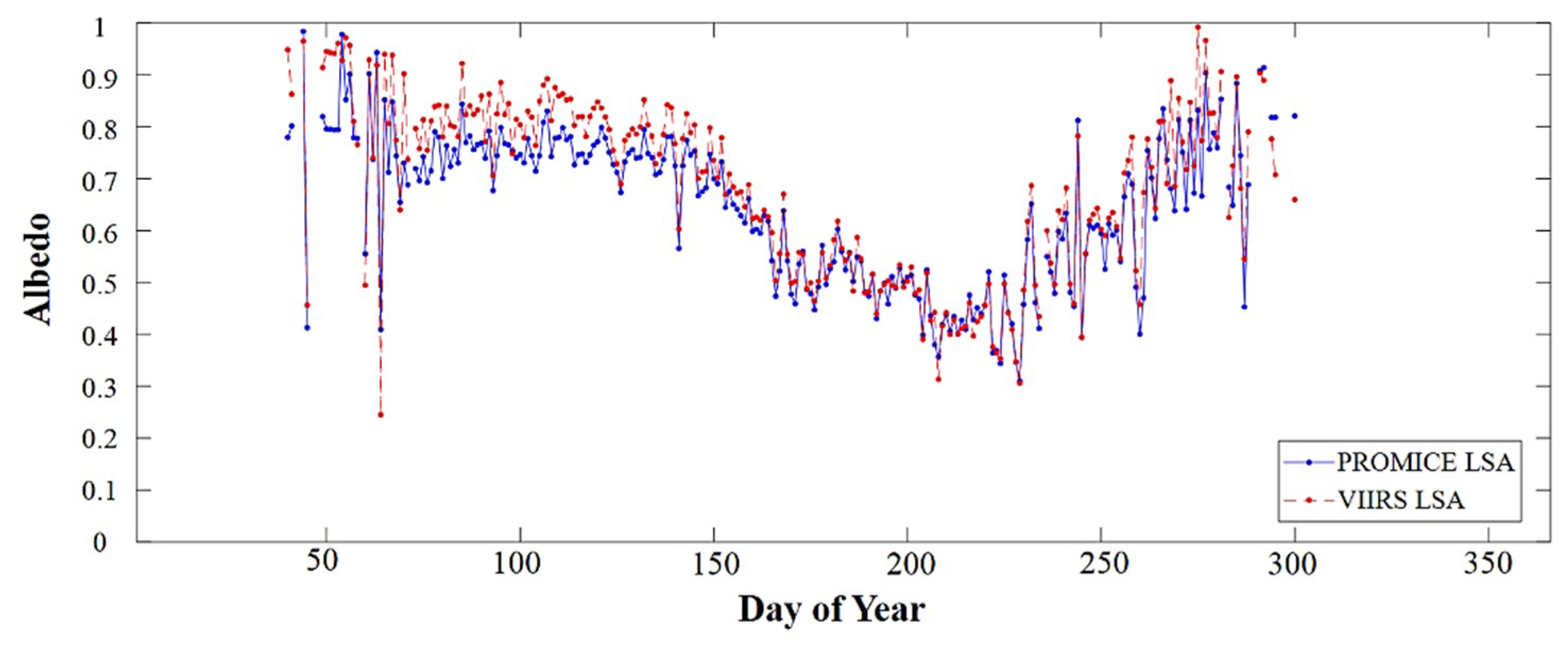
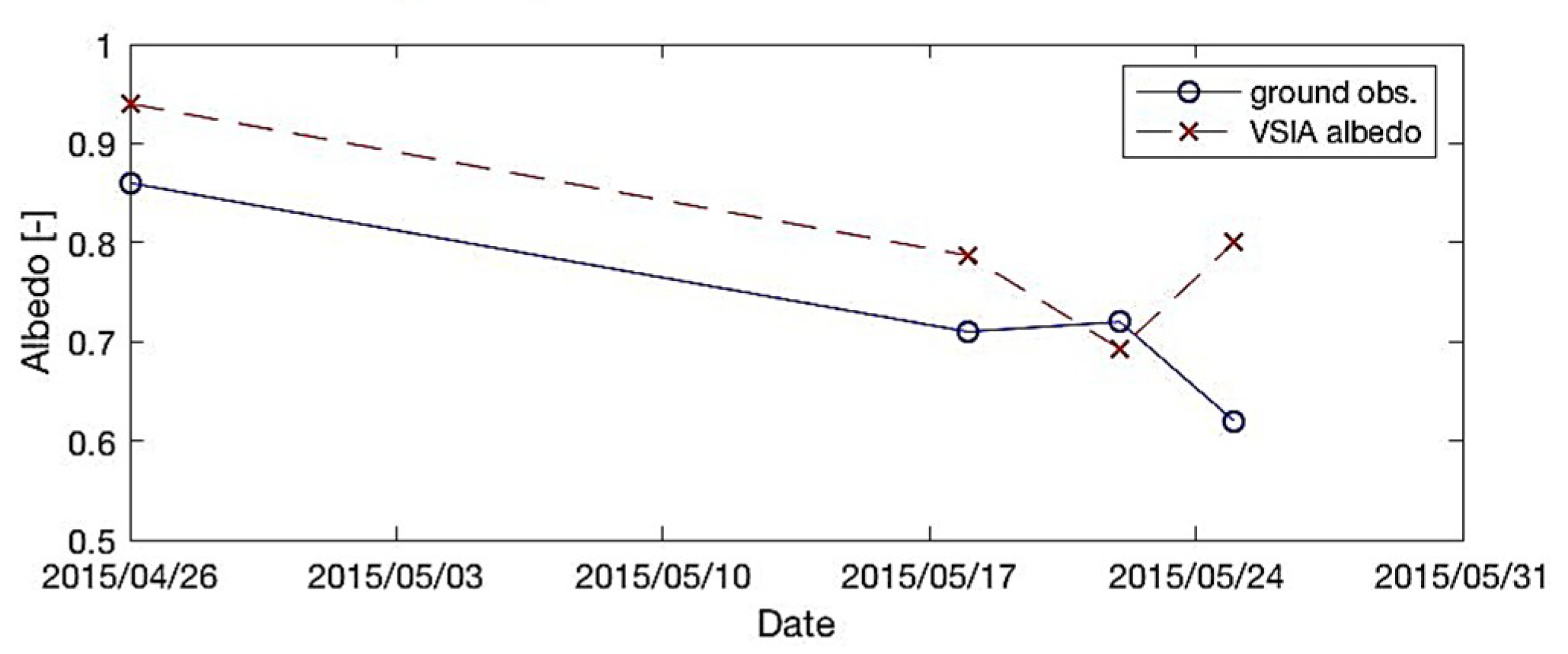
3.3.1. Temporal Continuity and Variability of Albedo

Figure 6 demonstrates the annual variation curves of the VSIA and PROMICE albedo. It is shown that the VSIA albedo and PROMICE albedo time series agree well with a cross-correlation coefficient of 0.9554, illustrating a significantly strong correlation.

The surface albedo of the ablation area changes with the coverage fractions of snow, bare ice, and dark impurity-rich surfaces. Accordingly, the corresponding difference fluctuates at different seasons along with the ice/snow melting and accumulating cycle. Albedo value fluctuates intensely in winter responding to the snow events. Snowfall will cause a large albedo value and its melting will decrease the surface albedo. When summer approaches, the ice melts first and the pond fraction increases, causing the albedo to drop to its minimum value at the end of July. Then, the freezing of ponds increases the albedo again.

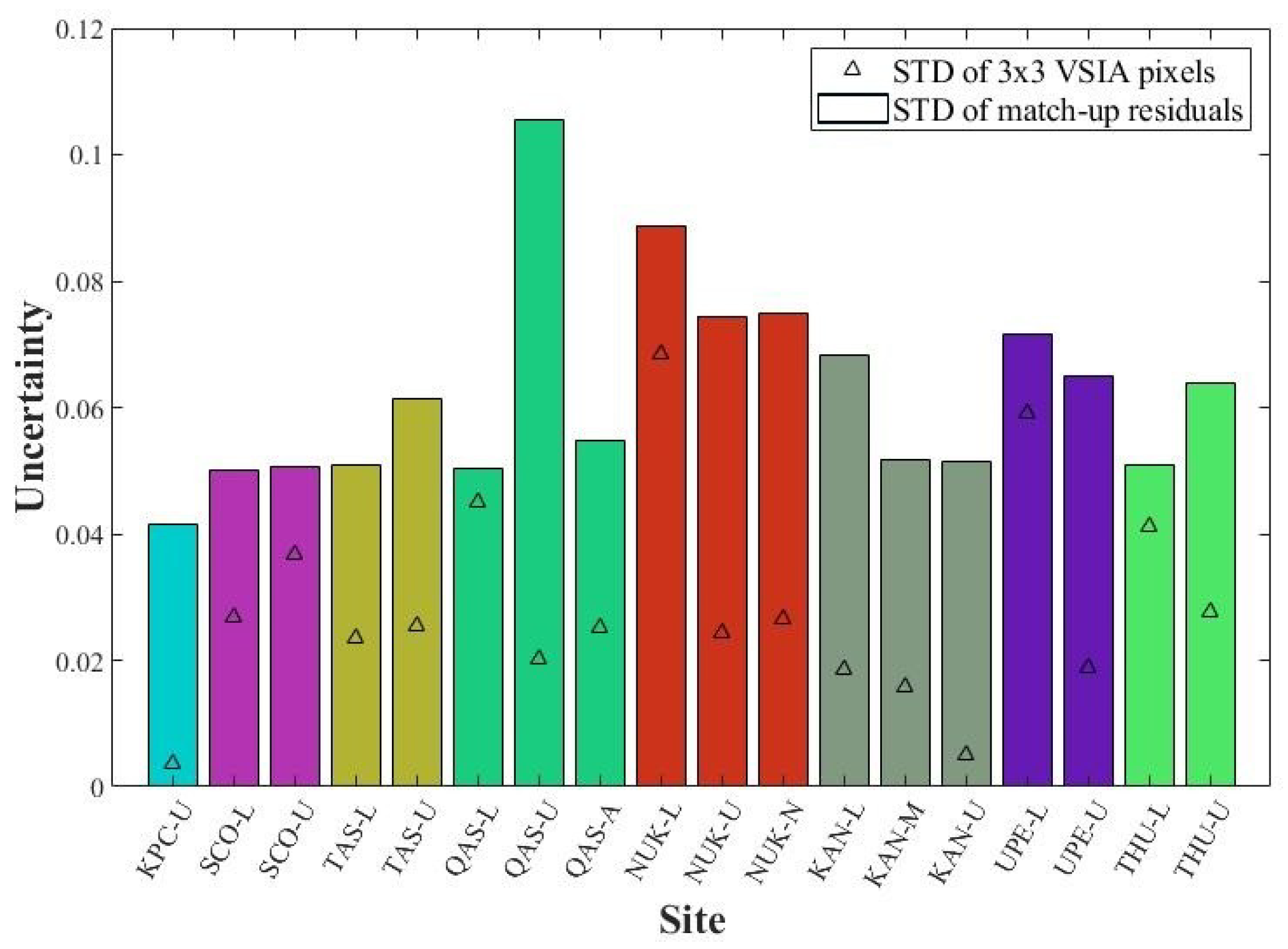
3.3.2. Influence of Heterogeneity

Considering the complex land cover types and the topography variation that surrounds many of the PROMICE stations, the standard error of albedo in the 3 × 3 neighboring pixels was analyzed to assess the effect of the local heterogeneity, as shown in Figure 7.

Here, a range of 3 × 3 VIIRS neighboring pixels is chosen to assess the spatial heterogeneity at satellite level considering the maximum geolocation error of VIIRS M-band SDR data [48]. Figure 7 illustrates the mean standard deviation of albedo within 3 × 3 neighboring pixels and the standard deviation of the residuals between VSIA and PROMICE albedo at the center pixel. It is shown that the albedo heterogeneity is correlated with the spread of the match-up residuals within the same region. This inference is not applicable for cross-region comparison due to the interference from the different albedo magnitudes and distinct land cover compositions. Exceptions include stations in the QAS region and the THU region, which may be due to the limitation of the albedo map used in our analysis. A higher resolution albedo map is preferred to assess the around-site heterogeneity.

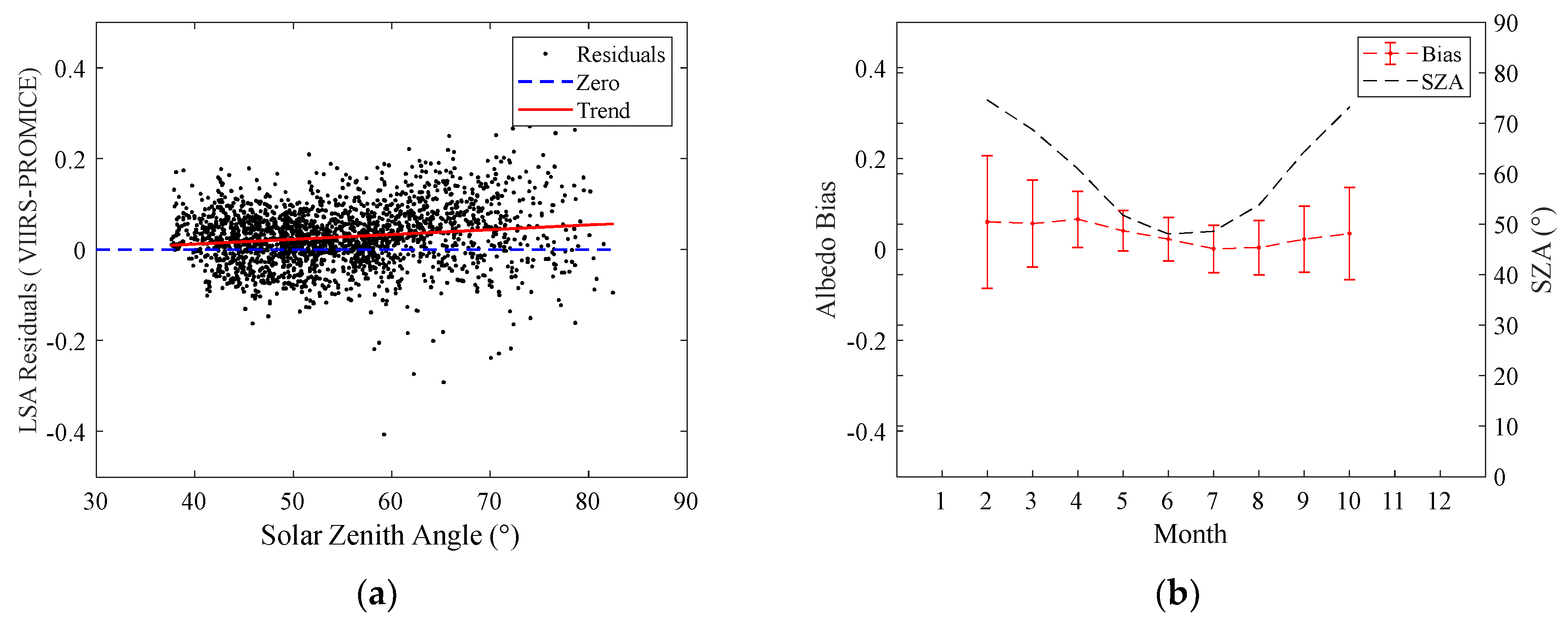
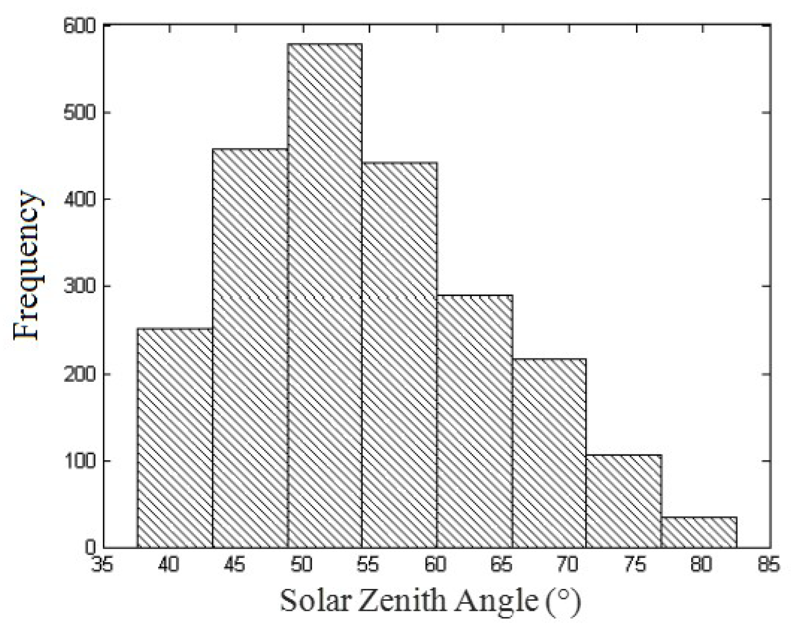
3.3.3. Influence of Solar Zenith Angle

Due to the high latitude of the Greenland region, the solar zenith angle corresponding to the observations are distributed from 38° to 82° and peak around 50°~55°, as shown in Figure 8.

The bias between the VIIRS albedo and PROMICE observations exhibit a slight increasing trend with SZA, as shown in Figure 9. SZA determines the fraction of the direct incident radiation and the directional-hemispherical albedo component. It influences the diurnal/seasonal variation of surface albedo. For clear-sky snow/ice albedo, the photons interact with the snow grains over a longer path at larger SZAs, which will result in more interaction with snow surface and higher absorption [49]. At larger SZAs, the retrieval uncertainty of VSIA increases due to the strong anisotropy of the snow/ice surface. Meanwhile, the measurement error of the cosine instrument increases at larger SZAs. They together lead to the larger standard albedo error at larger SZAs.

It is known that SZA at solar noon time is larger in winter than summer. Therefore, a larger bias would be observed in winter.

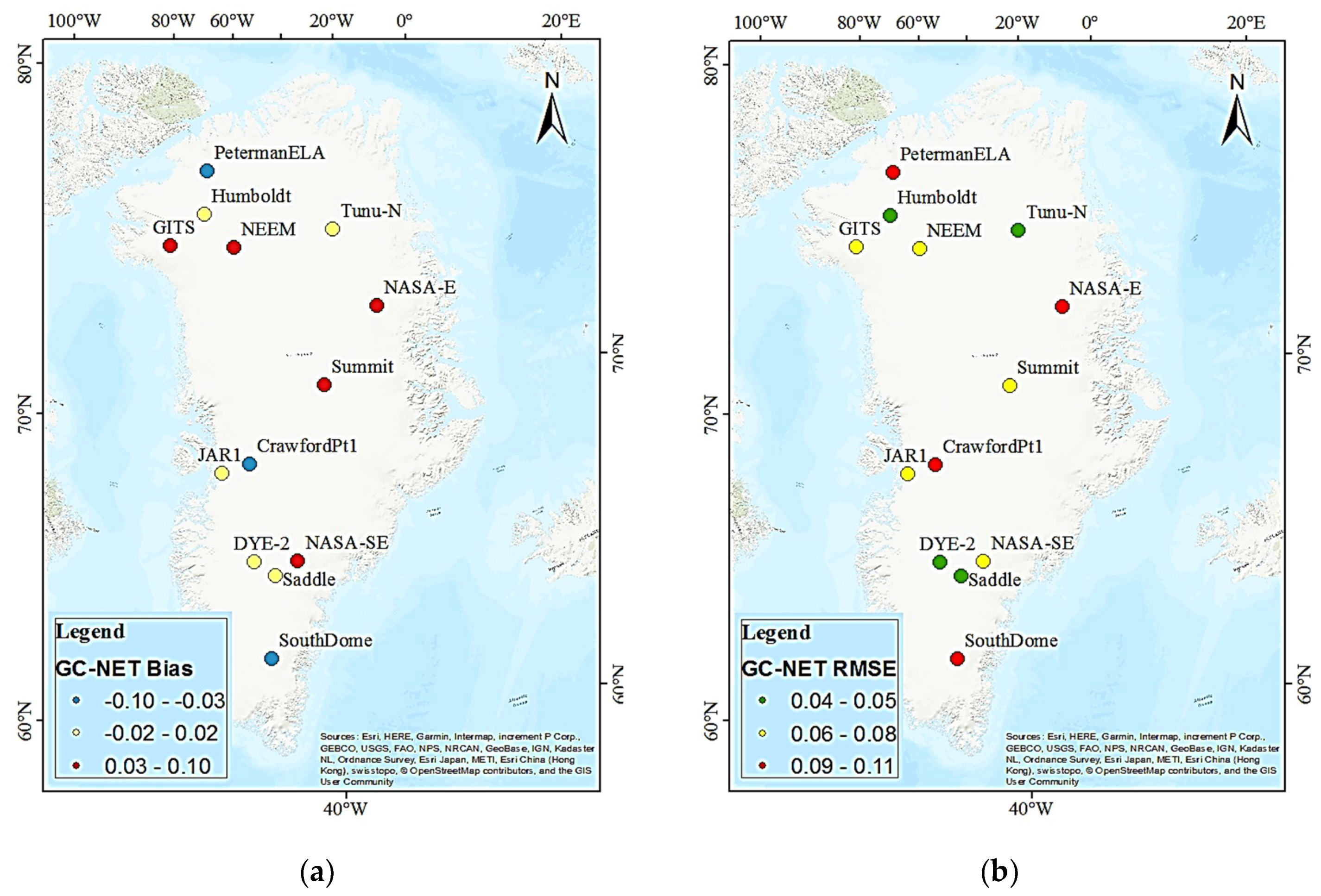
3.4. Validation Using GC-NET Match-Ups

The validation results over GC-NET sites showed a similar estimation accuracy of VSIA albedo to that over PROMICE sites. The absolute value of overall accuracy is 0.025 with a precision of 0.065, as shown in Figure 10. This is acceptable as the precision of GC-NET observations is around 0.05 [38]. The overall root mean square error is 0.07, while the relative RMSE of 0.661 is showing 66% of the unexplained variance. Similar to the PROMICE validation result, VSIA and the GC-NET measured albedo is generally consistent with better agreement at the ablation zone of lower albedo. Note that some outliers appear at the PetermanELA site, showing larger observations from GC-NET than VIIRS retrievals, that are caused by surface heterogeneity and geometric match uncertainty.

The goodness of fit at different sites displays some spatial patterns, as shown in Figure 11. This implies that the validation results are influenced by the elevation, latitude, and land cover types of different sites. The validation results at red-colored sites show that VSIA has an underestimation of albedo compared with GC-NET observations, with a higher RMSE. These sites distribute in the northernmost and southernmost regions and suffer more from surface heterogeneity. At the green-colored sites, VSIA has more accurate estimations and shows lowest bias and RMSE. At the blue-colored sites, VSIA slightly overestimates ground albedo and shows moderate RMSE.

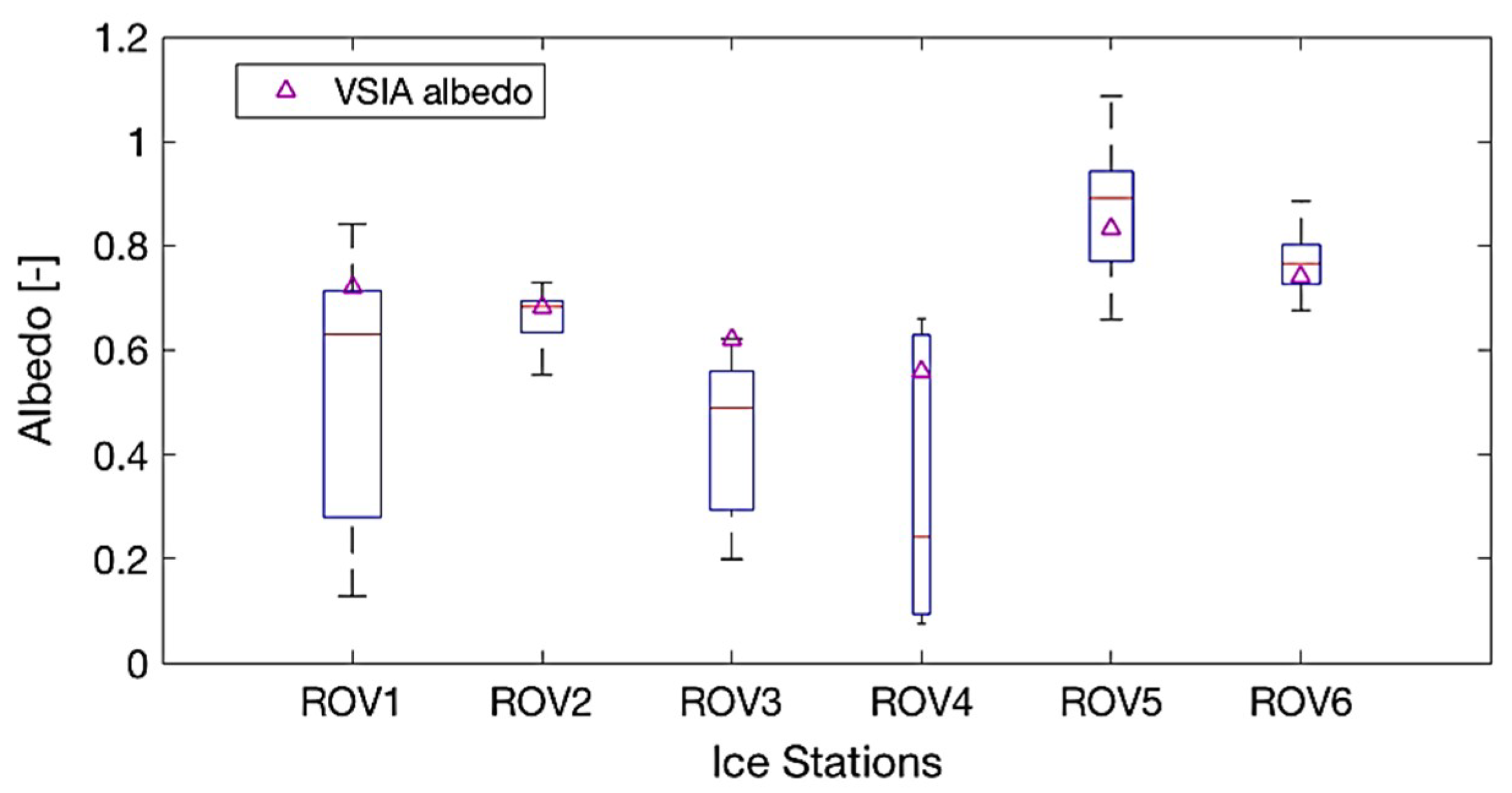
3.5. Evaluation of VSIA Using In Situ Sea-Ice Albedo

Figure 12 shows the comparison between VSIA and Istomina’s measurements [39]. The VSIA values all fell in the range of the ground samples at all the six ice stations. The bias between the two datasets is 0.09. It should be noted that the satellite-derived albedo is instantaneous and averaged spatially; surface measurements are local and averaged temporally. The strong spatial heterogeneity and the albedo variation around the station have introduced large uncertainties to the comparison. Moreover, the in situ measurements were directly averaged without considering the contribution weight of each land cover type due to the lack of auxiliary data. Based on the comparison, we can infer that the VSIA correctly reflects the albedo magnitude of the sea-ice regions covered in the experiment.

The daily mean albedo [40] was collected from one site on different dates. Figure 13 illustrates the time-series plots of VSIA and ground observations. The albedo values generally match with a bias of 0.077. The albedo discrepancy varies along with the sea-ice evolution. (1) The sign of the discrepancy changed at the third match-up because there was a snow event on 20 May so that the spatial distribution of surface albedo changed. (2) The last match-up happens in the sharp snow-melting period. The strong spatial heterogeneity with snow accumulation and melting mainly contributes to the large albedo discrepancy.

4. Discussion

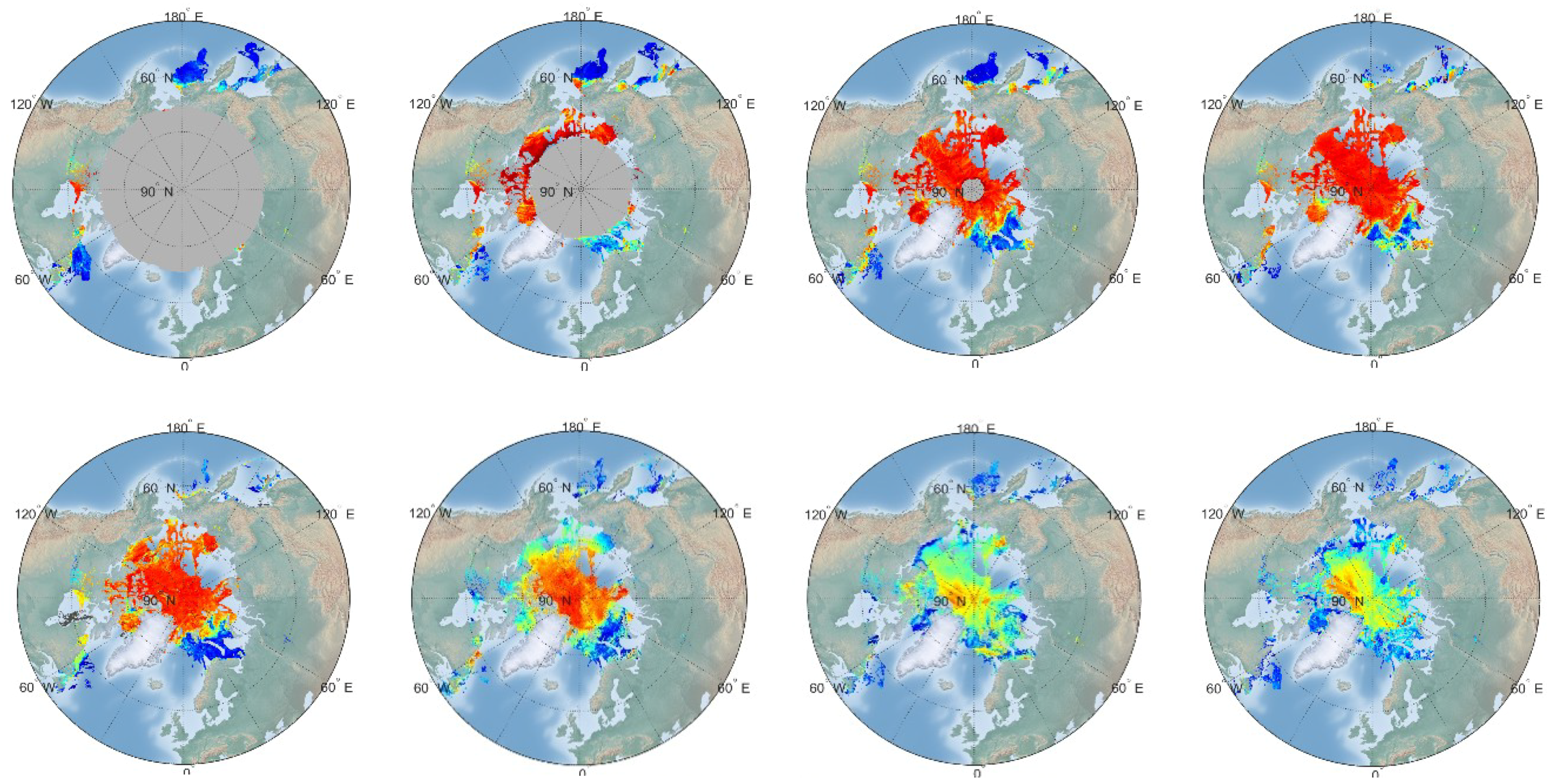
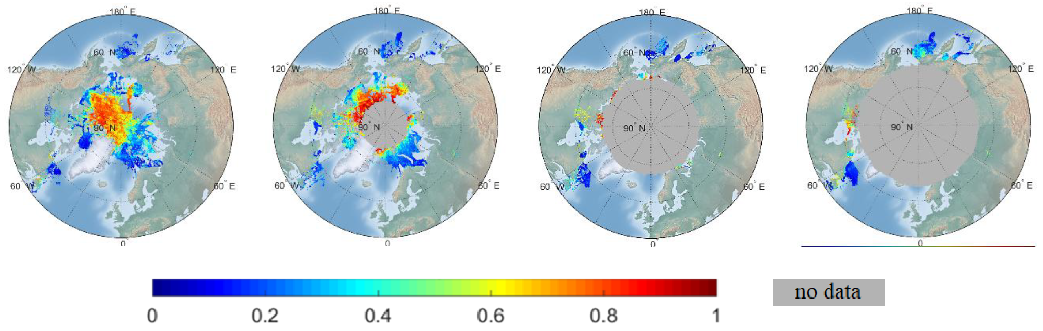
4.1. Northern Hemisphere Albedo from VSIA

VSIA albedo offers a fine-resolution, large-scale albedo data source. Figure 14 shows monthly albedo maps in 2014 for the Arctic region as a sample of the algorithm performance. The dynamic evolution of albedo over time is mainly caused by the melt timing and intensity. The coverage of the retrieved albedo increases from January to April after the winter solstice. Then albedo stays at a high value because of the covered, cold, optically thick snow. As temperature increases from May to August, the snow begins to melt, thereby decreasing the surface albedo. Due to the formation of larger melt ponds, the albedo value decreases rapidly during this period. Once the new seasonal ice begins to freeze from ponds and open water, albedo increases again. From October, the data in the central Arctic is missing during the polar night period.

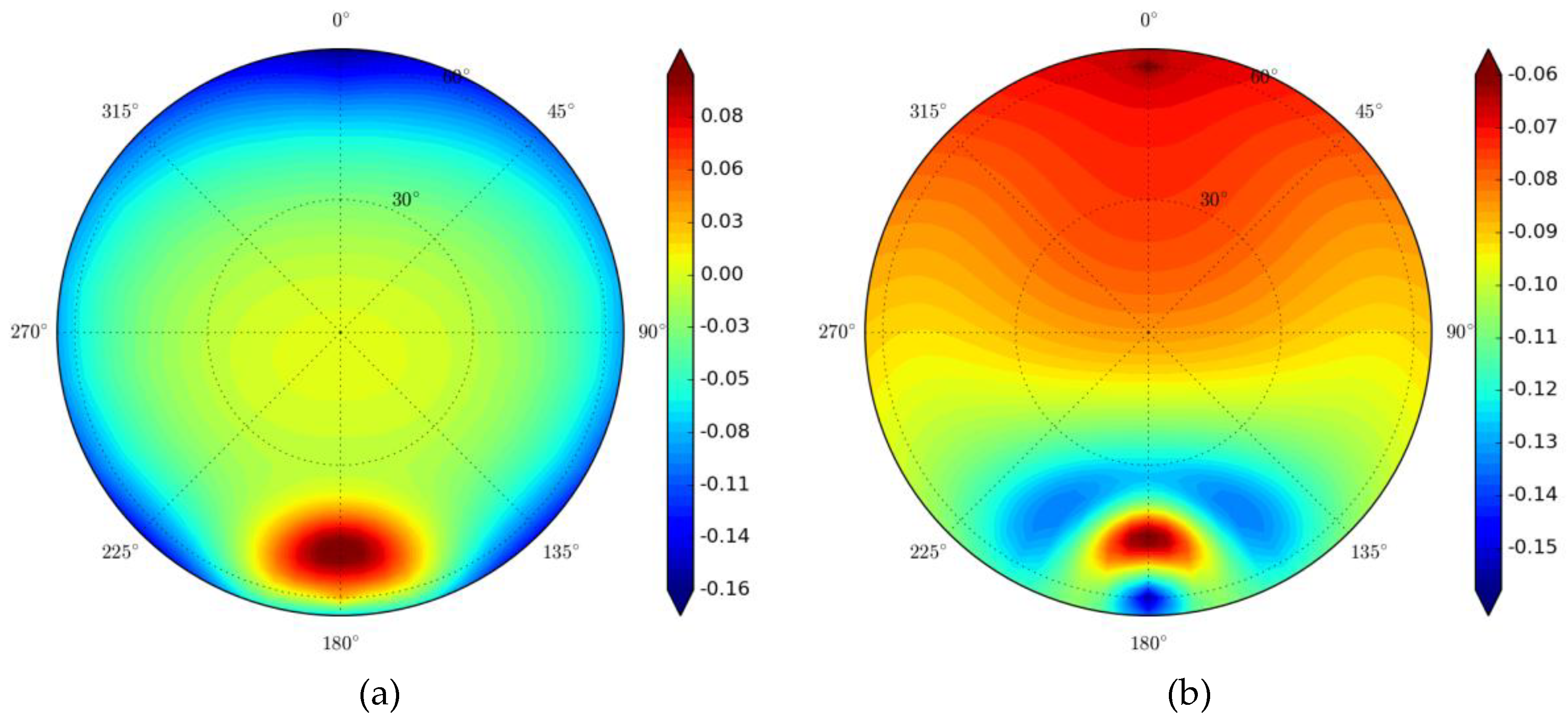
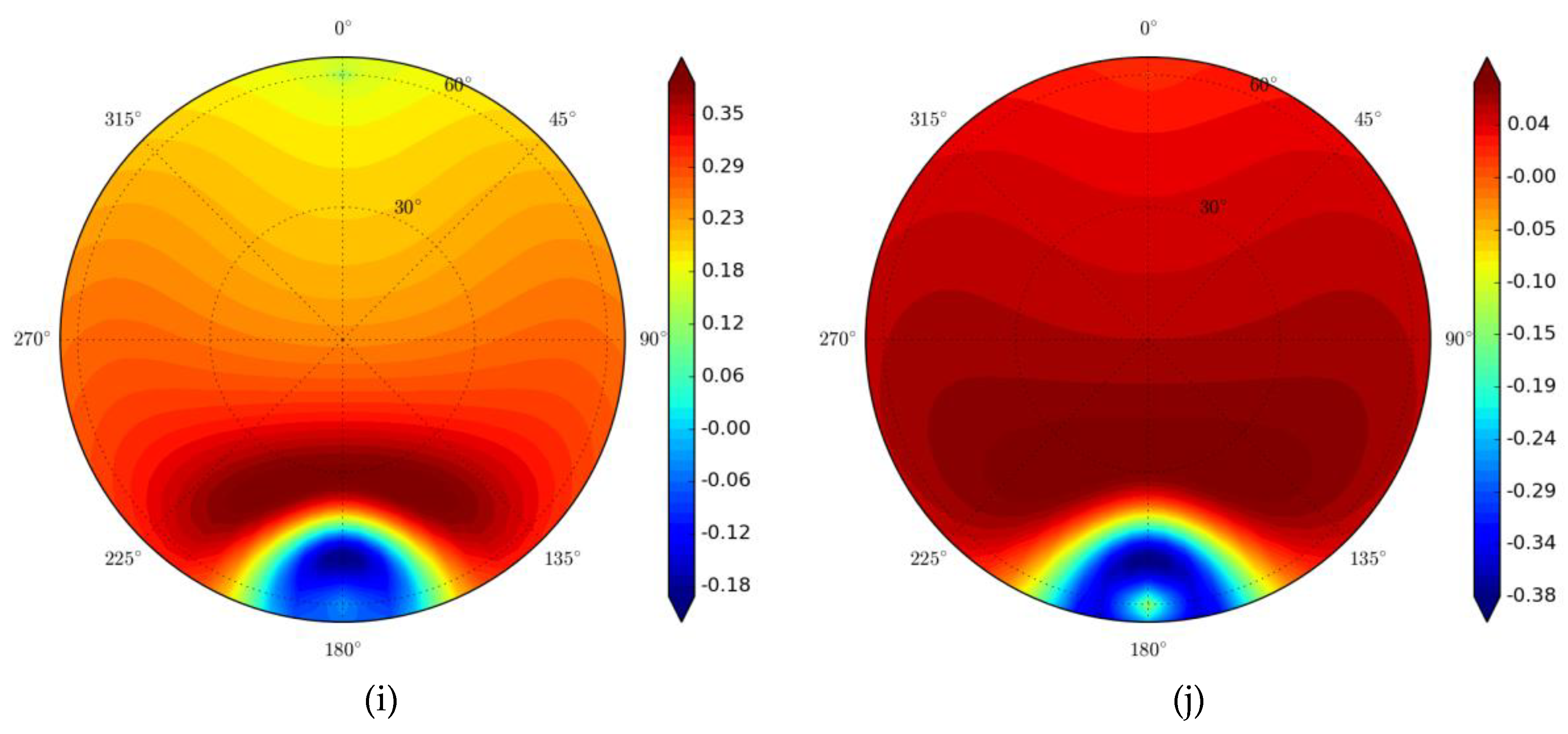
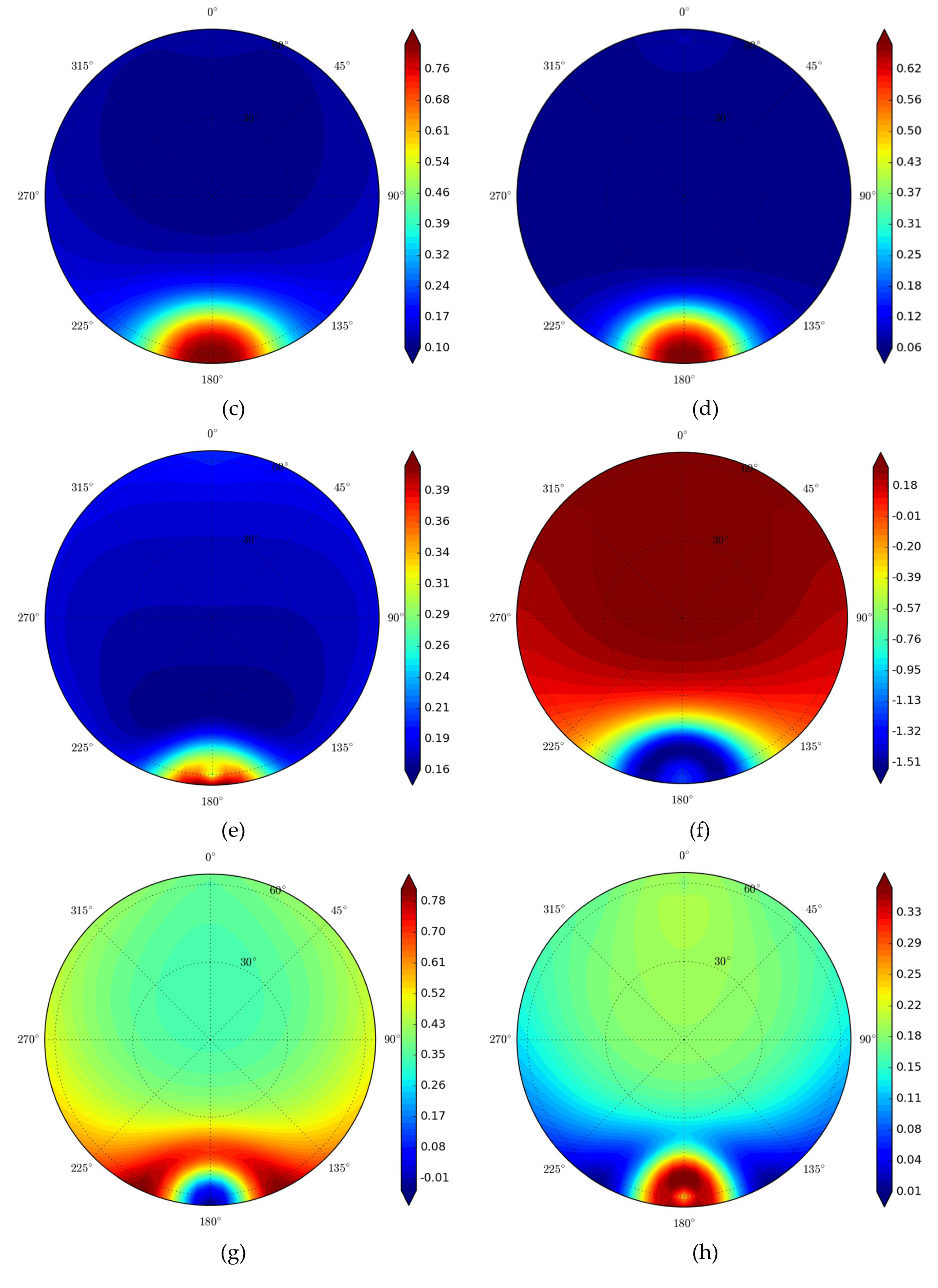
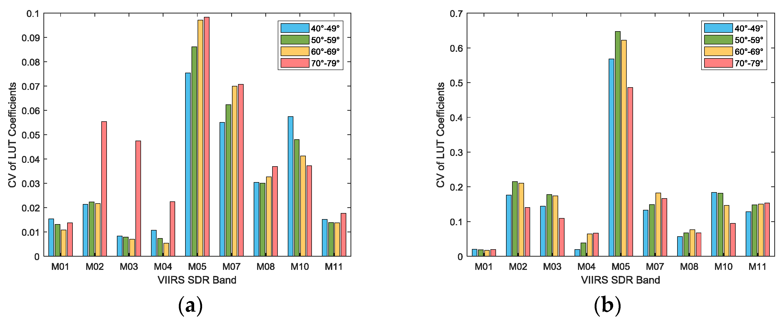
4.2. Analysis of VSIA LUT

The VSIA LUT provides mathematical weights used to convert TOA reflectance to surface broadband albedo, reflecting the energy contribution among different bands at each specific angular bin. Due to the numerical regression process, the coefficients’ magnitudes have lost their direct link to the BRDF directional reflectance intensity, but still reflect some directional variation patterns. For sea-ice covered regions, the SZA is normally larger than 40°, so we picked 60° as an instance to observe the hemispherical variation trend of the coefficients at each SDR band. Figure 15 demonstrates the polar plots of the band coefficients at various VZAs and RAAs with constant SZA. Generally, the polar plots demonstrate the continuity and rationality of VSIA LUT at angular dimensions.

The most apparent feature of all plots is the bright/dark spot in the forward scattering direction, which is formed due to specular reflection over the snow/ice/seawater surface. The specular component in BRDF is in accordance with geometric optics. Its contribution varies with the sea-ice surface physical characteristics and the solar zenith angle. It is shown that the center points of these spots are all around the symmetry point of solar incident direction. The size of the specular reflection spot varies among different bands due to the angular distribution of the spectral reflected flux. For instance, the center wavelengths of M02 and M03 are close, thus their coefficients show similar hemispherical variation patterns.

The phenomenon that the albedo uncertainty increases at larger SZAs shown in Section 3.2.4 is partly due to the increasing spread of LUT coefficients. Here we calculated the coefficient of variation of LUT coefficients at consecutive SZA intervals, as shown in Figure 16. The coefficient of variation measures the relative variability, which is the ratio of the standard deviation to the mean value. The samples cover the whole VZA range. To eliminate the influence of the specular reflectance spot regions, the RAA was divided into two ranges, 0°~150° and 150°~180°, shown separately in Figure 16. The left figure contains a larger portion of RAA values and represents the majority of observations. It shows that the spread of coefficients in the SZA range of 70°~79° is more significant than other ranges at most visible bands. This causes the larger spread of LUT coefficients at larger SZA values. In the forward scattering cases shown in the right figure, the SZA range of 50°~69° corresponds to larger coefficients of variation. But its influence is limited due to the smaller RAA range. The magnitude of bar plots at different bands is related to the spectral sensitivity of albedo to SDR reflectance. The highest value is shown at M05 with a center wavelength of 0.672 μm (light red).

4.3. Limitations in Current Algorithm and Validation

Currently, sea-ice albedo data is going to be produced in the VIIRS albedo environmental data record (EDR). Reliable albedo values were reported through the validation and test in the algorithm readiness review; however, the current VIIRS albedo product over the sea-ice surface still suffers from several issues:

1. Limited validation data on the sea-ice surface

Admittedly, the power of this study is inevitably restricted by the limited sea-ice surface measurements due to rare physical access. The albedo of glacier and sea ice is influenced by the same factors [52], and most of the sea-ice components or their proxies, the ice, snow, and pond, can be found around the Greenland AWS sites, except the sea water surface, which has a very low and relatively constant albedo. Therefore, the long-term monitoring data from the AWS on Greenland has provided substitute reference data for a variety of sea-ice surface conditions, such as the optically thick sea ice with snow cover or melt ponds. It can be seen that the albedo evolution trend over the PROMICE stations, as referred to in the time-series plots in Figure 6, is consistent with the multi-year Arctic sea ice [53].

For seasonal young sea ice, its albedo is typically less than the multiyear sea ice during the melting season and pond evolution [54]. Considering the lack of representativeness of Greenland AWS measured albedo to seasonal sea ice, we also cited some sea-ice albedo measurements as complementary data, which cover the surface conditions such as young sea ice and thin melt ponds. Considering the sample number of the in situ sea ice measurements is limited, further validation attempts are expected to understand the product accuracy, such as cross-comparison with other sea-ice albedo products.

2. Significant validation uncertainty at large SZA

Large SZA affects the accuracy of both VSIA and PROMICE measurements. AWS sensors suffer from the intrinsic cosine response error at large solar zenith angles, which is reported to reach a maximum of 8% at a solar zenith angle of 80° [55]. Even for solar zenith angles less than 75°, we should expect a cosine response error around 5% [56], which can even be amplified by the riming. For VSIA, the ART model for snow/ice BRDF simulation is applicable at high solar zenith angles up to 75° [57,58].

3. Thorough spatial representative investigation is desired

In this study, we did not exclude any match-ups influenced by strong ground heterogeneity since high product performance under all conditions is expected. However, it has been investigated that ground heterogeneity around the sites will amplify the uncertainty in validation at different spatial scales [59]. In this way, further investigation using higher resolution imageries as ancillary data is on schedule.

4. Further investigation on the overestimation reason

The evaluation result shows an overestimation of the VSIA albedo. However, several issues should be kept in mind before drawing this conclusion. First, the ground measurement data does not represent the “true” value considering the big scale gap between the ground point measurement and the satellite pixel retrieval. Second, the measurements from the flux instruments contain certain uncertainty [55], due to the tilting/leveling errors and the cosine-response error of the instruments. Third, the seawater component is absent in this evaluation. According to the current result, the VSIA product performs very well in the low albedo condition; however, the missing seawater component might take some unknown influence into the algorithm performance. To solve this problem, we plan an inter-comparison by introducing other coarser resolution satellite sea-ice albedo products.

5. Influence of sea-ice algae has not been considered

Algae aggregates alter the optical properties including albedo of pond areas [60,61]. The short-lived algal layer growing on the bottom of the ice in springtime resulted in an increasing of the radiance absorption and possible decreasing of surface albedo. This influence was not considered in the theory used for pond simulation in our algorithm, which could be one reason for the overestimation of the VSIA. The improvement of the model to represent the algae optical properties is expected.

6. Some assumptions of the ART model may be violated in the Arctic

The ART model performs well in reproducing the snow/ice reflectance, but still suffers from many problems. First, it is valid for weakly absorbing semi-infinite turbid media [57] so that its validity over the first-year ice still needs further evaluation, since the sample used here is small. Second, the model assumes a flat smooth surface condition. This simplification increases the retrieval uncertainty due to slope and surface roughness [47].

The sea-ice surface roughness also affects the albedo significantly. Increased roughness generally alters the incident and reflected radiation. Its influence on the albedo thus depends on the ratio of diffuse to total incoming radiation. The evaluation of such an effect deserves more extensive work, i.e., considering micro-tomography adjustment in the regression.

5. Conclusions

The surface energy balance of the polar region is mainly dependent upon the surface albedo characteristics. Ice-albedo feedback can cause substantial alteration of absorbed solar energy with even slight fluctuations in albedo; therefore, the demand for fine-resolution satellite sea-ice albedo is increasing. We worked on developing an operational VIIRS sea-ice albedo (VSIA) product and validated the product with nearly six years of in situ measurements at 30 automatic weather stations from PROMICE and GC-NET.

The direct estimation algorithm used in the VSIA product has unique advantages for satellite albedo retrieval. First, it does not need to collect the multi-angle dataset as an input for real-time processing. Second, it generated blue-sky albedo values that can be directly compared with ground measurements.

We used two sources of ground measurements as reference data for VSIA validation. The first is the long-term AWS observed albedo over Greenland. These datasets have high quality and large samples. The comparison reveals good agreement between the VSIA and PROMICE observations with a bias of 0.028 and RMSE of 0.072—a comparable result with historical validation results from the snow-specific algorithm in the Greenland area. At some large SZA conditions, the VSIA uncertainty shows a slight increasing trend, which is a result of combined uncertainties in the LUT precision, observation uncertainty, model accuracy, and spatial heterogeneity influence. The limitation of using the AWS albedo measurements is that the dataset cannot represent the surface conditions other than the optically thick sea ice. Therefore, we also used the ground measurements from previous field experiments over the sea-ice surface as the reference data. The comparison of VSIA with these datasets suffered from many issues including the limited sample size, scale difference, and strong spatial heterogeneity. Still, the VSIA retrievals match the ground measurements in magnitude and roughly reflect the evolution trend. The bias between the retrieved instantaneous albedo and measured albedo is 0.09 in the central Arctic dataset, and the bias between the retrieved daily mean albedo with the measured value is 0.077 in the Alaska dataset. Future continuous evaluation attempts are planned for fully understanding VSIA accuracy, including cross-comparison with other available sea-ice albedo products and direct-validation using more ground measurements.

With the completion of the S-NPP VIIRS granule albedo development, we now have the integration plan of a 1 km gridded global surface albedo product. The gridded albedo product will be map-projected and convenient to overlay with other data sets in applications. Considering the daily composite requirement for a gridded albedo product, we will develop a LUT directly linking TOA reflectance to the daily mean albedo of sea ice. Daily mean albedo will consider the diurnal variation pattern of sea-ice albedo so that the values from different collection times can be calculated together. Moreover, the NOAA-20 (designated as JPSS-1) was launched on 18 November 2017, with the VIIRS carried aboard, and joined the S-NPP satellite in the same orbit. The granule/gridded VSIA albedo will also be produced using NOAA-20 observations.

References

1. Kashiwase, H.; Ohshima, K.I.; Nihashi, S.; Eicken, H. Evidence for ice-ocean albedo feedback in the Arctic Ocean shifting to a seasonal ice zone. Sci. Rep. 2017, 7, 8170. [Google Scholar] [CrossRef] [PubMed] [Green Version]
2. Cao, Y.; Liang, S.; Chen, X.; He, T. Assessment of sea ice albedo radiative forcing and feedback over the Northern Hemisphere from 1982 to 2009 using satellite and reanalysis data. J. Clim. 2015, 28, 1248–1259. [Google Scholar] [CrossRef]
3. Comiso, J.C.; Parkinson, C.L.; Gersten, R.; Stock, L. Accelerated decline in the Arctic sea ice cover. Geophys. Res. Lett. 2008, 35, L1703. [Google Scholar] [CrossRef]
4. Hall, A. The role of surface albedo feedback in climate. J. Clim. 2004, 17, 1550–1568. [Google Scholar] [CrossRef]
5. Laine, V.; Manninen, T.; Riihelä, A.; Andersson, K. Shortwave broadband black-sky surface albedo estimation for Arctic sea ice using passive microwave radiometer data. J. Geophys. Res. Atmos. 2011, 116. [Google Scholar] [CrossRef] [Green Version]
6. Xiong, X.; Stamnes, K.; Lubin, D. Surface albedo over the Arctic Ocean derived from AVHRR and its validation with SHEBA data. J. appl. Meteorol. 2002, 41, 413–425. [Google Scholar] [CrossRef]
7. Comiso, J.C. Satellite-observed variability and trend in sea-ice extent, surface temperature, albedo and clouds in the Arctic. Ann. Glaciol. 2001, 33, 457–473. [Google Scholar] [CrossRef]
8. De Abreu, R.A.; Key, J.; Maslanik, J.A.; Serreze, M.C.; LeDrew, E.F. Comparison of in situ and AVHRR-derived broadband albedo over Arctic sea ice. Arctic 1994, 288–297. [Google Scholar] [CrossRef]
9. Lindsay, R.W.; Rothrock, D.A. Arctic sea ice albedo from AVHRR. J. Clim. 1994, 7, 1737–1749. [Google Scholar] [CrossRef]
10. Key, J.R.; Wang, X.; Stoeve, J.C.; Fowler, C. Estimating the cloudy-sky albedo of sea ice and snow from space. J. Geophys. Res. Atmos. 2001, 106, 12489–12497. [Google Scholar] [CrossRef] [Green Version]
11. Key, J.; Wang, X.; Liu, Y.; Dworak, R.; Letterly, A. The AVHRR polar pathfinder climate data records. Remote Sens. 2016, 8, 167. [Google Scholar] [CrossRef]
12. Wang, X.; Key, J.R. Arctic surface, cloud, and radiation properties based on the AVHRR Polar Pathfinder dataset. Part I: Spatial and temporal characteristics. J. Clim. 2005, 18, 2558–2574. [Google Scholar] [CrossRef]
13. Riihelä, A.; Laine, V.; Manninen, T.; Palo, T.; Vihma, T. Validation of the Climate-SAF surface broadband albedo product: Comparisons with in situ observations over Greenland and the ice-covered Arctic Ocean. Remote Sens. Environ. 2010, 114, 2779–2790. [Google Scholar] [CrossRef]
14. Stroeve, J.; Box, J.E.; Gao, F.; Liang, S.; Nolin, A.; Schaaf, C. Accuracy assessment of the MODIS 16-day albedo product for snow: comparisons with Greenland in situ measurements. Remote Sens. Environ. 2005, 94, 46–60. [Google Scholar] [CrossRef]
15. Qu, Y.; Liu, Q.; Liang, S.; Wang, L.; Liu, N.; Liu, S. Direct-estimation algorithm for mapping daily land-surface broadband albedo from MODIS data. IEEE Trans. Geosci. Remote Sens. 2014, 52, 907–919. [Google Scholar] [CrossRef]
16. Schaaf, C.B.; Gao, F.; Strahler, A.H.; Lucht, W.; Li, X.; Tsang, T.; Strugnell, N.C.; Zhang, X.; Jin, Y.; Muller, J. First operational BRDF, albedo nadir reflectance products from MODIS. Remote Sens. Environ. 2002, 83, 135–148. [Google Scholar] [CrossRef] [Green Version]
17. Comiso, J.C. Large decadal decline of the Arctic multiyear ice cover. J. Clim. 2012, 25, 1176–1193. [Google Scholar] [CrossRef]
18. Maslanik, J.; Stroeve, J.; Fowler, C.; Emery, W. Distribution and trends in Arctic sea ice age through spring 2011. Geophys. Res. Lett. 2011, 38. [Google Scholar] [CrossRef]
19. Wen, J.; Dou, B.; You, D.; Tang, Y.; Xiao, Q.; Liu, Q.; Qinhuo, L. Forward a small-timescale BRDF/Albedo by multisensor combined brdf inversion model. IEEE Trans. Geosci. Remote Sens. 2017, 55, 683–697. [Google Scholar] [CrossRef]
20. Riihelä, A.; Manninen, T.; Key, J.; Sun, Q.; Sütterlin, M.; Lattanzio, A.; Schaaf, C. A Multisensor Approach to Global Retrievals of Land Surface Albedo. Remote Sens. 2018, 10, 848. [Google Scholar] [CrossRef]
21. Liang, S.; Stroeve, J.; Box, J.E. Mapping daily snow/ice shortwave broadband albedo from Moderate Resolution Imaging Spectroradiometer (MODIS): The improved direct retrieval algorithm and validation with Greenland in situ measurement. J. Geophys. Res. Atmos. 2005, 110. [Google Scholar] [CrossRef] [Green Version]
22. Wang, D.; Liang, S.; He, T.; Yu, Y. Direct estimation of land surface albedo from VIIRS data: Algorithm improvement and preliminary validation. J. Geophys. Res. Atmos. 2013, 118, 12577–12586. [Google Scholar] [CrossRef]
23. Qu, Y.; Liang, S.; Liu, Q.; Li, X.; Feng, Y.; Liu, S. Estimating Arctic sea-ice shortwave albedo from MODIS data. Remote. Sens. Environ. 2016, 186, 32–46. [Google Scholar] [CrossRef]
24. Cao, C.; Xiong, X.; Wolfe, R.; De Luccia, F.; Liu, Q.; Blonski, S.; Lin, G.; Nishihama, M.; Pogorzala, D.; Oudrari, H. Visible Infrared Imaging Radiometer Suite (VIIRS) Sensor Data Record (SDR) User’s Guide; NOAA Technical Report; NESDIS: College Park, MD, USA, 2013. [Google Scholar]
25. Hillger, D.; Kopp, T.; Lee, T.; Lindsey, D.; Seaman, C.; Miller, S.; Solbrig, J.; Kidder, S.; Bachmeier, S.; Jasmin, T. First-light imagery from Suomi NPP VIIRS. Bull. Am. Meteor. Soc. 2013, 94, 1019–1029. [Google Scholar] [CrossRef]
26. Stamnes, K.; Hamre, B.; Stamnes, J.J.; Ryzhikov, G.; Biryulina, M.; Mahoney, R.; Hauss, B.; Sei, A. Modeling of radiation transport in coupled atmosphere-snow-ice-ocean systems. J. Quant. Spectrosc. Radiat. Transf. 2011, 112, 714–726. [Google Scholar] [CrossRef]
27. Feng, Y.; Liu, Q.; Qu, Y.; Liang, S. Estimation of the ocean water albedo from remote sensing and meteorological reanalysis data. IEEE Trans. Geosci. Remote Sens. 2016, 54, 850–868. [Google Scholar] [CrossRef]
28. Zege, E.; Malinka, A.; Katsev, I.; Prikhach, A.; Heygster, G.; Istomina, L.; Birnbaum, G.; Schwarz, P. Algorithm to retrieve the melt pond fraction and the spectral albedo of Arctic summer ice from satellite optical data. Remote Sens. Environ. 2015, 163, 153–164. [Google Scholar] [CrossRef] [Green Version]
29. Morassutti, M.P.; LeDrew, E.F. Albedo and depth of melt ponds on sea-ice. Int. J. Climatol. J. Roy. Meteor. Soc. 1996, 16, 817–838. [Google Scholar] [CrossRef]
30. Vermote, E.F.; Tanré, D.; Deuze, J.L.; Herman, M.; Morcette, J. Second simulation of the satellite signal in the solar spectrum, 6S: An overview. IEEE Trans. Geosci. Remote Sens. 1997, 35, 675–686. [Google Scholar] [CrossRef]
31. Gardner, A.S.; Sharp, M.J. A review of snow and ice albedo and the development of a new physically based broadband albedo parameterization. J. Geophys. Res: Earth Surf. 2010, 115. [Google Scholar] [CrossRef] [Green Version]
32. Key, J.R.; Mahoney, R.; Liu, Y.; Romanov, P.; Tschudi, M.; Appel, I.; Maslanik, J.; Baldwin, D.; Wang, X.; Meade, P. Snow and ice products from Suomi NPP VIIRS. J. Geophys. Res. Atmos. 2013, 118, 12–816. [Google Scholar] [CrossRef]
33. Liu, N.F.; Liu, Q.; Wang, L.Z.; Liang, S.L.; Wen, J.G.; Qu, Y.; Liu, S.H. A statistics-based temporal filter algorithm to map spatiotemporally continuous shortwave albedo from MODIS data. Hydrol. Earth Syst. Sci. 2013, 17, 2121–2129. [Google Scholar] [CrossRef] [Green Version]
34. Moustafa, S.E.; Rennermalm, A.K.; Román, M.O.; Wang, Z.; Schaaf, C.B.; Smith, L.C.; Koenig, L.S.; Erb, A. Evaluation of satellite remote sensing albedo retrievals over the ablation area of the southwestern Greenland ice sheet. Remote Sens. Environ. 2017, 198, 115–125. [Google Scholar] [CrossRef]
35. Ahlstrøm, A.P.; Gravesen, P.; Andersen, S.B.; Van As, D.; Citterio, M.; Fausto, R.S.; Nielsen, S.; Jepsen, H.F.; Kristensen, S.S.; Christensen, E.L. PROMICE project team. 2008. A new programme for monitoring the mass loss of the Greenland ice sheet. Geol. Surv. Den. Greenl. Bull. 2007, 15, 61–64. [Google Scholar]
36. Bøggild, C.E.; Brandt, R.E.; Brown, K.J.; Warren, S.G. The ablation zone in northeast Greenland: ice types, albedos and impurities. J. Glaciol. 2010, 56, 101–113. [Google Scholar] [CrossRef]
37. Ryan, J.C.; Hubbard, A.; Irvine Fynn, T.D.; Doyle, S.H.; Cook, J.M.; Stibal, M.; Box, J.E. How robust are in situ observations for validating satellite-derived albedo over the dark zone of the Greenland Ice Sheet? Geophys. Res. Lett. 2017, 44, 6218–6225. [Google Scholar] [CrossRef]
38. Steffen, K.; Box, J.E.; Abdalati, W. Greenland climate network: GC-Net. US Army Cold Reg. Reattach Eng. (CRREL), CRREL Spec. Rep. 1996, 98–103. [Google Scholar]
39. Istomina, L.; Nicolaus, M.; Perovich, D.K. Surface spectral albedo complementary to ROV transmittance measurements at 6 ice stations during POLARSTERN cruise ARK-XXVII/3 (IceArc) in 2012, PANGAEA. 2016. [Google Scholar] [CrossRef]
40. Dou, T.; Xiao, C.; Du, Z.; Schauer, J.J.; Ren, H.; Ge, B.; Xie, A.; Tan, J.; Fu, P.; Zhang, Y. Sources, evolution and impacts of EC and OC in snow on sea ice: a measurement study in Barrow, Alaska. Sci. Bull. 2017, 62, 1547–1554. [Google Scholar] [CrossRef]
41. Hudson, S.R.; Granskog, M.A.; Karlsen, T.I.; Fossan, K. Horizontal profiles of longwave and shortwave radiation components over sea ice near Barrow, Alaska during the 2011 melt, PANGAEA. 2012. [Google Scholar] [CrossRef]
42. Wientjes, I.; Van de Wal, R.; Reichart, G.; Sluijs, A.; Oerlemans, J. Dust from the dark region in the western ablation zone of the Greenland ice sheet. Cryosphere 2011, 5, 589–601. [Google Scholar] [CrossRef] [Green Version]
43. Tedesco, M.; Fettweis, X.; Van den Broeke, M.R.; Van de Wal, R.; Smeets, C.; van de Berg, W.J.; Serreze, M.C.; Box, J.E. The role of albedo and accumulation in the 2010 melting record in Greenland. Environ Res. Lett. 2011, 6, 14005. [Google Scholar] [CrossRef] [Green Version]
44. Mernild, S.H.; Malmros, J.K.; Yde, J.C.; Knudsen, N.T. Multi-decadal marine-and land-terminating glacier recession in the Ammassalik region, southeast Greenland. Cryosphere 2012, 6, 625–639. [Google Scholar] [CrossRef] [Green Version]
45. Ryan, J.C.; Hubbard, A.; Stibal, M.; Irvine-Fynn, T.D.; Cook, J.; Smith, L.C.; Cameron, K.; Box, J. Dark zone of the Greenland Ice Sheet controlled by distributed biologically-active impurities. Nat. Commun. 2018, 9, 1065. [Google Scholar] [CrossRef] [PubMed]
46. Grenfell, T.C.; Perovich, D.K. Seasonal and spatial evolution of albedo in a snow-ice-land-ocean environment. J. Geophys. Res. Atmos Oceans 2004, 109. [Google Scholar] [CrossRef] [Green Version]
47. Dumont, M.; Arnaud, L.; Picard, G.; Libois, Q.; Lejeune, Y.; Nabat, P.; Voisin, D.; Morin, S. In situ continuous visible and near-infrared spectroscopy of an alpine snowpack. Cryosphere 2017, 11, 1091–1110. [Google Scholar] [CrossRef] [Green Version]
48. Wang, W.; Cao, C.; Bai, Y.; Blonski, S.; Schull, M.A. Assessment of the NOAA S-NPP VIIRS Geolocation Reprocessing Improvements. Remote Sens. 2017, 9, 974. [Google Scholar] [CrossRef]
49. Wang, X.; Zender, C.S. MODIS snow albedo bias at high solar zenith angles relative to theory and to in situ observations in Greenland. Remote Sens. Environ. 2010, 114, 563–575. [Google Scholar] [CrossRef] [Green Version]
50. Natural Earth. Available online: https://www.naturalearthdata.com/downloads/50m-cross-blend-hypso/50m-cross-blended-hypso-with-shaded-relief/ URL (accessed on 16 November 2018).
51. Singh, M.K.; Gautam, R.; Gatebe, C.K.; Poudyal, R. PolarBRDF: A general purpose Python package for visualization and quantitative analysis of multi-angular remote sensing measurements. Comput. Geosci. 2016, 96, 173–180. [Google Scholar] [CrossRef]
52. Gardner, A.S.; Sharp, M.J. A review of snow and ice albedo and the development of a new physically based 770 broadband albedo parameterization. J. Geophys. Res: Earth Surf. 2010, 115, F1. [Google Scholar] [CrossRef]
53. Perovich, D.K.; Grenfell, T.C.; Light, B.; Hobbs, P.V. Seasonal evolution of the albedo of multiyear 772 Arctic sea ice. J. Geophys. Res. Atmos Oceans 2002, 107, SHE-20. [Google Scholar]
54. De Abreu, R.A.; Barber, D.G.; Misurak, K.; LeDrew, E.F. Spectral albedo of snow-covered first-year and multi-year sea ice during spring melt. Ann. Glaciol. 1995, 21, 337–342. [Google Scholar] [CrossRef] [Green Version]
55. Wang, W.; Zender, C.S.; Van As, D.; Smeets, P.; van den Broeke, M.R. A Retrospective, Iterative, Geometry-776 Based (RIGB) tilt correction method for radiation observed by Automatic Weather Stations on snow-777 covered surfaces: application to Greenland. Cryosphere Discuss. 2015, 9. [Google Scholar] [CrossRef]
56. Kipp, Z. CM3 Pyranometer instruction manual. Campbell Scientific Inc., 2002. Available online: https://s.campbellsci.com/documents/au/manuals/cm3.pdf. URL (accessed on 16 November 2018).
57. Zege, E.P.; Katsev, I.L.; Malinka, A.V.; Prikhach, A.S.; Heygster, G.; Wiebe, H. Algorithm for retrieval of the effective snow grain size and pollution amount from satellite measurements. Remote Sens. Environ. 2011, 115, 2674–2685. [Google Scholar] [CrossRef]
58. Zege, E.; Katsev, I.; Malinka, A.; Prikhach, A.; Polonsky, I. New algorithm to retrieve the effective snow grain size and pollution amount from satellite data. Ann. Glaciol. 2008, 49, 139–144. [Google Scholar] [CrossRef]
59. Peng, J.; Liu, Q.; Wen, J.; Liu, Q.; Tang, Y.; Wang, L.; Dou, B.; You, D.; Sun, C.; Zhao, X. Multi-scale validation strategy for satellite albedo products and its uncertainty analysis. Sci. China Earth Sci. 2014, 58, 573–588. [Google Scholar] [CrossRef]
60. Malinka, A.; Zege, E.; Istomina, L.; Heygster, G.; Spreen, G.; Perovich, D.; Polashenski, C. Reflective properties of melt ponds on sea ice. Cryosphere 2018, 12, 1921–1937. [Google Scholar] [CrossRef] [Green Version]
61. Perovich, D.K.; Roesler, C.S.; Pegau, W.S. Variability in Arctic sea ice optical properties. J. Geophys. Res. Atmos Oceans 1998, 103, 1193–1208. [Google Scholar] [CrossRef] [Green Version]
Figure 1. The data flow of VIIRS sea-ice albedo (VSIA) look up table (LUT) development. VIIRS: Visible Infrared Imaging Radiometer Suite; BRDF: bidirectional reflectance distribution function; TOA: top-of-atmosphere; BSAs: black-sky albedos; WSA: white-sky albedo; 6S: Second Simulation of the Satellite Signal in the Solar Spectrum.
Remotesensing 10 01826 g001
Figure 2. The flowchart of operational S-NPP Data Exploration (NDE) VIIRS sea-ice albedo product (legends shown at the bottom of the figure). S-NPP: Suomi National Polar-orbiting Partnership; EDR: environmental data record; IP: intermediate product; LSA: VIIRS Surface Albedo Product.
Remotesensing 10 01826 g002
Figure 3. Comparison between VSIA and PROMICE clear-sky in situ albedo over 18 automatic weather stations. The match-up from each site is assigned as one specific color. RMSE: root mean square error.
Remotesensing 10 01826 g003
Figure 4. Comparison between VSIA and PROMICE-measured albedo at each station. Each sub-scatterplot corresponds to one station (station name as the title). The horizontal axis represents the PROMICE-measured albedo, and the vertical axis corresponds to the VIIRS-retrieved albedo. Labels: n-sample size, A-accuracy (bias), P-precision (the standard deviation of the difference between retrieved albedo and the corresponding measured albedo), U-uncertainty (the root mean square error).
Remotesensing 10 01826 g004
Figure 5. Distribution of residuals between VIIRS-retrieved albedo and PROMICE-measured albedo at each site. The box plots denote the distribution of the difference between VIIRS LSA and PROMICE LSA at each station. It shows lower quartiles, medians, and upper quartiles in the central boxes. Whiskers extend from each central box to show the standard deviation spread of the difference. The width of the box is proportional to the sample size at each site
Remotesensing 10 01826 g005
Figure 6. Seasonal cycle of clear-sky noon time albedo averaged over all PROMICE stations and the corresponding VSIA. The line is the 6-year average from 2012 to 2017
Remotesensing 10 01826 g006
Figure 7. The average standard deviation (STD) of VSIA albedo within 3 × 3 neighboring pixels at each station and the standard deviation of albedo residuals over all match-ups. Each color corresponds to one region.
Remotesensing 10 01826 g007
Figure 8. The distribution of SZAs (solar zenith angles) of all match-ups.
Remotesensing 10 01826 g008
Figure 9. (a) Variation of albedo residuals along with SZA and the monthly mean albedo bias and solar zenith angle (SZA); (b) Error bars show the standard deviation of the albedo bias.
Remotesensing 10 01826 g009
Figure 10. Comparison between VSIA and GC-NET clear-sky in situ albedo at 18 automatic weather stations.
Remotesensing 10 01826 g010
Figure 11. The distribution of the (a) ordinal scaled bias and (b) RMSE of all GC-NET sites.
Remotesensing 10 01826 g011
Figure 12. Comparison between the VSIA albedo and the in situ measurement in the central Arctic. ROV: Remotely Operated Vehicle. The box plot illustrates the distribution of the in situ sample at each station. The triangles mark the VSIA albedo.
Remotesensing 10 01826 g012
Figure 13. Comparison between the VSIA albedo and the in situ measurement near Alaska. The time-series measurements were collected at one station.
Remotesensing 10 01826 g013
Figure 14. VSIA over 50°~90°N on the middle day of each month in 2014. The gray-colored region, including the polar night, has no data due to SZA cut-off of the LUT. The land and sea water background adopt the Cross Blended Hypso with Shaded Relief and water [50].
Remotesensing 10 01826 g014aRemotesensing 10 01826 g014b
Figure 15. The polar plots (using a polarBRDF tool developed by Singh [51]) shows the coefficients corresponding to the horizon-to-nadir coverage. The bands and central wavelengths are: (a) the constant term; (b) M01 (0.412 μm); (c) M02 (0.445 μm); (d) M03 (0.488 μm); (e) M04 (0.555 μm); (f) M05 (0.672 μm); (g) M07 (0.865 μm); (h) M08 (1.24 μm); (i) M10 (1.61 μm); (j) M11 (2.25 μm). Relative azimuth angle represents the angle between lines joining the point and the center of the polar plot. An azimuth of 0° (360°) represents backward scattering while 180° indicates forward scattering. The actual relative azimuth angle (RAA) range of VSIA LUT is [0°~180°]. The 180°~360° hemispherical image mirrored the 0°~180° hemispherical image for illustration integrity.
Remotesensing 10 01826 g015aRemotesensing 10 01826 g015bRemotesensing 10 01826 g015c
Figure 16. The variation of LUT coefficients at adjacent SZA ranges of each band (corresponding to one specific color). (a) The coefficient samples cover all view zenith angle (VZA) ranges and the RAA range of 0°~150°; (b) the samples cover all VZA ranges and the RAA range of 150°~180°.
Remotesensing 10 01826 g016