Continuous Change Detection of Forest/Grassland and Cropland in the Loess Plateau of China Using All Available Landsat Data

Abstract

Accurate identification of the spatiotemporal distribution of forest/grassland and cropland is necessary for studying hydro-ecological effects of vegetation change in the Loess Plateau, China. Currently, the accuracy of change detection of land cover using Landsat data in the loess hill and gully areas is seriously affected by insufficient temporal information from observations and irregular fluctuations in vegetation greenness caused by precipitation and human activities. In this study, we propose a method for continuous change detection for two types of land cover, mosaic forest/grassland and cropland, using all available Landsat data. The period with vegetation coverage is firstly identified using normalized difference vegetation index (NDVI) time series. The intra-annual NDVI time series is then developed at a 1-day resolution based on linear interpolation and S-G filtering using all available NDVI data during the period when vegetation types are stable. Vegetation type change is initially detected by comparing the NDVI of intra-annual composites and the newly observed NDVI. Finally, the time of change and classification for vegetation types are determined using decision tree rules developed using a combination of inter-annual and intra-annual NDVI temporal metrics. Validation results showed that the change detection was accurate, with an overall accuracy of 88.9% ± 1.0%, and a kappa coefficient of 0.86, and the time of change was successfully retrieved, with 85.2% of the change pixels attributed to within a 2-year deviation. Consequently, the accuracy of change detection was improved by reducing temporal false detection and enhancing spatial classification accuracy.

1. Introduction

Along with the rapid development of China’s economy over the past few decades, China is facing a variety of environmental issues related to desertification, sandstorms, water and soil erosion, and land degradation [1]. Since 1978, the Chinese government has launched a series of ecological restoration programs to mitigate these increasingly devastating environment problems, including the ‘Three North’ Shelterbelt Development Program (TNSDP) [2], the Beijing–Tianjin Sand Source Control Program (BSSCP) [3], the Nature Forest Conservation Program (NFCP) [4], and the Grain to Green Program (GTGP) [5]. Water and soil erosion resulting from vegetation degradation in the Loess Plateau have resulted in serious eco-environmental and socioeconomic problems in the Yellow River Basin (YRB) of China [6]. However, vegetation in the Loess Plateau have changed dramatically since the GTGP was first implemented in 1999 [7], especially for the loess hill and gully areas which have experienced a significant reduction in cropland area along with the growth of forest/grassland [8].

Previous studies revealed that a significant decrease in runoff and sediment has been observed in the main streams and tributaries of the Yellow River [9], and dramatic changes in vegetation types in the Loess Plateau were also reported to be an underlying reason for a decrease in runoff and sedimentation in the YRB [10,11]. Therefore, the quantitative evaluation of the effects of vegetation type change on water and soil loss in the Loess Plateau has become a popular field of research [12]. Vegetation is considered the most sensitive factor in current soil erosion simulation models, including the original and revised universal soil loss equations [13], Chinese Soil Loss Equation [14], and the G2 erosion model [15]. Because the function of soil and water conservation are significantly different for forest/grassland and cropland, accurate differentiation between forest/grassland and cropland is necessary for improving the accuracy of soil erosion simulation [16]. In conclusion, data describing forest/grassland and cropland land cover change has been indispensable for studying related scientific problems associated with runoff and sediment change of tributaries and the ecological benefits of dynamic vegetation change in the Loess Plateau.

Currently, satellite data is the primary data source for acquiring regional or global land cover types and documenting the related dynamic changes [17]. Having been in service since 1972, the Landsat series of satellites serve as the most effective and stable remote sensing observation data source with the longest time span [18,19], therefore, numerous researchers have conducted studies involving land cover change detection using Landsat imagery. The detection methodology can be divided into two categories: (1) post-classification comparison of bi-temporal land cover classification; and (2) land cover change detection algorithms based on time-series dynamic analysis.

In the first category, bi-temporal land cover classification is mapped firstly, and information about changes in land cover is then acquired by comparing bi-temporal land cover maps [20]. Land cover change direction can be obtained using this method, but it is difficult to accurately acquire the time when land cover change has occurred. Additionally, change detection results can be affected by cumulative errors from multi-temporal classification maps [21].

In the second category, most studies have focused on dynamic change detection of a single land cover type (e.g., forest disturbance). In these studies, several monitoring indicators derived from remote sensing data have been developed for continuously monitoring the dynamic change of targeted land cover type, including an integrated forest z-score [22,23,24], normalized difference vegetation index (NDVI) [25,26], normalized burned ratio [27], band 5 of Landsat TM data [28], and a disturbance index derived from tasseled cap transformation components [29,30]. The change time of the targeted land cover can be obtained by analyzing the dynamic variation characteristics of the time-series of monitoring indicators. To improve the temporal and spatial detection accuracy of land cover change, the temporal-spatial characteristics of monitoring indicators are combined for detecting land cover changes [31]. However, temporal normalization is commonly used to reduce the phenological differences from multi-temporal images, consequently, the intra-annual phenological information cannot be fully utilized to identify land cover types, making it difficult to obtain the change direction of different land cover. Few researchers have investigated the methods used for the dynamic detection of multiple land cover types. Zhu et al. [32] developed the Continuous Change Detection and Classification Algorithm (CCDC). This algorithm enables detection of the time of land cover change and classification of land cover types before and after change. A comparison between data from the study and field surveys suggest that the change time and change direction for different land cover types can be acquired with high accuracy using a combination of intra-annual and inter-annual temporal information from Landsat time series data. However, it is difficult to apply CCDC to regions that have a limited amount of clear Landsat observations, especially for the Loess Plateau in China.

The Loess Plateau lies within an arid and semi-arid area, and contains intensive human activities (reclamation, cropland abandonment, grazing, afforestation and deforestation). In this area, precipitation and human activities are known to easily cause irregular fluctuations in vegetation greenness. For example, forest/grassland greenness can increase significantly after a storm, and grazing can lead to a continuous decline in forest/grassland greenness. Additionally, a sudden increase or decrease in cropland greenness may occur after a change in fallowing by local farmers. Therefore, both irregular fluctuations in vegetation greenness caused by non-land cover change, and the discontinuous time series of Landsat observations caused by a limited availability of Landsat data can seriously affect the accuracy of change detection of different land cover at a 30-m scale.

This study proposes a method to accurately detect continuous dynamic change for forest/grassland and cropland land cover types in the Loess Plateau at a 30-m scale based on all available Landsat imagery. The objectives of the research are three-fold: (1) to develop a method to detect the year when forest/grassland and cropland land cover change occurred using NDVI time series; (2) to explore the potential of intra-annual and inter-annual temporal information of NDVI time series for identifying forest/grassland and cropland land cover types; and (3) to assess the effects of the proposed method on the accuracy of land cover change detection in the spatial and temporal domains.

2. Materials and Methods

2.1. Study Area

Hengshan County is located at the junction between Inner Mongolia and Shaanxi Province, which is located at 37°21′43″N–38°14′53″N, 108°56′41″E–110°01′48″E, and covers an area of 4333 km² (Figure 1). The northern area is the Mu Us Desert, and the southern area features rolling ridges and loess hills that crisscross ravines and gullies. The county has a temperate semi-arid continental monsoon climate with an annual precipitation of 352.2 mm, most of which falls between June and September.

Beginning in 1999, the Grain for Green Project (GFGP) was implemented in the study area by the local government. As a result, the vegetation for forest/grasslands and croplands has changed dramatically over time. Major crops in this region include corn, potatoes, and legumes, which are typically sown during May and June with a harvest during September and October. Forest/grassland includes deciduous broadleaved trees (poplar, locust, and fruit trees), evergreen coniferous trees (Chinese pine and cypress trees), dwarf shrubs, herbaceous vegetation and a mosaic of these vegetation types. The growing season for non-evergreen vegetation in forest/grassland is typically from April to October.

2.2. Dense Landsat Time-Series Imagery

2.2.1. Data Collection

A total of 87 satellite images (Path127/Row34) were acquired by the Landsat 5 Thematic Mapper, Landsat 7 Enhanced Thematic Mapper Plus, and Landsat 8 Operational Land Imager during 1986–2016, and all images are terrain corrected (L1T) products. Satellite images were acquired in the months ranging from April to December, and the acquisition times for all Landsat imagery are displayed in Figure 2. All Landsat data were collected from the United States Geological Survey (https://earthexplorer.usgs.gov).

2.2.2. Data Pre-Processing

• Radiometric calibration

The DN values (0–255) for satellite image data were converted to the top-of-atmosphere radiance (W/m² × µm × sr) using the calibration coefficient provided in satellite image metadata.

• Cloud and cloud shadow detection

Cloud and cloud shadow detection for each Landsat image was performed using an F-mask algorithm [33] based on top-of-atmosphere radiance. Pixels without clouds and cloud shadows were considered clear observations. A minimum of 73 clear observations during 1986–2016 were acquired at the Landsat pixel scale in the study area, as illustrated in the Figure 2.

• Atmosphere correction

The surface reflectance of Landsat images during 2000–2016 was obtained using MODIS atmospheric products (MOD04, MOD05, and MOD06) and 6S radiation transfer model [34]. The FLAASH model from ENVI software was used to calculate surface reflectance for Landsat images acquired before 2000, and the aerosol and water vapor correction modules were set empirically [35].

• Topographic correction

Terrain illumination correction was applied to all Landsat images using a C-correction method [36] and ASTER DEM (30-m) data, processed with software developed by Commonwealth Scientific and Industrial Research Organisation (CSIRO) [24].

2.3. Training and Validation Data

2.3.1. Sample Selection

Field surveys were conducted at 118 sites in May 2017 (Figure 1). The geographical coordinates of each survey site were recorded using GPS, meanwhile land cover type was photographed and recorded, as illustrated in the Figure 3. 91 sites are forest/grassland type, and 27 sites are cropland type. Thirty-nine sites that had been converted from cropland to forest/grassland were identified by consulting with local farmers and staff and using forest inventory data collected during 1999–2005 from the Hengshan forestry bureau. Multi-temporal high resolution satellite images were also acquired, including SPOT-5 imagery (3 m) from September 2004, Gaofen-1 (GF-1) imagery (2 m) from July 2013, and Google Earth (GE) imagery (0.5 m).

Due to the absence of historical high-resolution imagery and inventory data of land cover changes before the GFGP was initiated in 1999, it was difficult to obtain land cover type and change information before 2004. Therefore, Landsat satellite data was also used as reference data in this study. Pixels with obvious NDVI variation characteristics for identifying land cover types and change time were selected as samples for developing land cover classification and change detection algorithms [32].

A total of 9798 pixels were finally selected as samples based on the field survey data, multi-temporal high-resolution imagery, and Landsat NDVI time-series. The stable land cover types included: forest/grassland (FG), cropland (C), and non-vegetated land (NV). The types of land cover change included: forest/grassland to cropland (FG–C), forest/grassland to non-vegetated land (FG–NV), cropland to forest/grassland (C–FG), cropland to non-vegetated land (C–NV), non-vegetated land to forest/grassland (NV–FG), and non-vegetated land to cropland (NV–C). Samples for each type were randomly divided into training and validation datasets with a fixed ratio of 6:4 (

Table 1. Information for the sample data used in this study.

Sample Types	Number of Pixels				Prior Knowledge for Sample Selection
	Training	Validation	Total	Change Time
FG	596	398	994		Trees, shrub, grass, sparse vegetation
C	1440	960	2400		Sloped cropland, terraced field, gully, and irrigable land near the riparian area
NV	348	232	580		Bare land, building land, water
C-FG	1917	1278	3195	109	Returning cropland to forests and grassland, abandoned land
C-NV	342	228	570	53	Infrastructure construction
FG-C	222	148	370	32	Land near riparian areas where saplings are replaced by crops
FG-NV	302	201	503	96	Infrastructure construction
NV-C	92	61	153	84	Gully or check-dam-induced land
NV-FG	620	413	1033	115	Afforestation and grazing prohibition
Total	5879	3919	9798	489

). The time of the land cover change was obtained for 489 pixels.

2.3.2. Auxiliary Data for Validation

The third-generation NDVI from the Global Inventory Modeling and Mapping Studies (GIMMS) dataset provides the oldest global NDVI time-series product (https://nex.nasa.gov/nex/projects/1349/) [37]. Each epoch in the dataset is a bi-monthly composite, and has an 8-km spatial resolution. The Global Land Surface Satellite (GLASS) Leaf Area Index (LAI) product was generated and released by the Beijing Normal University, with an 8-day temporal resolution and 1-km spatial resolution (http://www.bnu-datacenter.com/en), and it is also one of the oldest LAI products available [38].

GlobalLand30 is produced by the National Geomatics Center of China (http://www.globallandcover.com/home/Enbackground.aspx), and is currently the highest spatial resolution global land cover product (30 m) available for 2000 and 2010 [39].

2.4. Continuous Change Detection Algorithm for Forest/Grassland and Cropland

The NDVI captures vegetation greenness and growth information [40] and can be calculated using Equation (1):

$$\mathrm{NDVI}=\frac{NIR-R}{NIR+R}$$

(1)

where NIR is surface reflectance in the near-infrared band, and R is the surface reflectance in the red band.

A flowchart of the forest/grassland and cropland dynamic detection algorithm is provided in Figure 4. The algorithm determines the period (T₁–T₂) of vegetation coverage followed by a determination of whether vegetation type change occurred during T₁–T₂, and the year of vegetation type change (T₃) is also determined. Finally, forest/grassland and cropland were classified for each year during the study period.

2.4.1. Determination of the Period of Vegetation Coverage

By comparing the histograms of NDVI for vegetation and non-vegetation samples, it was found that the threshold value of 0.21 was optimum for separating these two classes [41,42]. The pixels with an NDVI value above 0.21 were assigned as vegetation. For each pixel, NDVI time series from 1986–2016 were assessed based on the rules, as follows:

(a)

From the beginning of 1986, if it was vegetation in the ith year, and there were at least two years with vegetation cover from ith year to (i + 4)th year, the ith year was defined as the beginning year (T₁) of vegetation coverage period.

(b)

From the beginning of 2016, if it was vegetation in the ith year, and there were at least two years with vegetation cover from (i − 4)th year to ith year, the ith year was defined as the ending year (T₂) of vegetation coverage period.

The NDVI time-series dynamics for a sample pixel is shown in Figure 5. The year of vegetation destruction detected using NDVI time series is 2013, which is consistent with the vegetation change interpreted from multi-temporal Landsat images. Therefore, the period (1986–2011) with vegetation coverage was accurately extracted by the proposed algorithm.

If T₁ < 1996 and T₂ > 1997, the time of the land cover change for forest/grassland and cropland was determined using the detection algorithm in Section 2.4.2. However, if T₁ ≥ 1996 or T₂ ≤ 1997, the land cover type was identified directly using the decision tree classification algorithm proposed in Section 2.4.3.

2.4.2. Detection of the Potential Change Year of Vegetation Types

(1) The reconstruction of an intra-annual time series using NDVI data available during T₁–1996.

It was hypothesized that no vegetation type change had occurred in the study area before 1996 according to the long-term remote sensing observations and prior knowledge of the study area. A more detailed explanation of this hypothesis will be discussed in Section 4.1. The original NDVI time series for T₁–1996 was reconstructed into a continuous intra-annual time series based on this hypothesis following the procedure below:

(a)

An intra-annual time series was first reconstructed according to the acquisition time (month/day) of the original NDVI time-series, followed by linear interpolation to construct a continuous intra-annual time-series with a 1-day temporal resolution.

(b)

Savitzky-Golay (S-G) filtering was used to smooth the time series to highlight the phenological characteristics of different vegetation types. Because the window size (m) and degree of smoothness (d) are two key parameters for S-G filtering [43], the range of m was set to 38–45 and d was set to 2–3 based on repeated experiments in this study, and optimal fitting parameters (m, d) were determined according to a minimum fitting root mean square error (RMSE) calculated using Equation (2) with all combinations of m and d. The RMSE is given as:

$$\mathrm{RMSE}=\sqrt{\frac{{\displaystyle \sum _{i=1}^n{(O_i-S_i)}^2}}{n}}$$

(2)

where O_i and S_i are the observed and fitted values of the time series, respectively, and n is the number of observed values.

Figure 6 shows that the intra-annual NDVI time series reconstructed from the original NDVI time series for the irrigated cropland pixel. Phenological characteristics could not be observed in the original NDVI time series (Figure 6a), however, an obvious phenological characteristic was present after reconstructing the intra-annual NDVI time series, which was significant for characterizing different vegetation types (Figure 6b).

(2) The rules for detecting the potential change year of vegetation type.

To detect whether the vegetation type had changed, a set of rules were developed based on analysis of samples and previous studies [32], as below:

(a)

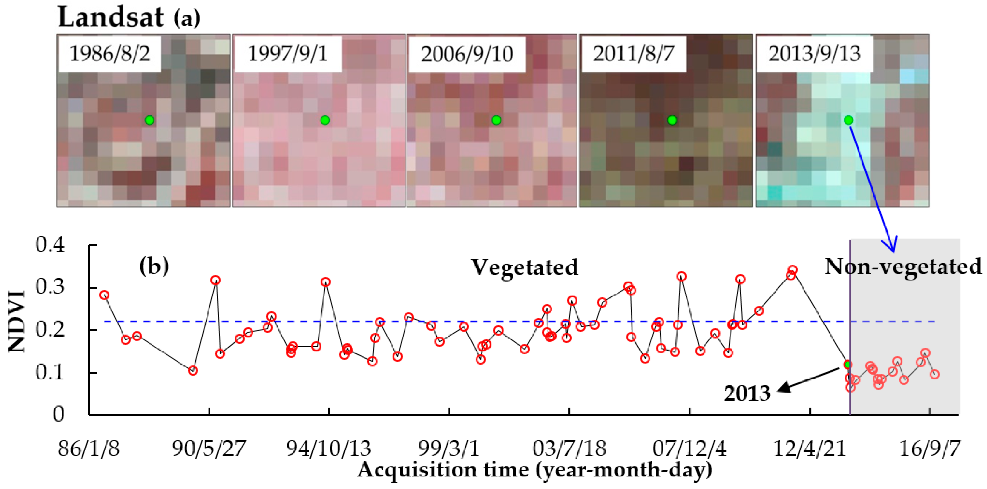
The ith observed NDVI value in the 1997–T₂ time series was compared with the simulated NDVI corresponding to the month and date of the observed NDVI in the intra-annual time series. The NDVI in this epoch was considered an anomaly flag if the difference between the observed and fitted values was more than three times the RMSE. Conversely, the intra-annual composite was updated dynamically with newly acquired NDVI observations using the method described in section (1).

(b)

Vegetation type change occurred for a given pixel if the change direction of the first anomaly flag was consistent with the other anomaly flags within three years, and there were at least three anomalies for different years within a six-year period. The year in which the first anomaly occurred was the potential year (T₃) of vegetation type change.

(c)

The iterative detection process was terminated if the rules for (a) and (b) were satisfied. Conversely, the (i + 1)th NDVI in the time series was analyzed continuously based on the previous rules. It was believed that vegetation type change had not occurred during the study period if no anomaly flag was revealed in the detection process.

Figure 7a–f displays the detection process for a sample pixel with a conversion from cropland to forest/grassland in 1997. Three anomalies were detected in three different years (1997, 1999, and 2002), and the year of the first anomaly (1997) was defined as the potential year of change of vegetation type.

2.4.3. Determination of Change Year and Change Direction for Forest/Grassland and Cropland

In this study, decision tree rules were developed to classify forest/grassland and cropland using NDVI time series from 1986 to 2016, as shown in Figure 8. The metrics and corresponding thresholds used in the decision tree were determined by analyzing a NDVI histogram of samples and repeated classification trails. It should be noted that the inter-annual change trend of time series is characterized by the significance level derived from the Mann-Kendall test [44] in this study.

If the year of vegetation type change is detected by the algorithm in Section 2.4.2, then the decision tree classification can be conducted separately for the NDVI time series in the periods before and after change has occurred. The year of vegetation type change is considered erroneous if the classified land cover remains the same, otherwise, the year of change is determined to be accurate.

Figure 9 displays the detection process for a pixel sample converted from cropland into forest/grassland in 2005, which was captured by multi-temporal high spatial resolution imagery (SPOT-5, GF-1, GE) (Figure 9a). The year of land cover change was detected using the detection algorithm in Section 2.4.2. (Figure 9b). Vegetation type was then classified in the two periods before and after the year of change, based on the decision tree rules in Section 2.4.3. as illustrated in Figure 9c–f. The year of change was determined to be 2005, which agrees with the change year identified by field survey data.

2.5. Accuracy Assessment of Contiuous Change Detection Algorithm

In this study, the spatial detection accuracy from 1986 to 2016 was evaluated by constructing an error matrix [45] of unchanged (FG, C, and NV) and changed land cover types (C–FG, C–NV, FG–C, FG–NV, NV–C, and NV–FG) based on 3919 validation samples (Table 1), and overall accuracy, kappa coefficient, user accuracy and producer accuracy were calculated for different change types. Additionally, an error tolerance of overall accuracy at a confidence level of 95% was calculated using the method proposed by Baraldi et al. [46] to illustrate the statistical significance of accuracy assessment. The temporal detection accuracy was evaluated based on the 489 pixel samples with real change time in Table 1. The temporal accuracy is characterized by the proportion of pixels that had different time deviations between the detection results and reference data [32].

In addition, two long-term time series were generated using annual maximum NDVI of GIMMS, and annual maximum LAI of GLASS during 1982–2013 for assessing the temporal accuracy of vegetation anomaly detected by the proposed method at large scale. Globland30 product was also compared with change detection results to illustrate the advantages of temporal and spatial accuracy of the proposed method at 30-m scale.

3. Results

3.1. Continuous Land Cover Detection Result from 1986 to 2016

In the study, continuous land cover classifications were generated for three land cover types (forest/grassland, cropland, and non-vegetated areas) from 1986 to 2016 using the proposed method. The land cover classification for 1986 and 2014, as well as the year of land cover change, are displayed in Figure 10. It was revealed that most of the sandy land in the Mu Us desert has been converted into forest/grassland, and most cropland in the loess hill and gully area was converted into forest/grassland.

Figure 11 displays a sub-region classification map for areas with a typical conversion from cropland into forest/grassland. The land cover in 1986 and 2014 cannot be identified only using bi-temporal images (Figure 11a,c), however, different land cover types for 1986 and 2014 and the year of land cover change were successfully detected using NDVI time series (Figure 11b,d,e).

A statistical analysis of area percentages for land cover types in each year is shown in Figure 12. The forest/grassland areas covered 30.5% of the total study area during 1986–1996, consequently, the area increased to 37.7% in 1997, and then 69.4% in 2002. Forest/grassland areas remained stable after 2002, and accounted for 71.6% of the study area in 2016. However, the percentage of cropland and non-vegetated areas in the study area was observed to decline during the study period.

3.2. Accuracy Validation of Continuous Change Detection Results

3.2.1. Direct Validation

The spatial accuracy of change detection during 1986–2016 is provided in

Table 2. Accuracy assessment of change detection result.

		Unchanged			Changed						UA (%)	UA (%)
Class		FG	C	NV	C-FG	C-NV	FG-C	FG-NV	NV-C	NV-FC
Unchanged	FG	329	36	0	31	0	10	5	0	8	78.5	92.1
	C	30	854	0	43	0	27	2	0	0	89.3
	NV	2	0	232	0	0	0	0	0	0	99.1
Changed	C-FG	27	64	0	1158	0	16	0	0	0	91.5	95.3
	C-NV	1	0	0	0	201	0	29	0	0	87.0
	FG-C	8	5	0	46	0	95	0	7	0	59.0
	FG-NV	0	0	0	0	27	0	165	0	0	85.9
	NV-C	0	1	0	0	0	0	0	52	4	91.2
	NV- FG	1	0	0	0	0	0	0	2	401	99.3
PA (%)		82.7	89.0	100.0	90.6	88.2	64.2	82.1	85.2	97.1
PA (%)		93.2			94.5
9 classes for changed and stable land cover classes: Overall accuracy = 88.9% ± 1.0%, Kappa = 0.86
2 classes for changed and unchanged classes: Overall accuracy = 94.0% ± 0.0%, Kappa = 0.88

FG: forest/grassland, C: cropland, NV: non-vegetation, C-FG: cropland > forest/grassland, C-NV: cropland > non-vegetation, FG-C: forest/grassland > cropland, FG-NV: forest/grassland > cropland, NV-C: non-vegetation > cropland. NV-FG: non-vegetation > forest/grassland.

. The overall accuracy was 94.0% ± 0.0%, with a kappa coefficient of 0.88, for two types of unchanged and changed land cover, respectively. The producer’s and user’s accuracy for both types was greater than 94%. The overall accuracy was 88.9% ± 1.0%, with a kappa coefficient of 0.86, for all nine types of unchanged and changed land cover. These results suggest that the accuracy of the proposed algorithm was satisfactory for detecting land cover change.

Non-vegetated areas had the highest producers’ and user’s accuracy (>99%) among the unchanged land cover types. The classification accuracies for forest/grassland and cropland were above 78%. Among the changed land cover types, the C–FG type was the most prominent type of land cover change in the study area. Both the producer’s accuracy and user’s accuracy for this type was above 90%. Conversely, the FG–C type had the lowest producer’s (59.0%) and user’s accuracy (64.2%). Both the C–NV and NV-FG conversion types had a high producer’s accuracy with 88.2% and 97.1%, respectively. Conversely, the FG-NV and NV-C types featured a lower producer’s accuracy with 82.1% and 85.2%, respectively.

The temporal accuracy of change detection was assessed using the 454 pixels with correct detection of change direction selected from samples with real change time, as illustrated in

Table 3. Accuracy assessment of change detection in the temporal domain (time deviation).

	Same Year	≤1 Year	≤2 Year	≤3 Year
Number of pixels	43	165	179	67
Proportion (%)	9.4	36.3	39.5	14.8

. The proportion of pixels that had the same year of change for the algorithm results and reference data was 9.4%. The proportion of pixels that had a 1-year, 2-year, and 3-year deviation between the algorithm results and reference data were 36.3%, 39.5%, and 14.8%, respectively. These results suggest that the year of land cover change was successfully retrieved using the proposed algorithm, with 85.2% of the change pixels having a discrepancy of less than 2 years.

3.2.2. Indirect Validation

It was shown that vegetation degradation in 1997 (Figure 13a) was captured by the long-term time series of GIMMS NDVI and GLASS LAI, while the dynamics of annual precipitation (Figure 13b) revealed that no abrupt changes of annual precipitation were observed during 1996–1997. Thus, the sudden vegetation degradation in 1997 can be attributed to vegetation change caused by intensive human activities rather than climate change. This proves that the change event for vegetation in 1997 (Figure 12) detected using the proposed algorithm, was indeed caused by land cover change, which lends some credibility to the overall temporal detection accuracy of vegetation type change at the large scale. Additionally, this historical vegetation change supports the hypothesis of the proposed algorithm, namely, that no significant change occurred in vegetation during 1986–1996.

Land cover change between 2000 and 2010 derived from Globeland30 and classifications by the proposed algorithm were compared, as shown in

Table 4. Comparative analysis of the land cover classification results for GlobeLand30 and the proposed algorithm.

Year	Area Proportion (%) of Each Land Cover Type in the Study Area
	Classification in This Study			GlobeLand30
	C	FG	NV	C	FG	NV
2000	37.1	47.2	15.7	42.4	53.9	3.7
2010	26.1	71.8	2.1	42.1	54.1	3.8

C: cropland, FG: forest/grassland, NV: non-vegetated.

. Results revealed that land cover was almost stable during 2000–2010 according to Globeland30, whereas the proposed algorithm better reflected actual changes of land cover in the context of the GFGP in the Loess Plateau. In the spatial domain, a high-resolution GE image (0.5 m) from May 2013 was used to evaluate the classification accuracy of cropland from Globeland30 and results from the proposed algorithm in 2010. Results indicated that GlobeLand30 mistakenly classified large areas of forest/grassland as cropland, and omitted some cropland areas, whereas the proposed algorithm was able to accurately identify croplands, especially in long, narrow terraced fields (Figure 14). Thus, the proposed algorithm provided a high level of spatial and temporal accuracy for identifying forest/grassland and cropland.

3.3. The Effect of Full Temporal Information on Spatial Detection Accuracy

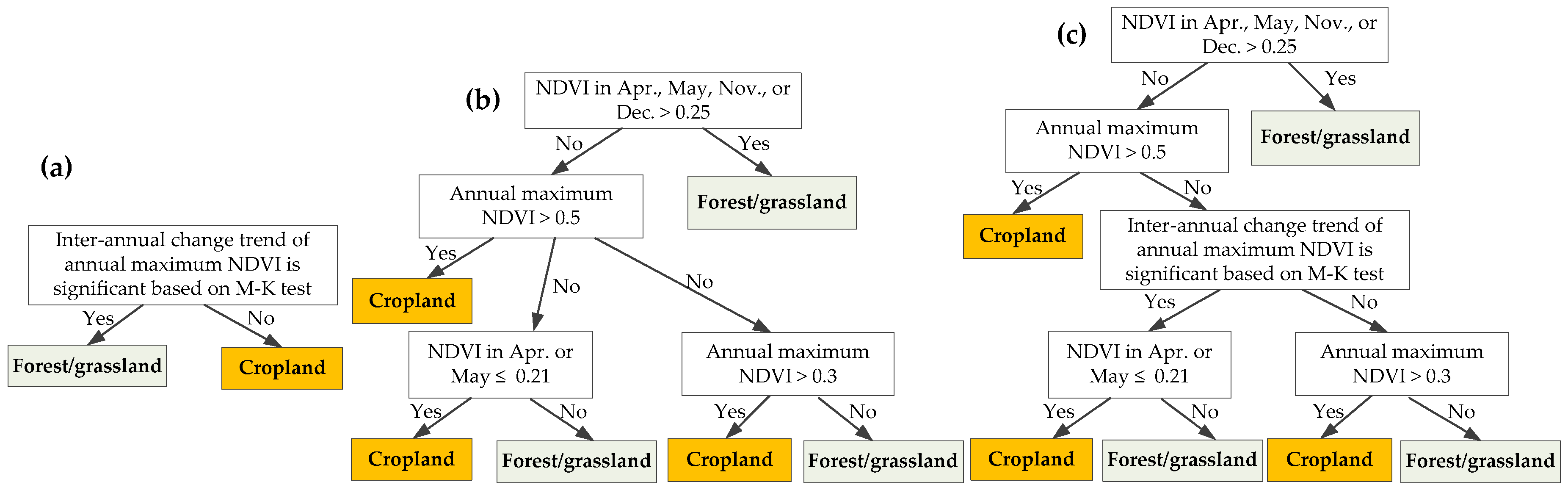
To illustrate the effect of full temporal information on vegetation type identification, the classification accuracies of four decision tree classifiers with different temporal information were compared, as below:

(a)

Decision tree using significance of change trend of annual maximum NDVI from multiple years;

(b)

Decision tree using multi-month NDVI from single year;

(c)

Decision tree using a combination of decision tree (a) and (b); and

(d)

Decision tree using a combination of decision tree (a) and multi-month NDVI from multiple years.

Figure 15 shows the first three decision trees which were derived from the optimal decision tree (decision tree (d)) presented in Section 2.4.3. Because there were no significant vegetation types changes since 2006, the multi-month NDVI from multiple years and inter-annual change trend were derived using NDVI time series from 2006–2016. Due to the discontinuity of Landsat observations, an intra-annual time series composite from 2013–2016 was able to provide complete multi-month NDVI in one year. 500 samples (1:1 for cropland and forest/grassland) were randomly generated from training samples with stable land cover after 2006, and were used for assessing the performances of four decision tree classifiers. The overall accuracy of the decision tree using multi-month data (73.3%) was superior to the inter-annual change trend (61.9%). The integrated temporal information also produced a better performance (80.5%). However, the decision tree using full temporal information (multi-month NDVI from multiple years) produced the highest overall accuracy (87.4%). A comparison of accuracies for the four decision tree classifiers suggests that rich temporal information is necessary for improving classification accuracy in the Loess Plateau.

3.4. The Effect of Removing False Detection on Temporal Detection Accuracy

In the proposed algorithm, it was considered to be a false detection if the change direction of the anomaly was not consistent with subsequent anomalies within a three year period. This effectively removes the false anomalies caused by factors such as clouds, cloud shadows, or fallowing. Additionally, if there were less than three anomalies in different years within a six-year period, these anomalies represented a transient change caused by an accidental event of rainfall or human activity instead of continuous change caused by actual land cover change.

The detection of false anomalies for a stable cropland sample is displayed in Figure 16. The anomalies occurred in many years, as illustrated in Figure 16b,c. However, these false NDVI anomalies were detected based on the detection rules of the proposed algorithm. This is very helpful to reduce the influence of various factors on vegetation types change detection for the Loess Plateau, including clouds, cloud shadows, precipitation and human activity.

However, the algorithm still produces some false detection when using complex and diverse NDVI time series in practical application. False detections can be reduced further by analyzing classified land cover before and after change. Figure 17 shows that a pixel sample of stable cropland had a potential change in 2004 according to the detection results (Figure 17b). However, the same vegetation type was identified before and after the change, suggesting that the potential change year was false detection and the land cover was stable (Figure 17c–f), which was validated by multi-temporal high resolution imagery (Figure 17a).

4. Discussion

4.1. Application of Intra-Annual NDVI Time Series Composite Method

In this study, an intra-annual NDVI time series composite method was proposed based on the hypothesis that no obvious change in forest/grassland and cropland had occurred in the study area during a period of time. Because changes in phenological characteristics for a specific vegetation type is generally slight over time, all available Landsat observations during this period of time can be employed to reconstruct a complete and continuous intra-annual NDVI time series, as illustrated in Figure 6. An obvious phenological characteristic is present after reconstructing the intra-annual NDVI time series, which is helpful for characterizing vegetation types.

Although this composite method can overcome the disadvantages of temporal resolution of Landsat acquisitions to detect vegetation type change, practical application is still subject to the duration of stable periods of land cover and the number of available Landsat images. A longer period of stable land cover type suggests a higher likelihood of acquiring sufficient satellite observations, and vice versa. The duration of the period can be shortened when satellite observations are appropriate. A shorter stable period and insufficient satellite observations can make it difficult for this method to function effectively. Therefore, the proposed intra-annual NDVI time series composite method can be applied to arid and semi-arid areas with enough Landsat observations and a historical period when land cover was almost stable, which suggests that it is suitable for application in northwest China, especially for the Loess Plateau.

4.2. Underlying Mechanism of Determining Classification Metrics and Thresholds

In the Loess Plateau, crops are sowed in April-May and are harvested before November, hence the greenness of cropland is definitely low in April, May, November, and December, which suggests that the vegetation with a high level of greenness in these months must be forest/grassland. Therefore, a threshold (0.25) of NDVI in any of these months was determined to identify forest/grassland. Cropland greenness is typically characterized by relatively high seasonal variation, thus a combination of NDVI thresholds from different seasons, namely that a high (>0.5) annual maximum NDVI and a low NDVI (<0.25) in April and May was used to identify cropland. However, these rules are not effective for the vegetated pixels that have similar intra-annual NDVI characteristics. To solve this problem, we used the inter-annual change trend of annual maximum NDVI to classify the remaining pixels on the basis that vegetation greenness has an obvious increasing trend after GFGP implementation for most forest/grassland, whereas cropland greenness is relatively stable. Consequently, forest/grassland with insignificant inter-annual change was extracted from cropland using an NDVI threshold (0.3) of annual maximum, and cropland with significant inter-annual change was extracted from forest/grassland using an NDVI threshold (0.21) in April and May. Additionally, multi-year criterion in the decision tree is helpful to guarantee that satisfying the rules is not an accidental event caused by rainfall or anthropogenic factors, thus improving the final classification accuracy.

In practice, there is no universally applicable threshold in all regions of the world for any algorithm, and the thresholds of detection algorithms are always trained by available samples within the targeted study area. Therefore, the thresholds determined in this study might be different when using more samples from the whole Loess Plateau, however, they still have important reference value for the areas without sufficient samples.

4.3. Source of Detection Error

In this study, the change time of land cover detected by the proposed algorithm is earlier or later than the real change year. Some of the reasons for the time discrepancy were consistent with the conclusion drawn by Zhu et al. [32]. It should be noted that vegetation change resulting from precipitation and human activity (e.g., rainstorm, fallowing and grazing) is also an important reason leading to the earlier discrepancy in detected change time. The assessment of change types (Table 2) revealed that the proposed algorithm performed more accurately in identifying cropland than forest/grassland in the period before land cover change, whereas a contrary situation was observed in later change periods. This primarily occurred because vegetation was influenced by intense human activity (such as grazing and reclamation) in the period before the GFGP. Forest/grassland vegetation coverage remained at low levels, which led to less obvious inter-annual and intra-annual NDVI variation characteristics. However, the phenological characteristics for crops were more likely to be captured by satellite observations. This explains why cropland vegetation had a lower omission error during this period. Forest/grassland coverage exhibited a significant increase in the later stages after the GFGP was implemented. As a result, the inter-annual and intra-annual NDVI variation characteristics for forest/grassland were more likely to be captured by satellite observations, which resulted in forest/grassland having a lower omission error during later periods. However, because C-FG conversion is the dominant type of land cover change in the Loess Plateau, the different performances of the proposed algorithm for different periods only had a slight effect on the accuracy of the change detection application in the Loess Plateau.

5. Conclusions

Continuous detection of the change in land cover in the Loess Plateau has proved to be difficult using medium-resolution remote sensing imagery. A new algorithm for detecting the continuous dynamics of forest/grassland and cropland was developed in this study. An intra-annual NDVI time series composite method was proposed to fully utilize available Landsat data. Additionally, continuous change detection rules and classification rules for forest/grassland and cropland were developed to achieve land cover classification maps for each year. Results revealed that the proposed algorithm was accurate in identifying land cover change, with an overall accuracy of 88.9% and a kappa coefficient of 0.86. The time of the land cover change was also successfully retrieved, with 85.2% of the change pixels having a discrepancy of less than two years.

For this algorithm, the change detection rules considering the persistent effect of vegetation type change to vegetation greenness and the classification metrics involving inter-annual and intra-annual temporal information are very critical for improving the temporal and spatial accuracy of change detection results. The framework of the proposed algorithm has a significant application in developing a continuous change detection algorithm of vegetation dynamics in arid and semi-arid areas where vegetation growth is sensitive to climate and anthropogenic factors, especially for the Loess Plateau.

The present study requires further investigation due to various reasons. Firstly, the sample data obtained in this study did not have adequate spatial representation, especially for the timing of land cover change. Therefore, a comprehensive sample database should be constructed in future studies. Additionally, only three land cover types (e.g., forest/grassland, cropland, and non-vegetated areas) were involved in this study. Other land cover types should be taken into consideration in future studies in order to implement continuous change detection for more diversified types of land cover. Lastly, multi-sensor data, including Landsat-8, Sentinel-2, and HJ-1 should be integrated to increase the temporal information gathered from time-series observations acquired by different satellites. Such data can improve the continuous dynamic change monitoring accuracy for land cover.

References

1. Liu, J.G.; Diamond, J. China’s environment in a globalizing world. Nature 2005, 435, 1179–1186. [Google Scholar] [CrossRef] [PubMed]
2. Zhang, Y.; Peng, C.H.; Li, W.Z.; Tian, L.X.; Zhu, Q.A.; Chen, H.; Fang, X.Q.; Zhang, G.L.; Liu, G.B.; Mu, X.M.; et al. Multiple afforestation programs accelerate the greenness in the ‘Three North’ region of China from 1982 to 2013. Ecol. Indic. 2016, 61, 404–412. [Google Scholar] [CrossRef] [Green Version]
3. Wu, Z.T.; Wu, J.J.; Liu, J.H.; He, B.; Lei, T.J.; Wang, Q.F. Increasing terrestrial vegetation activity of ecological restoration program in the Beijing–Tianjin Sand Source Region of China. Ecol. Eng. 2013, 52, 37–50. [Google Scholar] [CrossRef]
4. Yin, R.S.; Yin, G.P. China’s primary programs of terrestrial ecosystem restoration: Initiation, implementation, and challenges. Environ. Manag. 2010, 45, 429–441. [Google Scholar] [CrossRef] [PubMed]
5. Liu, D.; Chen, Y.; Cai, W.W.; Dong, W.J.; Xiao, J.F.; Chen, J.Q.; Zhang, H.C.; Xia, J.Z.; Yuan, W.P. The contribution of China’s Grain to Green Program to carbon sequestration. Landsc. Ecol. 2014, 29, 1675–1688. [Google Scholar] [CrossRef]
6. Zheng, F.L. Effect of vegetation changes on soil erosion on the Loess Plateau. Pedosphere 2006, 16, 420–427. [Google Scholar] [CrossRef]
7. Zhao, A.Z.; Zhang, A.B.; Lu, C.Y.; Wang, D.L.; Wang, H.F.; Liu, H.X. Spatiotemporal variation of vegetation coverage before and after implementation of Grain for Green Program in Loess Plateau, China. Ecol. Eng. 2017, 104, 13–22. [Google Scholar] [CrossRef]
8. Luo, Y.; Yang, S.T.; Liu, X.Y.; Liu, C.M.; Song, W.L.; Dong, G.T.; Zhao, H.G.; Lou, H.Z. Land use change in the reach from Hekouzhen to Tongguan of the Yellow River during 1998–2010. Acta Geogr. Sin. 2014, 69, 42–53. (In Chinese) [Google Scholar]
9. Wang, S.; Fu, B.J.; Piao, S.L.; Lü, Y.H.; Ciais, P.; Feng, X.M.; Wang, Y.F. Reduced sediment transport in the Yellow River due to anthropogenic changes. Nat. Geosci. 2017, 9, 38–41. [Google Scholar] [CrossRef]
10. Liu, X.Y.; Yang, S.T.; Jin, S.Y.; Luo, Y.; Zhou, X. The method to evaluate the sediment reduction from forest and grass land cover large area in the Loss hilly area. J. Hydraul. Eng. 2014, 45, 135–141. (In Chinese) [Google Scholar]
11. Liu, X.Y.; Liu, C.M.; Yang, S.T.; Jin, S.Y.; Gao, Y.J.; Gao, Y.F. Influences of shrubs-herbs-arbor vegetation coverage on the runoff based on the remote sensing data in Loess Plateau. Acta Geogr. Sin. 2014, 69, 1595–1603. (In Chinese) [Google Scholar]
12. Wang, S.; Fu, B.J.; Liang, W.; Liu, Y.; Wang, Y.F. Driving forces of changes in the water and sediment relationship in the Yellow River. Sci. Total Environ. 2017, 576, 453–461. [Google Scholar] [CrossRef] [PubMed]
13. Dissmeyer, G.E.; Foster, G.R. Estimating the cover-management factor (C) in the Universal Soil Loss Equation for forest conditions. J. Soil Water Conserv. 1981, 36, 235–240. [Google Scholar]
14. Zhang, H.D.; Zhang, R.H.; Qi, F.; Liu, X.; Niu, Y.; Fan, Z.F.; Zhang, Q.H.; Li, J.Z.; Yuan, L.; Song, Y.Y.; et al. The CSLE model based soil erosion prediction: Comparisons of sampling density and extrapolation method at the county level. Catena 2018, 165, 465–472. [Google Scholar] [CrossRef]
15. Karydas, C.G.; Panagos, P. Modelling monthly soil losses and sediment yields in Cyprus. Int. J. Digit. Earth 2016, 9, 766–787. [Google Scholar] [CrossRef]
16. Odongo, V.O.; Onyando, J.O.; Mutua, B.M.; Vanoel, P.R.; Becht, R. Sensitivity analysis and calibration of the Modified Universal Soil Loss Equation (MUSLE) for the upper Malewa Catchment, Kenya. Int. J. Sediment Res. 2013, 28, 368–383. [Google Scholar] [CrossRef]
17. Phiri, D.; Morgenroth, J. Developments in Landsat Land Cover Classification Methods: A Review. Remote Sens. 2017, 9, 967. [Google Scholar] [CrossRef]
18. Liu, L.Y. Opportunities of Mapping Forest Carbon Stock and its Annual Increment Using Landsat Time-Series Data. Geoinform. Geostat. Overv. 2016, 4, 1000151. [Google Scholar] [CrossRef]
19. Townshend, J.R.; Masek, J.G.; Huang, C.Q.; Vermote, E.F.; Gao, F.; Channan, S.; Sexton, J.O.; Feng, M.; Narasimhan, R.; Kim, D.; et al. Global characterization and monitoring of forest cover using Landsat data: Opportunities and challenges. Int. J. Digit. Earth 2012, 5, 373–397. [Google Scholar] [CrossRef]
20. Toure, S.I.; Stow, D.A.; Shih, H.C.; Weeks, J.; Lopez-Carr, D. Land cover and land use change analysis using multi-spatial resolution data and object-based image analysis. Remote Sens. Environ. 2018, 210, 259–268. [Google Scholar] [CrossRef]
21. Wohlfart, C.; Liu, G.H.; Huang, C.; Kuenzer, C. A River Basin over the Course of Time: Multi-Temporal Analyses of Land Surface Dynamics in the Yellow River Basin (China) Based on Medium Resolution Remote Sensing Data. Remote Sens. 2016, 8, 186. [Google Scholar] [CrossRef] [Green Version]
22. Huang, C.Q.; Goward, S.N.; Masek, J.G.; Thomas, N.; Zhu, Z.L.; Vogelmann, J.E. An automated approach for reconstructing recent forest disturbance history using dense Landsat time series stacks. Remote Sens. Environ. 2010, 114, 183–198. [Google Scholar] [CrossRef]
23. Li, M.S.; Huang, C.Q.; Zhu, Z.L.; Wen, W.S.; Xu, D.; Liu, A.X. Use of remote sensing coupled with a vegetation change tracker model to assess rates of forest change and fragmentation in Mississippi, USA. Int. J. Remote Sens. 2009, 30, 6559–6574. [Google Scholar] [CrossRef]
24. Liu, L.; Tang, H.; Caccetta, P.; Lehmann, E.A.; Hu, Y.; Wu, X. Mapping afforestation and deforestation from 1974 to 2012 using Landsat time-series stacks in Yulin District, a key region of the Three-North Shelter region, China. Environ. Monit. Assess. 2013, 185, 9949–9965. [Google Scholar] [CrossRef] [PubMed]
25. Zhu, C.; Lu, D.S.; Victoria, D.; Dutra, L.V. Mapping Fractional Cropland Distribution in Mato Grosso, Brazil Using Time Series MODIS Enhanced Vegetation Index and Landsat Thematic Mapper Data. Remote Sens. 2016, 8, 22. [Google Scholar] [CrossRef]
26. Neigh, C.S.; Bolton, D.K.; Diabate, M.; Williams, J.J.; Carvalhais, N. An Automated Approach to Map the History of Forest Disturbance from Insect Mortality and Harvest with Landsat Time-Series Data. Remote Sens. 2014, 6, 2782–2808. [Google Scholar] [CrossRef] [Green Version]
27. Liu, S.S.; Wei, X.L.; Li, D.Q.; Lu, D.S. Examining Forest Disturbance and Recovery in the Subtropical Forest Region of Zhejiang Province Using Landsat Time-Series Data. Remote Sens. 2017, 9, 479. [Google Scholar] [CrossRef]
28. Kennedy, R.E.; Cohen, W.B.; Schroeder, T.A. Trajectory-based change detection for automated characterization of forest disturbance dynamics. Remote Sens. Environ. 2007, 110, 370–386. [Google Scholar] [CrossRef]
29. Healey, S.P.; Cohen, W.B.; Yang, Z.Q.; Krankina, O.N. Comparison of Tasseled Cap-based Landsat data structures for use in forest disturbance detection. Remote Sens. Environ. 2005, 97, 301–310. [Google Scholar] [CrossRef]
30. Beurs, K.M.D.; Owsley, B.C.; Julian, J.P. Disturbance analyses of forests and grasslands with MODIS and Landsat in New Zealand. Int. J. Appl. Earth Obs. 2016, 45, 42–54. [Google Scholar] [CrossRef]
31. Hamunyela, E.; Reiche, J.; Verbesselt, J.; Herold, M. Using Space-Time Features to Improve Detection of Forest Disturbances from Landsat Time Series. Remote Sens. 2017, 9, 515. [Google Scholar] [CrossRef]
32. Zhu, Z.; Woodcock, C.E. Continuous change detection and classification of land cover using all available Landsat data. Remote Sens. Environ. 2014, 144, 152–171. [Google Scholar] [CrossRef]
33. Zhu, Z.; Wang, S.H.; Woodcock, C.E. Improvement and Expansion of the Fmask Algorithm: Cloud, Cloud Shadow, and Snow Detection for Landsats 4–7, 8, and Sentinel 2 images. Remote Sens. Environ. 2015, 159, 269–277. [Google Scholar] [CrossRef]
34. Hu, Y.; Liu, L.Y.; Liu, L.L.; Peng, D.L.; Jiao, Q.J.; Zhao, H. A Landsat-5 Atmospheric Correction Based on MODIS Atmosphere Products and 6S Model. IEEE J. Sel. Top. Appl. Earth Obs. Remote Sens. 2014, 7, 1609–1615. [Google Scholar] [CrossRef]
35. Berk, A.; Bernstein, L.S.; Anderson, G.P.; Acharya, P.K.; Robertson, D.C. MODTRAN cloud and multiple scattering upgrades with application to AVIRIS. Remote Sens. Environ. 1998, 65, 367–375. [Google Scholar] [CrossRef]
36. Teillet, P.M.; Guindon, B.; Goodenough, D.G. On the slope-aspect correction of multispectral scanner data. Can. J. Remote Sens. 1982, 8, 84–106. [Google Scholar] [CrossRef]
37. He, Y.Q.; Lee, E.; Warner, T.A. A time series of annual land use and land cover maps of China from 1982 to 2013 generated using AVHRR GIMMS NDVI3g data. Remote Sens. Environ. 2017, 199, 201–217. [Google Scholar] [CrossRef]
38. Xiao, Z.Q.; Liang, S.L.; Sun, R.; Wang, J.D.; Jiang, B. Estimating the fraction of absorbed photosynthetically active radiation from the MODIS data based GLASS leaf area index product. Remote Sens. Environ. 2015, 171, 105–117. [Google Scholar] [CrossRef]
39. Zhang, W.Q.; Chen, J.; Liao, A.P.; Han, G.; Chen, X.H.; Chen, L.J.; Peng, S. Geospatial knowledge-based verification and improvement of GlobeLand30. Sci. China Earth Sci. 2016, 59, 1–11. [Google Scholar] [CrossRef]
40. Tucker, C.J. Red and photographic infrared linear combinations for monitoring vegetation. Remote Sens. Environ. 1979, 8, 127–150. [Google Scholar] [CrossRef] [Green Version]
41. Cheng, W.C.; Chang, J.C.; Chang, C.P.; Su, Y.; Tu, T.M. A Fixed-Threshold Approach to Generate High-Resolution Vegetation Maps for IKONOS Imagery. Sensors 2008, 8, 4308–4317. [Google Scholar] [CrossRef] [PubMed] [Green Version]
42. Han, N.; Wu, J.; Tahmassebia, A.R.S.; Xu, H.W.; Wang, K. NDVI-Based Lacunarity Texture for Improving Identification of Torreya Using Object-Oriented Method. Agric. Sci. China 2011, 10, 1431–1444. [Google Scholar] [CrossRef]
43. Savitzky, A.; Golay, M.J.E. Smoothing and Differentiation of Data by Simplified Least Squares Procedures. Anal. Chem. 1964, 36, 1627–1639. [Google Scholar] [CrossRef]
44. Liu, Y.L.; Wang, Q.; Bi, J.Z.; Zhang, M.M.; Xing, Q.G.; Shi, P. The analysis of NDVI trends in the coastal zone based on Mann-Kendall test: A case in the Jiaodong Peninsula. Acta Geogr. Sin. 2010, 32, 79–87. (In Chinese) [Google Scholar]
45. Lewis, H.G.; Brown, M. A generalized confusion matrix for assessing area estimates from remotely sensed data. Int. J. Remote Sens. 2001, 22, 3223–3235. [Google Scholar] [CrossRef] [Green Version]
46. Baraldi, A.; Puzzolo, V.; Blonda, P.; Bruzzone, L.; Tarantino, C. Automatic Spectral Rule-Based Preliminary Mapping of Calibrated Landsat TM and ETM+ Images. IEEE Trans. Geosci. Remote Sens. 2006, 44, 2563–2586. [Google Scholar] [CrossRef] [Green Version]
Figure 1. (a) Topographical map of the Loess Plateau in northern China; (b) accumulated rainfall anomaly from 1986 to 2016; (c) Landsat8 OLI image of the study area (30 July 2014, RGB:742) showing the 118 field survey sites.
Remotesensing 10 01775 g001
Figure 2. (a) Dates for Landsat time-series imagery acquired for this study; (b) spatial distribution of the numbers of pixel-scale Landsat clear observations (without cloud/cloud shadows) from 1986 to 2016.
Remotesensing 10 01775 g002
Figure 3. Photographs of four field sites taken on 27 May 2017: (a) woodland, (b) mosaic shrub/grassland, (c) sparse grassland, and (d) cropland.
Remotesensing 10 01775 g003
Figure 4. Flowchart of the forest/grassland and cropland dynamic detection algorithm based on the Landsat NDVI time series. Note: RMSE, root mean square error; T1, time 1; T2, time 2; T3, time 3; i, the ith epoch from 1997 to T2.
Remotesensing 10 01775 g004
Figure 5. (a) Multi-temporal Landsat surface reflectance images (RGB:432); (b) NDVI time series for vegetated to non-vegetated pixel.
Remotesensing 10 01775 g005
Figure 6. (a) Original NDVI time series from 1986 to 1996; (b) reconstructed intra-annual NDVI time series for irrigated cropland pixel.
Remotesensing 10 01775 g006
Figure 7. Detection process for the potential change year of vegetation type for pixel sample with a conversion from cropland to forest/grassland in 1997: (a) intra-annual time series during 1986–1996, (b) first anomaly in 1997, (c) intra-annual time series during 1986–1998, (d) second anomaly detected in 1999, (e) intra-annual time series during 1986–2001, (f) third anomaly detected in 2002. Note: red circle, observed NDVI; green solid circle, anomalous NDVI.
Remotesensing 10 01775 g007
Figure 8. Decision tree classification rules for forest/grassland and cropland in the loess hill and gully areas.
Remotesensing 10 01775 g008
Figure 9. The detection process for the pixel sample showing conversion from cropland into forest/grassland in 2005. (a) high-resolution images of SPOT-5, GF-1, and GE; (b) year of vegetation type change (2005) detected by the proposed algorithm; (c) intra-annual NDVI time series composite from 1986–2004; (d) inter-annual time series of annual maximum NDVI from 1986–2004; (e) intra-annual NDVI time-series composite from 2005–2016; (f) inter-annual time series of annual maximum NDVI from 2005–2016. Note: red circle, observed NDVI; blue line, NDVI threshold for 0.21, 0.25 and 0.5; dash line, inter annual change trend of time series.
Remotesensing 10 01775 g009aRemotesensing 10 01775 g009b
Figure 10. (a) 1986 Landsat image (RGB:742); (b) 1986 land cover classification map; (c) 2014 Landsat image (RGB:742); (d) 2014 land cover classification map; (e) spatial distribution of the change year of land cover types for each pixel.
Remotesensing 10 01775 g010
Figure 11. (a) 1986 Landsat image (RGB:742); (b) 1986 land cover classification map; (c) 2014 Landsat image (RGB:742); (d) 2014 land cover classification map; (e) spatial distribution map of the year when land cover change occurred for each pixel. Graphs (1) and (2) indicate the dynamic changes of NDVI time series for the two pixels (central pixel in location 1 and 2) with a conversion from cropland into forest/grassland occurred in 2005 and 1997.
Remotesensing 10 01775 g011aRemotesensing 10 01775 g011b
Figure 12. Percentage of area for forest/grassland (FG), cropland (C), and non-vegetated (NV) land cover types during 1986–2016.
Remotesensing 10 01775 g012
Figure 13. (a) Time-series of the annual maximum NDVI from GIMMS NDVI3g, and the annual maximum LAI from GLASS LAI during 1982–2013; (b) variations in annual precipitation provided by the Hengshan Meteorological Station.
Remotesensing 10 01775 g013
Figure 14. (a) Classified cropland of GlobeLand30 in 2010 overlaid on high-resolution GE imagery; (b) GE imagery in May 2013; (c) classified cropland generated by the proposed algorithm in 2010 overlaid on high-resolution GE imagery; (d) sub-regional map of (a); (e) sub-regional map of (c).
Remotesensing 10 01775 g014
Figure 15. (a) Decision tree with inter-annual time series of annual maximum NDVI during 2006–2016; (b) decision tree with a multi-month NDVI during 2013–2016 and without multi-year criteria; (c) decision tree with the combination of (a,b).
Remotesensing 10 01775 g015
Figure 16. Detection of false anomalies for a pixel sample of cropland: (a) original NDVI time series for the study period; (b) false anomalies detected by the proposed algorithm in 1999 and 2004; (c) false anomalies detected by the proposed algorithm in 2004, 2005, and 2006.
Remotesensing 10 01775 g016
Figure 17. The detection process for a pixel sample of stable cropland, (a) High-resolution images of SPOT-5, GF-1, and GE; (b) year of vegetation type change (2004) detected by the proposed algorithm; (c) intra-annual NDVI time series composite during 1986–2003; (d) inter-annual time series of annual maximum NDVI during 1986–2003; (e) intra-annual NDVI time-series composite during 2004–2016; (f) inter-annual time series of annual maximum NDVI during 2004–2016. Note: blue line, NDVI threshold for 0.21, 0.25 and 0.5; dash line, inter annual change trend of time series.
Remotesensing 10 01775 g017aRemotesensing 10 01775 g017b