Abstract
Accurate measurement of the field leaf area index (LAI) is crucial for assessing forest growth and health status. Three-dimensional (3-D) structural information of trees from terrestrial laser scanning (TLS) have information loss to various extents because of the occlusion by canopy parts. The data with higher loss, regarded as poor-quality data, heavily hampers the estimation accuracy of LAI. Multi-location scanning, which proved effective in reducing the occlusion effects in other forests, is hard to carry out in the mangrove forest due to the difficulty of moving between mangrove trees. As a result, the quality of point cloud data (PCD) varies among plots in mangrove forests. To improve retrieval accuracy of mangrove LAI, it is essential to select only the high-quality data. Several previous studies have evaluated the regions of occlusion through the consideration of laser pulses trajectories. However, the model is highly susceptible to the indeterminate profile of complete vegetation object and computationally intensive. Therefore, this study developed a new index (vegetation horizontal occlusion index, VHOI) by combining unmanned aerial vehicle (UAV) imagery and TLS data to quantify TLS data quality. VHOI is asymptotic to 0.0 with increasing data quality. In order to test our new index, the VHOI values of 102 plots with a radius of 5 m were calculated with TLS data and UAV image. The results showed that VHOI had a strong linear relationship with estimation accuracy of LAI (R2 = 0.72, RMSE = 0.137). In addition, as TLS data were selected by VHOI less than different thresholds (1.0, 0.9, …, 0.1), the number of remaining plots decreased while the agreement between LAI derived from TLS and field-measured LAI was improved. When the VHOI threshold is 0.3, the optimal trade-off is reached between the number of plots and LAI measurement accuracy (R2 = 0.67). To sum up, VHOI can be used as an index to select high-quality data for accurately measuring mangrove LAI and the suggested threshold is 0.30.
1. Introduction
Leaf area index (LAI), defined as half of the total leaf area per unit ground surface area [1], serves as a key indicator of carbon and nutrient cycling, rates of energy exchange between plants and the atmosphere, and ecological processes such as photosynthesis and transpiration [2,3,4]. The ability of LAI to characterize canopy structure is crucial for understanding the significant role LAI plays in assessing the health status [5,6,7], predicting future growth, and the production of mangrove forests [8,9].
The traditional ground-based measurements of LAI can be generally divided into two categories: direct methods and indirect methods. The direct methods mainly include destructive sampling [10,11], litterfall collection [12] and intercept point sampling [13]. Although the direct methods are known to be more accurate than the indirect ones, their being extremely costly, time-consuming and labor-intensive is disadvantageous and impractical in field conditions. The indirect methods in situ involve specially designed optical instruments, such as hemispherical photography [14,15] and LI-COR’s Plant Canopy Analyzer [16,17,18], which retrieve LAI based on gap fraction that is defined as the probability of light passing through the forest canopy without being blocked by foliage [19]. These indirect in situ methods provide accurate LAI measurement with easy and quick operation. However, they are susceptible to sky illumination and weather conditions, limiting the time flexibility [14,16,20].
In recent years, terrestrial laser scanning (TLS) has drawn increased attention as an innovative solution to overcome the limitations of traditional ground-based LAI measurements because of its low sensitivity to sky illumination and weather conditions [19]. The ability of TLS technology to characterize detailed three-dimensional (3-D) vegetation structure has offered the convenience to accurately retrieve LAI in various forests, such as shrub [10,13] and boreal forests [14,21,22,23], providing reference data for LAI estimation using spaceborne and airborne datasets [17,24,25]. Point cloud data (PCD) with complete or near-complete 3D information, regarded as high-quality data, is fundamental for accurately measuring forest LAI at plot scale [20]. However, occlusion of the laser beams by plant parts causes information loss to various extents during TLS data acquisition. As a result, existence of PCD with high information loss (i.e., poor-quality data) severely hampers the LAI measurement accuracy.
The occlusion effect can be ameliorated by an effective scanning set-up, such as multi-location scanning [10] and the bottom-up hemispherical central scanning [20]. However, it cannot be completely eliminated. No matter how TLS station is set up in the forest, some regions of occlusion still exists, especially in the dense and complex forest [26]. The occlusion problem is even more severe in mangrove forests. Mangrove forests constitute important intertidal ecosystems [4,6,27,28,29]. Mangrove trees often grow in high density and have complex root systems [30,31,32]. These characteristics result in difficulties of moving through dense stands and general inaccessibility over many areas [8]. As a result, locations where the TLS equipment can be placed are extremely limited, which worsens the occlusion problem [9,10,33]. Consequently, the TLS PCD contains a small amount high-quality data and massive poor-quality data. Therefore, it is necessary to assess data quality and screen out the poor-quality data.
Several previous studies have shown that regions of occlusion can be evaluated by computing the complete trajectories of laser pulses [25,26,34,35]. The occlusion effect is represented by the extent of the occluded regions, which is the accumulated volume of voxel with no record of any interactions with pulse and voxel. However, the pulse trajectory model to assess the regions of occlusion has two deficiencies. First, the profile of complete vegetation object cannot be determined. To this problem, incorporating optical imagery is a solution. Optical images explicitly describe the horizontal cover, and thus provide information to clearly define canopy boundaries. In order to maintain the precision that TLS provides, high spatial resolution imagery is required. Unmanned aerial vehicle (UAV) platforms can acquire images with centimeter level spatial resolution at very low cost and flexible times [36,37,38,39]. Second, the pulse trajectory model is computationally intensive because the model involves 3-D processing, which needs to directly manipulate large PCD [20]. Compared with the 3-D model, a model based on 2-D processing is easy to implement while intuitively reflecting horizontal occlusion.
This study aims to design a new approach to assess TLS data quality and retain high-quality data for mangrove LAI retrieval. The objectives of the research are three-fold: (1) to develop a vegetation horizontal occlusion index (VHOI) using the horizontal structural information of TLS PCD and UAV image; (2) to explore the ability of VHOI to quantitatively represent PCD quality; (3) to develop a threshold selection method for PCD filtering and suggest a VHOI threshold in mangrove LAI retrieval. Ultimately, we expect that VHOI is the assessment means for accurate estimation of not only mangrove LAI, but also other forests, and even other parameters such as biomass.
2. Materials
2.1. Study Area
The study site is located in the Dandou sea mangrove forest at 21°30′N–21°37′N and 109°37′E–109°40′E, which belongs to Shankou Mangrove National Nature Reserve. The study area consists of four mangrove species: Avicennia marina (AM), Aegiceras corniculatum (AC), Kandelia candel (KC), and Rhizophora stylosa (RS). The AM population is the largest, followed by AC, KC and a small amount of RS. The mangrove has two characteristics, shown in Figure 1a. On the one hand, the plants are extremely dense, making it inconvenient to move through them. On the other hand, the height of the mangrove is not high. The average height of the first three species is approximately 2.5 m, and the last one is approximately 3 m. Thus, the mangrove can be considered as “shrub-type” mangroves in this study site.
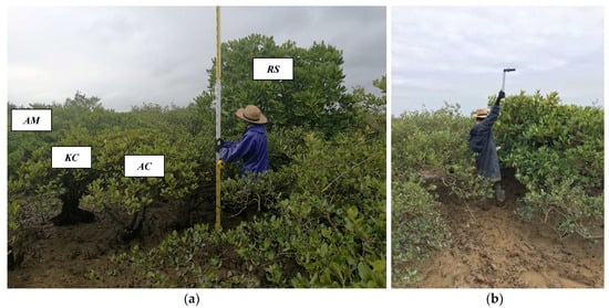
Figure 1.
(a) Four species of mangrove in the study area; (b) Researcher is acquiring field-measured leaf area index (LAI) data at plot scale with the radius of 5 m by the LAI-2200 Plant Canopy Analyzer.
2.2. Field Measurements
The field-measured LAI of the mangrove forest was measured using an LAI-2200 Plant Canopy Analyzer (PCA, Li-Cor Bioscience, Lincoln, NE, USA) at plot scale in June 2017, as shown in Figure 1b. Two principles of field-measured LAI were followed: (1) the field measurement of both dense and sparse mangrove was all conducted to ensure the quality of the representative; (2) the size of each plot was close to the optimal scale for mangrove LAI estimation at plot scale, which has been proven by some studies [4,7]. A total of 51 plots with a radius of 5 m were investigated. The working principle of PCA is that the light intensity from five zenith angles (7°, 23°, 38°, 53°, 68°) above and below the canopy was measured through a “fish-eye” optical sensor. The canopy structure parameters, such as LAI and gap fraction, were constructed using the radiative transfer model. To obtain the field-measured LAI, we first used a differential GPS with centimeter level accuracy to obtain accurate positions and determine the center point of the plot. Next, a 180° shading cover for the fisheye lens of the LAI equipment was used to reduce the influence of the surveyor on the measurement. The mean of the six LAI values every 60° were recorded for each plot. Each plot was measured three times, taking the mean of the three values as the LAI value of this plot. The distance is approximately 10 cm from the lens to the ground. In addition, the tree heights, species, and corresponding photos for each plot were recorded.
3. Methods
The following paragraphs schematically represent the overview of the different steps of our experiment in Figure 2.
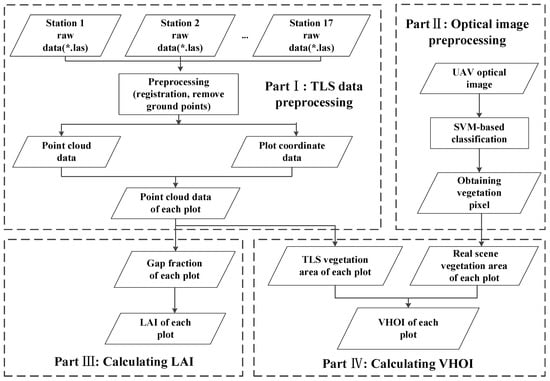
Figure 2.
Schematic representation to example the different steps for retrieving LAI and vegetation horizontal occlusion index (VHOI).
3.1. TLS Data Collection and Preprocessing
The TLS raw data were captured with Stonex X300 (Stonex Co., Ltd, Monza, Italy) on 2 June 2017. We set up a total of 17 scanning stations in the region. To guarantee mangrove LAI unaffected by the invasion species (e.g., Spartina alterniflora) and human activities (e.g., man-made non-renewable exploitation), the placement of scanning locations were away from these places. Furthermore, these places were selected for general accessibility. The parameters of the Stonex X300 were shown in Table 1. During data collection, we used a differential GPS to measure the geographical coordinates of each station and the two targets. When we acquired the TLS raw data of 17 scanning locations, TLS data of 102 plots would be extracted. The detailed processes of operation are shown in part I of Figure 2. Firstly, we transformed the equipment coordinates system to geographical coordinates system by using the StonexScannerBasic software (Stonex Co., Ltd, Monza, Italy). Secondly, we fulfilled registration of 17 stations TLS data, taking TLS data of 17 stations as a dataset. Next, TLS data of 51 plots with 5 m radius at plot scale were acquired by combining geographical coordinates of field LAI plot and the dataset. Finally, the remaining TLS data of 51 plots were extracted from following steps. We extracted PCD of each station. As a result, each plot had 17 PCD. We randomly selected one from 17 PCD, and considered it as the TLS data for each plot to accomplish the acquirement of the remaining data. In our experiment, PCD of 102 plots with radius of 5 m were used to calculate LAI and the horizontal projected area of the vegetation. For detailed processes, see Section 3.2 and Section 3.3, respectively.

Table 1.
Parameter of STONEX X300.
3.2. Vegetation Horizontal Occlusion Index (VHOI)
In this study, we used VHOI to represent the extents to which the horizontal structural information of TLS data was missing because of occlusion. We defined the VHOI as the ratio of the difference between vegetation horizontal projected area of real scene and TLS-based scene to real scene (see Equation (1)). The VHOI calculation process was shown in Part IV of Figure 2.
where refers to the horizontal projected area of the vegetation being scanned by the TLS. refers to the real scene projected area of the vegetation; i.e., the area of the vegetation pixels in UAV multispectral image.
3.2.1. Strue Derived from UAV Image
In our study, we represented the real scene vegetation using ortho-rectified multispectral UAV images, which included five bands (blue band, 460–510 nm; green band, 545–575 nm; red band, 630–690 nm; NIR band, 820–860 nm; red-edge band, 712–722 nm) with the resolution of 7 cm acquired by MicaSense RedEdgeTM. As shown in Part II of Figure 2, to obtain the real scene vegetation data, we classified the 7 cm multispectral images (see Figure 3a) using the support vector machine (SVM) classification method (three types: vegetation, soil, and water). Then, we used the 1 cm commercial UAV red, green, and blue (RGB) image to verify the accuracy of the classification (85.35%), and extracted the vegetation pixels, as shown in Figure 3b. Finally, we added up the number of pixels in the vegetation part of each plot (). We calculated horizontal projected area of the real scene vegetation in Equation (2).
where refers to the number of vegetation pixels and refers to the resolution of the multispectral image, which was 7 cm.
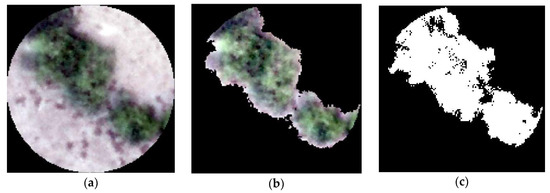
Figure 3.
The calculation diagram of VHOI: (a) The 7 cm multispectral image (representing the real scene in this paper); (b) Vegetation pixels in the multispectral image, and representative the vegetation of real scene; (c) representing the 7 cm binary raster image obtained from binarization operation to TLS PCD (white for the vegetation). The edge length of (a–c) is all 10 m.
3.2.2. STLS Computed from TLS Data
To obtain horizontal projected area of TLS-based scene vegetation, we first converted the TLS data into binary raster images (Figure 3c) by horizontal projection, with 1 representing vegetation and 0 representing non-vegetation, and then counted the vegetation pixels in each plot.
where refers to the number of vegetation cells in the binary raster image; refers to the edge length of a cell in the binary raster image which we defined as 7 cm, the same as .
Therefore, the VHOI calculation can be simplified as Equation (4):
3.3. LAI Estimation
In this study, the LAI estimation is based on gap fraction theory, as shown in Equation (5)
where refers to the angle between the light incidence direction and the vertical direction, i.e., the zenith angle; refers to the canopy gap fraction at zenith angle ; and is the extinction coefficient, i.e., the average projected area of a unit leaf area in a plane perpendicular to the direction of the beam.
Different mathematical models for have been summarized [23]. In our experiment, the approximate ellipsoidal model for the extinction coefficient was utilized, as shown in the following equation
where is a shape parameter of the leaf angle distribution. In our study, leaf angle was assumed to follow a spherical distribution ( = 1) [2,14,23]. Namely, is constant (i.e., = 0.500) by calculation Equation (6). Combining Equations (5) and (6) with = 1, LAI was only determined by the canopy gap fraction at different zenith angle, as shown in Equation (7).
To calculate the gap fraction at different zenith angle, we used the mathematical theory which was given by Zheng [20]. The 3-D canopy-only PCD of each plot first was projected to two-dimensional (2-D) raster images like “hemispherical photograph” through the following steps: (1) The Cartesian coordinate system (X, Y, Z) of each plot were converted to the spherical coordinate system with a radius of 0.1 m. The X and Y values of the origin point were used to project all points onto the hemisphere surface, which was the X and Y of the centroid of the plot, while the Z value of the original was the Z of the lowest point of the 3-D canopy-only PCD. It should be noted that the radius value did not affect the results [20]. (2) The spherical coordinates of each plot were transformed into the 2-D plane through the stereographic projection. The 2-D plane of each plot, which was perpendicular to the Z direction was converted to raster images with resolution of 7 cm through the rasterization processes. Each pixel containing TLS points (i.e., foliage elements) was represented by 0 and non-vegetation pixels which did not contain points were represented by 1. Next, the Gap Light Analyzer (GLA) software (Spatial Solutions, Inc., Victoria, B.C. Canada) was used to analyze and process 2-D raster images. Each raster image was divided into nine annulus rings with an interval of 10° representing the zenith angle ranges. Finally, the canopy gap fraction at different zenith angle was computed using GLA software though calculating the ratio of the total area of non-vegetation pixel for the annulus ring to the total area of the annulus ring.
4. Results and Discussion
4.1. Relationship between VHOI and Estimation Accuracy
We calculated VHOI of the 102 plots using TLS PCD and UAV optical images in the dense mangrove forests. The regression analysis of VHOI against estimation accuracy was performed using a linear model (see Figure 4). The absolute percentage error (APE) is used to assess the estimation accuracy, which is defined as the absolute value of the ratio of the difference between the field-measured LAI and estimated LAI, with the range from 0 to 1. Lower APE means less deviation between the TLS-estimated LAI and the field-measured value, thus higher estimation accuracy. We used R2 and root mean squared error (RMSE) to assess the degree of fitness of the regression model. The strong relationship (R2 = 0.72, RMSE = 0.137) between VHOI and APE is shown in Figure 4. This result shows that VHOI can be used to indicate LAI estimation accuracy.
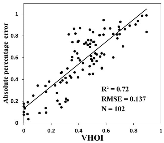
Figure 4.
The relationship between VHOI and absolute percentage error (APE).
As shown in Figure 4, VHOI values of four plots are 0. Actually, the four values are all negative and are replaced with 0. Some VHOI values lower than 0 were caused by the factor that some mangrove pixels were misclassified as non-mangrove (soil or water). The user accuracy and producer accuracy of mangrove class were 85.83% and 96.26%, respectively.
Although the resolution of commercial UAV multispectral images (7 cm) is fine enough, some factors still limit the classification accuracy, such as shaded background, the edge between different classes, and small crown gaps. This conclusion is in good agreement with those reported by Tian [7], who compared the ability for LAI mapping using UAV and WorldView-2 imagery in dense mangrove forests. Thus, some other UAV images with higher spatial resolution are needed to improve the classification accuracy.
In this paper, the calculation of VHOI needed to combine the TLS data and the high-resolution optical image. UAV platforms have opened the door to acquire high spatial-resolution optical image data because it is flexible in terms of flying height and viewing angles as compared to traditional satellite and airborne remote sensing platforms [36,37,38,39]. However, the commercial UAV platform is still not convenient to acquired data for large area mapping or multi-temporal analysis. Moreover, it is still expensive in terms of the on-demand acquisition [40]. This is a serious inhibition of the popularization of VHOI. The development of consumer UAV platforms will help promote the popularization of VHOI because it offers high-resolution at more flexible times and places and lower cost, in contrast with commercial UAV platforms.
Figure 4 shows that there is a large variation in APE with similar VHOI values, especially for VHOI between 0.4 and 0.7. That VHOI only represent the horizontal occlusion is the important factor causing the large deviation. In terms of VHOI calculation, TLS data need planarization. The planarization is the data process where the 3-D coordinates of the PCD are projected onto a horizontal plane with horizontal projection and then converted to binary raster images through a rasterization procedure (detailed processes see Section 3.2.2). It will make the vertical structure information of PCD loss and the horizontal structure information retention. This process thus easily results in the situation that the same value of VHOI and different LAI are derived from PCD with similar horizontal structure information and different vertical distribution pattern. Accurate representation occlusion needs the vertical structure information. Several previous studies have comprehensively described occlusion through the consideration of laser pulse trajectory [25,26,34]. Paynter [26] has used the above method to compute the regions of occlusion of a single tree and of a deciduous forest from TLS data. However, the 3-D profile of complete vegetation object cannot determine in terms of this model. Thus, the combination of high-resolution UAV datasets and the ray tracing method based on voxel may be a good methodological framework for quantitatively characterizing occlusion.
4.2. Estimation Accuracy of LAI with Different VHOI
In Section 4.1, we concluded that VHOI could be used to quantitatively represent data quality. The lower the value of VHOI is, the higher the data quality is. In order to find the threshold of VHOI to best separate high-quality data and poor-quality data, the relationship between LAI generated from TLS data that is selected with different ranges of VHOI and field-measured data is discussed. As shown in Figure 5, when the VHOI of the plots is less than or equal to a certain threshold (0.1, 0.2, 0.3, 0.4, 0.5, 0.6, 0.7, 0.8 and 0.9), the relationship (R2) approximately present a declining trend and the relative RMSE (%RMSE) has an opposite trend. %RMSE is expressed as a percentage between RMSE and the mean value of the field LAI [7,41]. It should be noted that none of the plots has VHOI value over 0.9. The increased amount of poor-quality data with the increase of the VHOI threshold is the main factor causing the above trends.
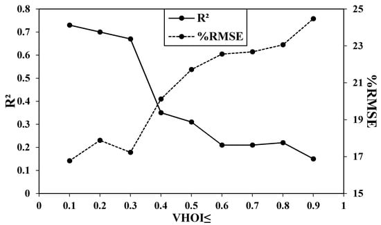
Figure 5.
Changes in R2 (solid line) and %RMSE (dotted line) with different value of VHOIs.
From Figure 5, we can observe that the accuracy of TLS-based LAI is similar among all plots whose VHOI values are between 0 and 0.3, as the R2 between TLS-based LAI and LAI2200-based LAI are similar (0.67–0.73). This is further confirmed from the scatterplots in Figure 6. From Figure 6b,c, when the ranges of VHOI value are 0–0.2 and 0–0.25, the relationship (R2) between LAI derived from TLS and LAI value measured from LAI2200 PCA and the number of plot (N) are 0.70 and 0.72, 16 and 19, respectively. This is slightly different from the expected decreasing trend. The main reason is that the three plots with VHOI value between 0.2 and 0.25 have relatively better LAI accuracy than the other plots. We consider this to be a normal variation as the TLS data has similar quality when VHOI is less than 0.30.
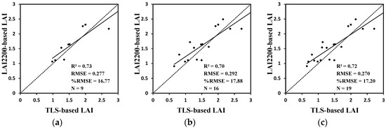
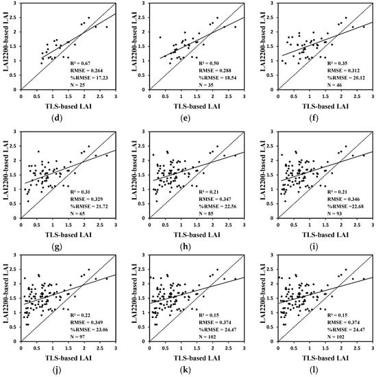
Figure 6.
The R2, RMSE, %RMSE between LAI estimated from TLS and LAI from LAI2200 PCA, and the number of plots (N) under the different threshold of VHOI. The range of VHOI is 0–0.1 (a), 0–0.2 (b), 0–0.25 (c), 0–0.3 (d), 0–0.35 (e), 0–0.4 (f), 0–0.5 (g), 0–0.6 (h), 0–0.7 (i), 0–0.8 (j), 0–0.9 (k), 0–1.0 (l), respectively. The dotted line is 1:1 line; solid line depicts regression fit.
As shown in Figure 6l, compared with field LAI, a total number of 97 estimation values derived from TLS data were underestimated. Meanwhile, the number of overestimated LAI value was only five. The loss of structure information caused by occlusion is the main reason why the number of underestimated plots was far greater than the overestimated ones.
As VHOI threshold changes from 0.3 to 0.35, R2 drops from 0.67 to 0.5 (see Figure 6d,e). When the threshold of VHOI is over 0.35, the maximum value of the R2 is only 0.5 (VHOI ≤ 0.35). However, for VHOI threshold below 0.3, the minimum value of the R2 can reach 0.67 (VHOI ≤ 0.3). This indicates that VHOI can be applied to select high-quality data. Furthermore, in this study, we can see that the maximum threshold of VHOI for distinguishing high-quality and poor-quality data is 0.3. In other words, we consider that the VHOI value of high-quality data is less than or equal to 0.3. The VHOI threshold of 0.3 is only the advisory threshold in terms of dense mangrove LAI retrieval at plot scale. This threshold, thus, may be inapplicable for LAI estimation in other types of forests. However, we believe that the method for selecting high-quality TLS data is suitable for other types of forests. In addition, we also consider that filtering TLS data by VHOI can improve the estimation accuracy of other structure parameters, such as canopy structure and biomass, because accurate estimation of these parameters heavily relied on high-quality data.
Instead of the true LAI, the effective LAI was estimated in the study. Different from calculating effective LAI, which assumes the leaves are randomly distributed in canopy and treats all plant parts as leaves, the calculation of the true LAI requires eliminating the effect of two factors: (1) foliage clumping and (2) non-photosynthetic tissues, such as trunks, branches [42]. To eliminate the effect of foliage clumping, the clumping index is introduced. Generally, if the crown canopy is randomly distributed, the value of the foliage clumping index is 1 [43]. However, in many cases, the distribution of leaves is non-random. Some studies [44,45,46], therefore, attached importance to developing methods to estimate the clumping index. Li [44] calculated the clumping index based on the theory of gap size distribution. This research showed the ability of the TLS technology to calculate the clumping index at the individual-tree level, but may not be applicable for mangrove forests at plot level because they are heterogeneous. Therefore, our future research includes developing new methods to calculate the clumping index of mangroves at the plot scale. Additionally, non-photosynthetic tissues have a great impact on the estimation accuracy of true LAI, except for foliage clumping. Therefore, we also need to separate the photosynthetic and non-photosynthetic tissues to accurately calculate true LAI. Compared with TLS technology, although the hyper-spectral imaging technology is unavailable for characterizing the 3-D structure information, has a huge potential to distinguish the photosynthetic and non-photosynthetic tissues. The combination of TLS and hyper-spectral imaging technology can provide a new data source for calculating true LAI. The registration of these two technologies is the key to successful application. Our next work, thus, will be dedicated to the registration.
Unlike the ground validation data acquired by an LAI-2200 Plant Canopy Analyzer with measurement method from bottom to top, the PCD is acquired from single side lateral scanning. Thus, the relationship between TLS-derived LAI and ground validation LAI data has deviation. The common solutions use ground validation data from destructive samples [13,44]. However, as a protected species, mangroves are prohibited from being cut down, making it difficult to obtain destructive samples in mangrove ecosystems. That is a limitation of the TLS technology on estimating LAI of mangrove ecosystems.
5. Conclusions
This research presents an exploration of the ability of VHOI based on TLS dataset and high-resolution UAV image to quantitatively represent data quality and screen out the poor-quality data in terms of plot-level LAI retrieval. By analyzing the relationship of VHOI and estimation accuracy of TLS-derived LAI (R2 = 0.72, RMSE = 0.137), the study demonstrated that VHOI can quantitatively characterize TLS data quality. Then, a comparison of field-measured LAI and mangrove LAI exploited from TLS data that was selected by different VHOI thresholds (0.1–0.9) was conducted, the R2 had a decreasing trend, with a drastic change from 0.67 to 0.50 when the threshold increased from 0.3 to 0.35, respectively. The results showed that the maximum critical threshold of VHOI for selecting high-quality data was 0.3 in our study. In summary, our study revealed that VHOI has the potential for improving estimation accuracy of dense mangrove LAI. Furthermore, we also concluded that TLS was an effective tool to yield dense mangrove LAI as long as high-quality data were acquired. Thus, we suggest that we should use VHOI to choose high-quality data before estimating the “shrub-type” mangrove LAI. It is obvious that it can be applied not only to pick out mangrove PCD for accurately estimating LAI, but also to choose other forest PCD for the retrieval of other structural parameters, such as biomass.
Author Contributions
X.G. designed, collected data, implemented the manual measurements and drafted the initial manuscript; L.W., J.T. and D.Y. supervised the analysis, and provided guidance on structure of manuscript. All authors read the manuscript, contributed to the discussion, and gave valuable suggestions to improve the manuscript.
Funding
This study was supported by “Capacity Building for Sci-Tech Innovation—Fundamental Scientific Research Funds (025185305000/199; 025185305000/211)” and “National Natural Science Foundation of China (41828102; 41801331; 41601363)”.
Acknowledgments
We are grateful to Yang Yu, Xinghe liu and Qianqian Wen for their assistance on data collection. In addition, we appreciate Drs: Jin Chen, Qinghua Guo and Yong Pang for constructive comments on the manuscript. We also thank the anonymous reviewers for helpful insights in improving this paper.
Conflicts of Interest
The authors declare no conflict of interest.
References
- Chen, J.M.; Black, T. Defining leaf area index for non-flat leaves. Plant Cell Environ. 1992, 15, 421–429. [Google Scholar] [CrossRef]
- Zheng, G.; Moskal, L.M. Retrieving leaf area index (LAI) using remote sensing: Theories, methods and sensors. Sensors 2009, 9, 2719–2745. [Google Scholar] [CrossRef] [PubMed]
- Tian, J.; Wang, L.; Li, X.; Shi, C.; Gong, H. Differentiating tree and shrub lai in a mixed forest with icesat/glas spaceborne LiDAR. IEEE J. Sel. Top. Appl. Earth Observ. Remote Sens. 2017, 10, 87–94. [Google Scholar] [CrossRef]
- Kamal, M.; Phinn, S.; Johansen, K. Assessment of multi-resolution image data for mangrove leaf area index mapping. Remote Sens. Environ. 2016, 176, 242–254. [Google Scholar] [CrossRef]
- Jensen, J.R.; Lin, H.; Yang, X.; Ramsey, E., III; Davis, B.A.; Thoemke, C.W. The measurement of mangrove characteristics in southwest Florida using spot multispectral data. Geocarto Int. 1991, 6, 13–21. [Google Scholar] [CrossRef]
- Heumann, B.W. Satellite remote sensing of mangrove forests: Recent advances and future opportunities. Progr. Phys. Geogr. 2011, 35, 87–108. [Google Scholar] [CrossRef]
- Tian, J.; Wang, L.; Li, X.; Gong, H.; Shi, C.; Zhong, R.; Liu, X. Comparison of UAV and worldview-2 imagery for mapping leaf area index of mangrove forest. Int. J. Appl. Earth Obs. Geoinf. 2017, 61, 22–31. [Google Scholar] [CrossRef]
- Green, E.P.; Mumby, P.J.; Edwards, A.J.; Clark, C.D.; Ellis, A.C. Estimating leaf area index of mangroves from satellite data. Aquat. Bot. 1997, 58, 11–19. [Google Scholar] [CrossRef]
- Van der Zande, D.; Hoet, W.; Jonckheere, I.; van Aardt, J.; Coppin, P. Influence of measurement set-up of ground-based LiDAR for derivation of tree structure. Agric. For. Meteorol. 2006, 141, 147–160. [Google Scholar] [CrossRef]
- Greaves, H.E.; Vierling, L.A.; Eitel, J.U.H.; Boelman, N.T.; Magney, T.S.; Prager, C.M.; Griffin, K.L. Estimating aboveground biomass and leaf area of low-stature Arctic shrubs with terrestrial LiDAR. Remote Sens. Environ. 2015, 164, 26–35. [Google Scholar] [CrossRef]
- Jonckheere, I.; Fleck, S.; Nackaerts, K.; Muys, B.; Coppin, P.; Weiss, M.; Baret, F. Review of methods for in situ leaf area index determination: Part I. Theories, sensors and hemispherical photography. Agric. For. Meteorol. 2004, 121, 19–35. [Google Scholar] [CrossRef]
- Breda, N.J. Ground-based measurements of leaf area index: A review of methods, instruments and current controversies. J. Exp. Bot. 2003, 54, 2403–2417. [Google Scholar] [CrossRef] [PubMed]
- Olsoy, P.J.; Mitchell, J.J.; Levia, D.F.; Clark, P.E.; Glenn, N.F. Estimation of big sagebrush leaf area index with terrestrial laser scanning. Ecol. Indic. 2016, 61, 815–821. [Google Scholar] [CrossRef]
- Zhao, F.; Yang, X.; Schull, M.A.; Román-Colón, M.O.; Yao, T.; Wang, Z.; Zhang, Q.; Jupp, D.L.B.; Lovell, J.L.; Culvenor, D.S.; et al. Measuring effective leaf area index, foliage profile, and stand height in New England forest stands using a full-waveform ground-based LiDAR. Remote Sens. Environ. 2011, 115, 2954–2964. [Google Scholar] [CrossRef]
- Yun, T.; Li, W.; Sun, Y.; Xue, L. Study of subtropical forestry index retrieval using terrestrial laser scanning and hemispherical photography. Math. Probl. Eng. 2015, 2015, 206108. [Google Scholar] [CrossRef]
- Danson, F.M.; Hetherington, D.; Morsdorf, F.; Koetz, B.; Allgower, B. Forest canopy gap fraction from terrestrial laser scanning. IEEE Geosci. Remote Sens. Lett. 2007, 4, 157–160. [Google Scholar] [CrossRef]
- Hopkinson, C.; Lovell, J.; Chasmer, L.; Jupp, D.; Kljun, N.; van Gorsel, E. Integrating terrestrial and airborne LiDAR to calibrate a 3D canopy model of effective leaf area index. Remote Sens. Environ. 2013, 136, 301–314. [Google Scholar] [CrossRef]
- Nie, S.; Wang, C.; Dong, P.; Xi, X. Estimating leaf area index of maize using airborne full-waveform LiDAR data. Remote Sens. Lett. 2015, 7, 111–120. [Google Scholar] [CrossRef]
- Pueschel, P.; Newnham, G.; Hill, J. Retrieval of gap fraction and effective plant area index from phase-shift terrestrial laser scans. Remote Sens. 2014, 6, 2601–2627. [Google Scholar] [CrossRef]
- Zheng, G.; Moskal, L.M.; Kim, S.-H. Retrieval of effective leaf area index in heterogeneous forests with terrestrial laser scanning. IEEE Trans. Geosci. Remote Sens. 2013, 51, 777–786. [Google Scholar] [CrossRef]
- Jupp, D.L.; Culvenor, D.; Lovell, J.; Newnham, G.; Strahler, A.; Woodcock, C. Estimating forest LAI profiles and structural parameters using a ground-based laser called ‘echidna®. Tree Physiol. 2009, 29, 171–181. [Google Scholar] [CrossRef] [PubMed]
- Zheng, G.; Moskal, L.M. Computational-geometry-based retrieval of effective leaf area index using terrestrial laser scanning. IEEE Trans. Geosci. Remote Sens. 2012, 50, 3958–3969. [Google Scholar] [CrossRef]
- Zhao, K.; García, M.; Liu, S.; Guo, Q.; Chen, G.; Zhang, X.; Zhou, Y.; Meng, X. Terrestrial LiDAR remote sensing of forests: Maximum likelihood estimates of canopy profile, leaf area index, and leaf angle distribution. Agric. For. Meteorol. 2015, 209, 100–113. [Google Scholar] [CrossRef]
- Li, A.; Glenn, N.F.; Olsoy, P.J.; Mitchell, J.J.; Shresth, R. Aboveground biomass estimates of sagebrush using terrestrial and airborne LiDAR data in a dryland ecosystem. Agric. For. Meteorol. 2015, 213, 138–147. [Google Scholar] [CrossRef]
- Kükenbrink, D.; Schneider, F.D.; Leiterer, R.; Schaepman, M.E.; Morsdorf, F. Quantification of hidden canopy volume of airborne laser scanning data using a voxel traversal algorithm. Remote Sens. Environ. 2017, 194, 424–436. [Google Scholar] [CrossRef]
- Paynter, I.; Genest, D.; Saenz, E.; Peri, F.; Li, Z.; Strahler, A.; Schaaf, C. Quality Assessment of Terrestrial Laser Scanner Ecosystem Observations Using Pulse Trajectories. IEEE Trans. Geosci. Remote Sens. 2018, 56, 6324–6333. [Google Scholar]
- Yang, S.; Wang, L.; Shi, C.; Lu, Y. Evaluating the relationship between the photochemical reflectance index and light use efficiency in a mangrove forest with spartina alterniflora invasion. Int. J. Appl. Earth Obs. Geoinf. 2018, 73, 778–785. [Google Scholar] [CrossRef]
- Wang, L.; Shi, C.; Tian, J.; Song, X.; Jia, M.; Li, X.; Liu, X.; Zhong, R.; Yin, D.; Yang, S.; et al. Researches on mangrove forest monitoring methods based on multi-source remote sensing. Biodivers. Sci. 2018, 26, 838–849. [Google Scholar]
- Wang, L.; Silvan, J.; Sousa, W. Neural network classification of mangrove species from multiseasonal IKONOS imagery. Photogramm. Eng. Remote Sens. 2008, 74, 921–927. [Google Scholar] [CrossRef]
- Wang, L.; Sousa, W.P.; Gong, P.; Biging, G.S. Comparison of IKONOS and QuickBird images for mapping mangrove species on the Caribbean coast of Panama. Remote Sens. Environ. 2004, 91, 432–440. [Google Scholar] [CrossRef]
- Wang, L.; Sousa, W.; Gong, P. Integration of object-based and pixel-based classification for mapping mangroves with IKONOS imagery. Int. J. Remote Sens. 2004, 25, 5655–5668. [Google Scholar] [CrossRef]
- Feliciano, E.A.; Wdowinski, S.; Potts, M.D. Assessing mangrove above-ground biomass and structure using terrestrial laser scanning: A case study in the Everglades National Park. Wetlands 2014, 34, 955–968. [Google Scholar] [CrossRef]
- Zheng, G.; Moskal, L.M. Spatial variability of terrestrial laser scanning based leaf area index. Int. J. Appl. Earth Obs. Geoinf. 2012, 19, 226–237. [Google Scholar] [CrossRef]
- Béland, M.; Widlowski, J.-L.; Fournier, R.A.; Côté, J.-F.; Verstraete, M.M. Estimating leaf area distribution in savanna trees from terrestrial LiDAR measurements. Agric. For. Meteorol. 2011, 151, 1252–1266. [Google Scholar] [CrossRef]
- Hosoi, F.; Omasa, K. Voxel-based 3-D modeling of individual trees for estimating leaf area density using high-resolution portable scanning LiDAR. IEEE Trans. Geosci. Remote Sens 2006, 44, 3610–3618. [Google Scholar] [CrossRef]
- Tian, J.; Wang, L.; Li, X. Sub-footprint analysis to uncover tree height variation using ICESat/GLAS. Int. J. Appl. Earth Obs. Geoinf. 2015, 35, 284–293. [Google Scholar] [CrossRef]
- Turner, D.; Lucieer, A.; Malenovský, Z.; King, D.H.; Robinson, S.A. Spatial co-registration of ultra-high resolution visible, multispectral and thermal images acquired with a micro-UAV over antarctic moss beds. Remote Sens. 2014, 6, 4003–4024. [Google Scholar] [CrossRef]
- Knoth, C.; Klein, B.; Prinz, T.; Kleinebecker, T. Unmanned aerial vehicles as innovative remote sensing platforms for high-resolution infrared imagery to support restoration monitoring in cut-over bogs. Appl. Veg. Sci. 2013, 16, 509–517. [Google Scholar] [CrossRef]
- Tian, J.; Li, X.; Duan, F.; Wang, J.; Ou, Y. An efficient seam elimination method for uav images based on wallis dodging and gaussian distance weight enhancement. Sensors 2016, 16, 662. [Google Scholar] [CrossRef] [PubMed]
- Liu, X.; Wang, L. Feasibility of using consumer-grade unmanned aerial vehicles to estimate leaf area index in mangrove forest. Remote Sens. Lett. 2018, 9, 1040–1049. [Google Scholar] [CrossRef]
- Yin, D.; Wang, L. How to assess the accuracy of the individual tree-based forest inventory derived from remotely sensed data: A review. Int. J. Remote Sens. 2016, 37, 4521–4553. [Google Scholar] [CrossRef]
- Weiss, M.; Baret, F.; Smith, G.; Jonckheere, I.; Coppin, P. Review of methods for in situ leaf area index (LAI) determination: Part II. Estimation of LAI, errors and sampling. Agric. For. Meteorol. 2004, 121, 37–53. [Google Scholar] [CrossRef]
- Chen, J.; Black, T.; Adams, R. Evaluation of hemispherical photography for determining plant area index and geometry of a forest stand. Agric. For. Meteorol. 1991, 56, 129–143. [Google Scholar] [CrossRef]
- Li, Y.; Guo, Q.; Su, Y.; Tao, S.; Zhao, K.; Xu, G. Retrieving the gap fraction, element clumping index, and leaf area index of individual trees using single-scan data from a terrestrial laser scanner. ISPRS J. Photogramm. 2017, 130, 308–316. [Google Scholar] [CrossRef]
- Zhao, F.; Strahler, A.H.; Schaaf, C.L.; Yao, T.; Yang, X.; Wang, Z.; Schull, M.A.; Román, M.O.; Woodcock, C.E.; Olofsson, P. Measuring gap fraction, element clumping index and LAI in Sierra Forest stands using a full-waveform ground-based lidar. Remote Sens. Environ. 2012, 125, 73–79. [Google Scholar] [CrossRef]
- Bailey, B.N.; Mahaffee, W.F. Rapid measurement of the three-dimensional distribution of leaf orientation and the leaf angle probability density function using terrestrial LiDAR scanning. Remote Sens. Environ. 2017, 194, 63–76. [Google Scholar] [CrossRef]
© 2018 by the authors. Licensee MDPI, Basel, Switzerland. This article is an open access article distributed under the terms and conditions of the Creative Commons Attribution (CC BY) license (http://creativecommons.org/licenses/by/4.0/).